Báo cáo hóa học: " Research Article New Technique for Improving Performance of LDPC Codes in the Presence of Trapping S" doc

Hindawi Publishing Corporation
EURASIP Journal on Wireless Communications and Networking
Volume 2008, Article ID 362897, 12 pages
doi:10.1155/2008/362897
Research Article
New Technique for Improving Performance of LDPC Codes in
the Presence of Trapping Sets
Esa Alghonaim,
1
Aiman El-Maleh,
1
and Mohamed Adnan Landolsi
2
1
Computer Engineering Department, King Fahd University of Petroleum & Minerals, Dhahran 31261, Kingdom of Saudi Arabia
2
Electrical Engineering Depart ment, King Fahd University of Petroleum & Minerals, Dhahran 31261, Kingdom of Saudi Arabia
Correspondence should be addressed to Esa Alghonaim,
Received 2 December 2007; Revised 18 February 2008; Accepted 21 April 2008
Recommended by Yonghui Li
Trapping sets are considered the primary factor for degrading the performance of low-density parity-check (LDPC) codes in the
error-floor region. The effect of trapping sets on the performance of an LDPC code becomes worse as the code size decreases.
One approach to tackle this problem is to minimize trapping sets during LDPC code design. However, while trapping sets can
be reduced, their complete elimination is infeasible due to the presence of cycles in the underlying LDPC code bipartite graph.
In this work, we introduce a new technique based on trapping sets neutralization to minimize the negative effect of trapping sets
under belief propagation (BP) decoding. Simulation results for random, progressive edge growth (PEG) and MacKay LDPC codes
demonstrate the effectiveness of the proposed technique. The hardware cost of the proposed technique is also shown to be minimal.
Copyright © 2008 Esa Alghonaim et al. This is an open access article distributed under the Creative Commons Attribution License,
which permits unrestricted use, distribution, and reproduction in any medium, provided the original work is properly cited.
1. INTRODUCTION
Forward error correcting (FEC) codes are an essential com-

ponent of modern state-of-the-art digital communication
and storage systems. Indeed, in many of the recently devel-
oped standards, FEC codes play a crucial role for improving
the error performance capability of digital transmission over
noisy and interference-impaired communication channels.
Low-density parity-check codes (LDPCs), originally
introduced in [1], have recently been undergoing a lot
of active research and are now widely considered to be
one of the leading families of FEC codes. LDPC codes
demonstrate performance very close to the information-
theoretic bounds predicted by Shannon theory, while at the
same time having the distinct advantage of low-complexity,
near-optimal iterative decoding.
As with other types of codes decoded by iterative decod-
ing algorithms (such as turbo codes), LDPC codes can suffer
from the presence of undesirable error floors at increasing
SNR levels (although these are found to be relatively lower
than the error floors encountered with turbo codes [2]).
In the case of LDPC codes, trapping sets [2–4]havebeen
identified as one of the main factors causing error floors
at high SNR values. The analysis of trapping sets and their
impact on LDPC codes has been addressed in [3, 5–9]. The
main approaches for mitigating the impact of trapping sets
on LDPC codes are based on either introducing algorithms
to minimize their presence during code design as in [5, 7, 9]
or by enhancing decoder performance in the presence of
trapping sets as in [3, 6, 8]. The main disadvantage of the
first approach, in addition to putting tight constraints on
code design, is that trapping sets cannot be totally eliminated
at the end due to the “unavoidable” existence of cycles

in their underlying bipartite Tanner graphs especially for
relatively short block length codes (which is the focus of this
work). In addition, LDPC codes designed to reduce trapping
sets may result in large interconnect complexity increasing
hardware implementation overhead. The second approach is
therefore considered to be more applicable for our purpose
and is the basis of the contributions presented in this
paper.
In order to enhance decoder performance in the presence
of (unavoidable) trapping sets, an algorithm is introduced
in [3] based on flipping the hard decoded bits in trapping
sets. First, trapping sets are identified and stored in a
lookup table based on BP decoding simulation. Whenever
the decoder fails, the decoder uses the lookup table based
on the unsatisfied parity checks to determine if a preknown
failure is detected. If a match occurs, the decoder simply
flips the hard decision values of trapping bits. This approach
2 EURASIP Journal on Wireless Communications and Networking
suffers from the following disadvantages: (1) the decoder has
to exactly specify the trapping sets variable nodes in order
to flip them; (2) extra time is needed to search the lookup
table for a trapping set; (3) the technique is not amenable to
practical hardware implementation.
In [6, 8], the concept of averaging partial results is used to
overcome the negative effect of trapping sets in the error floor
region. Variable node messages update in the conventional
BP decoder are modified in order to make it less sensitive
to oscillations in messages received from check nodes. The
variable node equation is modified to be the average of
current and previous signals values received from check

nodes. While this approach is effective in handling oscillating
error patterns, it does not improve decoder performance in
the case of constant error patterns.
In this paper, we propose a novel approach for enhanc-
ing decoder performance in presence of trapping sets by
introducing a new concept called trapping sets neutralization.
The effect of a trapping set can be eliminated by setting its
variable nodes intrinsic and extrinsic values to zero, that
is, neutralizing them. After a trapping set is neutralized,
the estimated values of variable nodes are affected only by
external messages from nodes outside the trapping set.
Most harmful trapping sets are identified by means of
simulation. To be able to neutralize identified trapping sets,
a simple algorithm is introduced to store trapping sets
configuration information in variable and check nodes.
The remainder of this paper is organized as follows:
In Section 2,wegiveanoverviewofLDPCcodesandBP
algorithm. Trapping sets identification and neutralization are
introduced in Section 3. Section 4 presents the algorithm of
trapping sets neutralization based on learning. Experimental
results are given in Section 5.InSection 6, we conclude the
paper.
2. OVERVIEW OF LDPC CODES
LDPC codes are a class of linear block codes that use a sparse,
random-like parity-check matrix H [1, 10]. An LDPC code
defined by the parity-check matrix H represents the parity
equations in a linear form, where any given codeword u
satisfies the set of parity equations such that u
×H = 0.Each
column in the matrix represents a codeword bit while each

row represents a parity-check equation.
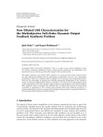
LDPC codes can also be represented by bipartite graphs,
usually called Tanner graphs, having two types of nodes:
variable nodes and check nodes interconnected by edges
whenever a given information bit appears in the parity-
check equation of the corresponding check bit, as shown in
Figure 1.
The properties for an (N, K) LDPC code specified by an
M
×N H matrix can be summarized as follows.
– Block size: number of columns (N) in the H matrix.
– Number of information bits: given by K
= N −M.
– Rate: the rate of the information bits to the block
size. It equals 1
−M/N, given that there are no linear
dependent rows in the H matrix.
v
1
v
2
v
3
v
4
v
5
c
1
c

2
c
3
v
1
v
2
v
3
v
4
v
5
c
1
c
2
c
3
+
+
+
H
=
⎡
⎢
⎣
11110
10101
01011

⎤
⎥
⎦
Figure 1: The two representations of LDPC codes: graph form and
matrix form.
– Check node degree: number of 1’s in the correspond-
ing row in the H matrix. Degree of a check node c
j
is
referred to as d(c
j
).
– Variable node degree: number of 1’s in the corre-
sponding column in the H matrix. Degree of a
variable node v
i
is referred to as d(v
i
).
– Regularity: an LDPC code is said to be regular if
d(v
i
) = p for 1 ≤ i ≤ N and d(c
j
) = q for 1 ≤ j ≤ M.
In this case, the code is (p, q) regular LDPC code.
Otherwise, the code is considered irregular.
– Code girth: the minimum cycle length in the Tanner
graph of the code.
The iterative message-passing belief propagation algorithm

(BP) [1, 10] is commonly used for decoding LDPC codes
and is shown to achieve optimum performance when the
underlying code graph is cycle-free. In the following, a
brief summary of the BP algorithm is given. Following
the notation and terminology used in [11], we define the
following:
(i) u
i
: transmitted bit in a codeword, u
i
∈{0,1}.
(ii) x
i
: a transmitted channel symbol, with a value given
by
x
i
=
⎧
⎨
⎩
+1, when u
i
= 0
−1, when u
i
= 1.
(1)
(iii) y
i

: a received channel symbol, y
i
= x
i
+ n
i
,wheren
i
is zero-mean additive white Gaussian noise (AWGN)
random variable with variance σ
2
.
(iv) For the jth row in an H matrix, the set of column
locationshaving1’sisgivenbyR
j
={i : h
ji
= 1}.The
set of column locations having 1’s, excluding location
I,isgivenbyR
j\i
={i

: h
ji

= 1}\{i}.
(v) For the ith column in an H matrix, the set of row
locationshaving1’sisgivenbyC
i

={j : h
ji
= 1}.The
set of row locations having 1’s, excluding the location
j,isgivenbyC
i\j
={j

: h
j

i
= 1}\{j}.
Esa Alghonaim et al. 3
c
j
q
ij
(b)
v
i
(a)
c
j
r
ji
(b)
v
i
(b)

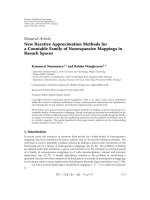
Figure 2: (a) Variable-to-check message, (b) check-to-variable
message.
(vi) q
ij
(b): message (extrinsic information) to be passed
from variable node v
i
to check node c
j
regarding
the probability of u
i
= b, b ∈{0, 1}, as shown in
Figure 2(a). It equals the probability that u
i
= b given
extrinsic information from all check nodes, except
node c
j
.
(vii) r
ji
(b): message to be passed from check node c
j
to
variable node v
i
, which is the probability that the jth
check equation is satisfied given that bit u
i

= b and
the other bits have separable (independent) distribu-
tion given by
{q
ij

}
j

/
= j
, as shown in Figure 2(b).
(viii) Q
i
(b) = the probability that u
i
= b, b ∈{0,1}.
(ix)
L(u
i
) ≡ log
Pr(x
i
= +1 | y
i
)
Pr(x
i
=−1 | y
i

)
= log
Pr(u
i
= 0 | y
i
)
Pr(u
i
= 1 | y
i
)
,
(2)
where L(u
i
) is usually referred to as the intrinsic
information for node v
i
.
(x)
L(r
ji
) ≡ log
r
ji
(0)
r
ji
(1)

, L(q
ij
) ≡ log
q
ij
(0)
q
ij
(1)
. (3)
(xi)
L(Q
i
) ≡ log
Q
i
(0)
Q
i
(1)
. (4)
The BP algorithm involves one initialization step and three
iterative steps as shown below.
Initialization step
Set the initial value of each variable node signal as follows:
L(q
ij
) ≡ L(u
i
) = 2y

i
/σ
2
,whereσ
2
is the variance of noise in
the AWGN channel.
Iterative steps
The three iterative steps are as follows.
(i) Update check nodes as follows:
L

r
ji

=


i

∈R
j\i
α
i

j

×
φ



i

∈R
j\i
φ

β
i

j


,(5)
where α
i

j
= sign(L(q
ij
)), β
ij
=|L(q
ij
)|,
φ(x)
=−log

tanh(x/2)


=
log
e
x
+1
e
x
−1
. (6)
(ii) Update variable nodes as follows:
L(q
ij
) = L(u
i
)+

j

∈C
i\j
L

r
j

i

. (7)
(iii) Compute estimated variable nodes as follows:
L(Q

i
) = L

u
i

+

j∈C
i
L

r
ji

. (8)
Based on L(Q
i
), the estimated value of the received bit (u
i
)is
given by
u
i
=
⎧
⎨
⎩
1, if L


Q
i

< 0,
0, else.
(9)
During LDPC decoding, the iterative steps (i) to (iii) are
repeated until one of the following two events occurs:
(i) the estimated vector
u = (u
1
, , u
n
) satisfies the
check equations, that is,
u ·H = 0;
(ii) maximum iterations number is reached.
3. TRAPPING SETS
In BP decoding of LDPC codes, dominant decoding failures
are, in general, caused by a combination of multiple cycles
[4]. In [2], the combination of error bits that leads to a
decoder failure is defined as trapping sets. In [3], it is shown
that the dominant trapping sets are formed by a combination
of short cycles present in the bipartite graph.
In the following, we adopt the terminology and notation
related to trapping sets as originally introduced in [8]. Let
H be the parity-check matrix of (N, K)LDPCcode,andlet
G(H) denote its corresponding Tanner graph.
Definition 1. A(z, w) trapping set T is a set of z variable
nodes, for which the subgraph of the z variable nodes and

the check nodes that are directly connected to them contains
exactly w odd-degree check nodes.
The next example illustrates the behavior of trapping sets
and how they are harmful.
Example 2. Consider a regular (N, K) LDPC code with
degree (3,6). Figure 3 shows a trapping set T(4, 2) in the code
graph. Assume that an all-zero codeword (u
= 0) is sent
through an AWGN channel, and all bits are received correctly
(i.e., have positive intrinsic values) except the 4 bits in the
trapping set T(4, 2), that is, L(u
i
) < 0for1 ≤ i ≤ 4and
L(u
i
) > 0for4<i≤ N.(Assumelogic0isencodedas+1,
while logic 1 is encoded as
−1).
4 EURASIP Journal on Wireless Communications and Networking
v
1
v
2
v
3
v
4
c
1
c

2
c
3
c
4
c
5
c
6
c
7
Figure 3: Trapping set example of T(4, 2).
Based on (8), the estimated value of a variable node is the
sum of its intrinsic information and messages received from
the neighboring three check nodes. Therefore, the estimation
equation for each variable node contains four summation
terms: the intrinsic information and three information
messages. In this case, the estimated values for v
1
(and v
3
)
will be incorrect because all of the four summation terms
of its estimation equation are negative. For v
2
(and v
4
),
three out of the four summation terms in its estimation
equation have negative values. Therefore, v

2
(and v
4
)has
high probability to be incorrectly estimated. In this case,
the decoder becomes in trap and will continue in the trap
unless positive signals from c
1
and/or c
2
are strong enough
to change the polarities of the estimated values of v
2
and/or
v
4
. This example illustrates a trapping set causing a constant
error pattern.
As a first step to investigate the effect of trapping sets on
LDPC codes performance, extensive simulations for LDPC
codes over AWGN channels with various SNR values have
been performed. A frame is considered to be in error if the
maximum decoding iteration is reached without satisfying
the check equations, that is, the syndrome
u × H is nonzero.
Error frames are classified based on observing the behavior of
the LDPC decoder at each decoding iteration. At the end of
each iteration, bits in error are counted. Based on this, error
frames are classified into three patterns described as follows.
(i) Constant error pattern: where the bit error count

becomes constant after only a few decoding itera-
tions.
(ii) Oscillating error pattern: where the bit error count
follows a nearly periodic change between maximum
and minimum values. An important feature of this
error pattern is the high variation in bit error count
as a function of decoding iteration number.
(iii) Random-like error pattern: where the bit error count
evolution follows a random shape, characterized by
low variation range.
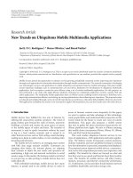
Figure 4 shows one example for each of the three error pat-
terns. In a constant error pattern, bit errors count becomes
constant after several decoding iterations (10 iterations in the
300
250
200
150
100
50
0
Number of error bits
0 10 20 30 40 50 60 70 80 90 100
Iteration
Oscillating
Constant
Random-like
Figure 4: Illustration of the three types of error patterns.
Table 1: Percentages of error patterns at error-floor region.
Code Size Constant Oscillating Random-like
HE(1024,512) 59% 38% 3%

RND(1024,512) 95% 4% 1%
PEG(100,50) 90% 5% 5%
example of Figure 4). In this case, the decoder becomes stuck
due to the presence of a tapping set T(z, w), and the number
of bits in error equals z and all check nodes are satisfied
except w check nodes.
The major difference between a trapping set T(z, w)
causing a constant error pattern and a trapping set T(e, f )
causing other patterns is the number of odd-degree check
nodes. Based on extensive simulations, it is found that w
≤
f . This result is interpreted logically as follows: if variable
nodes of a trapping set are in error, only odd-degree check
nodes are sending correct messages to the variable nodes of
the trapping set. Therefore, as the number of odd-degree
check nodes decreases, the probability of breaking the trap
decreases. As an extreme example, a trapping set with no
odd-degree check nodes results in a decoder convergence to
a codeword other than the transmitted one and thus causes
undetected decoder failure.
Ta ble 1 shows examples of percentages of the three error
patterns for three LDPC codes based on simulating the codes
at error-floor regions. The first LDPC code, HE(1024,512)
[12], is constructed to be interconnected efficiently for
fully parallel hardware implementation. The RND(1024,512)
LDPC code is randomly constructed avoiding cycles of size
4. The PEG(100,50) LDPC code is constructed using PEG
algorithm [7], which maximizes the size of cycles in the code
graph. From Ta bl e 1 , it is evident that constant error patterns
are significant in some LDPC codes including short length

codes.
Esa Alghonaim et al. 5
This observation motivates the need for developing
a technique for enhancing decoder performance due to
trapping sets of constant error patterns type. For trapping
sets that cause constant error patterns, when a trap occurs,
values of check equations do not change in subsequent
iterations. Thus, a decoder trap is detected based on check
equations results. The unsatisfied check nodes are used to
reach the trapping set variable nodes.
3.1. BP decoder trapping sets detec tion
In order to eliminate the effect of trapping sets during
the iterations of BP decoder, a mechanism is needed to
detect the presence of a trapping set. The proposed trapping
sets detection technique is based on monitoring the state
of the check equations vector
u × H. At the end of each
decoding iteration, a new value of
u × H is computed.
If the
u × H value is nonzero and remains unchanged
(stable) for a predetermined number of iterations, then a
decoder trap is detected. We call this number the stability
parameter (d), and it is normally set to a small value. Based
on experimental results, it is found that d
= 3 is a good
choice. The implementation of trap detection is similar to the
implementation of valid codeword detection with some extra
logic in each check node. Figure 5 shows an implementation
of trapping sets detection for a decoder with M check nodes.

The output s
i
for a check node c
i
is logic zero if the check
equation result is equivalent to the check equation result
in the previous iteration, that is, no change in the check
equation result. The output S is zero if there is no change
in all check equations between the current and the previous
iteration numbers.
3.2. Trapping sets neutralization
In this section, we introduce a new technique to overcome
the detrimental effect of trapping sets during BP decoding.
To overcome the negative impact of a trapping set T(z, w),
the basic idea is to neutralize the z variable nodes in the
trapping set. Neutralizing a variable node involves setting
its intrinsic value and extrinsic message values to zero.
Specifically, neutralizing a variable node v
i
involves the
following two steps:
(1) L(u
i
) = 0,
(2) L(q
ij
) = 0, 1 ≤ j ≤ d(v
i
).
The neutralization concept is illustrated by the following

example.
Example 3. For the trapping set T(4, 2) in Example 2,ithas
been shown that when all code bits are received correctly
except T(4, 2) bits, the decoder fails to correct the codeword
resulting in an error pattern of constant type.
Now, consider neutralizing the trapping set variable
nodes by setting its intrinsic and extrinsic values to zero.After
neutralization, the decoder converges to a valid codeword
within two iterations, as follows. In the first iteration after
neutralization, for v
2
and v
4
, two extrinsic messages become
positive due to positive messages from nodes c
1
and c
2
,
which shifts estimated values of v
2
and v
4
to the positive
correct values. For nodes v
1
and v
3
, all extrinsic values are
zeros and their estimated values remain zero. In the second

iteration after neutralization, for v
1
and v
3
, two extrinsic
messages become positive due to positive extrinsic messages
from nodes v
2
and v
4
, which shifts estimated values of v
1
and
v
3
to the positive correct values.
The proposed neutralization technique has three impor-
tant characteristics. (1) It is not necessary to exactly deter-
mine the variable nodes in a trapping set, such as the
trapping set bits flipping technique used in [3]. In the
previous example, if only 3 out of the 4 trapping sets variables
are neutralized, the decoder will still be able to recover
from the trap. (2) If some nodes outside a trapping set are
neutralized (due to inexact identification of the trapping set),
their extrinsic messages are expected to quickly recover their
estimation function to correct values due to correct messages
from neighbouring nodes. This is because most of the
extrinsic messages are correct in the error-floor regions. (3)
Neutralization is performed during BP decoding iterations as
soon as a trapping set is detected, which makes the decoder

able to converge to a valid codeword within the allowed
maximum number of iterations.
As an example, for the near-constant error pattern in
Figure 4, a trap occurs at iteration 10 and is detected at
iteration 13 (assuming d
= 3). In this case, the decoder
has a plenty of time to neutralize the trapping set before
reaching the maximum 100 iterations. In general, based on
our simulations, a decoder trap is detected during early
decoding iterations.
4. BP DECODER WITH TRAPPING SETS
NEUTRALIZATION BASED ON LEARNING
In this section, we introduce an algorithm to correct constant
error pattern types (causing error floors) associated with
LDPC BP decoding. The proposed algorithm involves two
parts: (1) a preprocessing phase called learning phase and
(2) actual decoding phase. The learning phase is an offline
computation process in which trapping sets are identified.
Then, variable and check nodes are configured according to
the identified trapping sets. In the actual decoding phase, the
proposed decoder runs as a standard BP decoder with the
ability to detect and neutralize trapping sets using variable
and check nodes configuration information obtained during
the learning phase. When a trapping set is detected, the
decoder stops running BP iterations and switches to a
neutralization process, in which the detected trapping set is
neutralized. Upon completion of the neutralization process,
the decoder resumes to normal running of BP iterations. The
neutralization process involves forwarding messages between
the trapping sets check and variable nodes.

Before proceeding with the details of the proposed
decoder, we give an example on how variable and check
nodes are configured during the learning phase and how
this configuration is used to neutralize a trapping set during
actual decoding.
6 EURASIP Journal on Wireless Communications and Networking
Control logic
Counter
Tr ap
detection
S
s
2
c
1
c
2
c
M
s
2
c
2
u
1
u
2
u
d(c
2

)
Figure 5: Decoder trap detection circuit.
v
1
v
2
v
3
v
4
c
1
c
2
c
3
c
4
c
5
c
6
c
7
1
12
3
4
5
Figure 6: Tree structure for the trapping set T(4, 2).

Example 4. Given the trapping set T(4, 2) of the previous
example, we show the following: (a) how the nodes of
this trapping set are configured, (b) how the neutralization
process is performed during the actual decoding phase.
(a) In the learning phase, the trapping set nodes
{c
1
,
c
2
, c
3
, c
4
, c
5
, c
6
, c
7
, v
1
, v
2
, v
3
, v
4
} are configured for neutraliza-
tion. First, a tree is built corresponding to the trapping set

starting with odd-degree check nodes as the first level of the
tree, as shown in Figure 6. The reason for starting from odd-
degree check nodes is because they are the only gates leading
to a trapping set when the decoder is in a trap. When the
decoder is stuck due to a trapping set, all check nodes are
satisfied except the odd-degree check nodes of the trapping
set. Therefore, odd-degree check nodes in trapping sets are
the keys for the neutralization process.
Degree one check nodes in the trapping set (c
1
and
c
2
in this example) are configured to initiate messages to
their neighboring variable nodes requesting them to perform
neutralization. We call these messages: neutralization initia-
tion messages.InFigure 6, arrows pointing out from a node
indicate that the node is configured to forward a neutral-
ization message to its neighbor. The task of neutralization
message forwarding in a trapping set is to send neutralization
message to every variable node in the trapping set. In our
example, c
1
and c
2
are configured for neutralization message
initiation, while v
2
, c
3

,andc
6
are configured for neutral-
ization messages forwarding. This configuration is enough
to forward neutralization messages to all variable nodes in
the trapping set. Another possible configuration is that c
1
and c
2
are configured for neutralization message initiation
while v
4
, c
4
,andc
7
are configured for neutralization messages
forwarding. Thus, in general, there is no need to configure all
trapping set nodes.
(b) Now, assume that the proposed decoder is running
BP iterations and falls in a trap due to T(4, 2). Next, we
show how the preconfigured nodes are able to neutralize the
trapping set T(4, 2) in this example. First, the decoder detects
a trap event and then it stops running BP iterations and
switches to a neutralization process. The decoder runs the
neutralization process for a fixed number of cycles and then
resumes running the BP iterations. In the first cycle of the
neutralization process, the unsatisfied check nodes initiate a
neutralization message according to the configuration stored
in them during the learning phase. Because the decoder

failure is due to T(4, 2), all check nodes in the decoder are
satisfied except the two check nodes c
1
and c
2
. Therefore,
only c
1
and c
2
initiate neutralization messages to nodes
v
2
and v
4
, respectively. In the second neutralization cycle,
variable nodes v
2
and v
4
receive neutralization messages and
perform neutralization, and v
2
forwards the neutralization
message to c
3
and c
6
. In the third neutralization cycle, c
3

and c
6
receive and forward the neutralization messages to
v
1
and v
3
, respectively, which in turn perform neutralization
but do not forward neutralization messages. After that, no
message forwarding is possible until neutralization cycles
end. After the neutralization process, the decoder resumes
running BP iterations. The proposed decoder converges to a
valid codeword within two iterations after resuming running
BP iterations, as previously shown in Example 3.
Before discussing the neutralization algorithm, a descrip-
tion for the configuration parameters used in variable and
check nodes is given followed by an illustrative example. Each
variable node v
i
is assigned a bit γ
i
, and each check node c
j
is assigned a bit β
q
j
and a word α
q
j
for each of its links q.The

following is a description for these parameters.
γ
i
: message forwarding configuration bit assigned for a
variable node v
i
. When a variable node v
i
receives a neutral-
ization message, it acts as follows. If γ
i
= 1, then v
i
forwards
the received neutralization message to all neighboring check
nodes except the one that sent the message; otherwise it does
not forward the received message.
β
q
j
: message initiation configuration bit assigned for a
link indexed q in a check node c
j
, where 1 ≤ q ≤ d(c
j
).
Esa Alghonaim et al. 7
Inputs:LDPCcode,
(γ
i

, β
q
j
, α
q
j
): nodes configuration,
Result of the check equation in each check node c
j
,
nt
cycles: number of neutralization cycles
Output: Some variable nodes are neutralized
1. For each check node c
j
with unsatisfied equation do
for 1
≤ q ≤ d(c
j
), if β
q
j
= 1 then initiate
a neutralization message through link q
2. l
= 1 // Current number of neutralization cycle
3. While l
≤ nt cycles do
For each variable node v
i

that received a
neutralization message do the following:
– perform node neutralization on v
i
–ifγ
i
= 1 then forward the message to all neighbors
For every check node c
j
that received a
neutralization message through link p do the
following:
–for1
≤ q ≤ d(c
j
), if the bit α
q
j
(p)issetthen
forward the message through link q
l
= l +1
Algorithm 1: Trapping sets neutralization algorithm.
α
q
j
: message forwarding configuration word assigned for
a link indexed q in a check node c
j
, where 1 ≤ q ≤ d(c

j
).
Thesizeofα
q
j
in bits equals d(c
j
). If a check node c
j
has to
forward a neutralization message received at link indexed p
through a link indexed q, then α
q
j
is configured by setting
the bit number p to 1, that is, the bit α
q
j
(p)issetto1.
For example, if a degree 6 check node c
j
has to forward a
neutralization message received at the link indexed 2 through
the link indexed 3, α
3
j
is configured to (000010)
2
, that is,
α

3
j
(2) = 1.
The following example illustrates variable and check
nodes configuration values for a given trapping set.
Example 5. Assume that the trapping set T(4, 2) in Figure 6
is identified in a regular (3,6) LDPC code. Check nodes links
indices are indicated on the links, for example, in c
1
,(c
1
, v
2
)
link has index 5. The configuration for this trapping set is
shown in Ta bl e 2.
Algorithm 1 lists the proposed trapping set neutraliza-
tion algorithm. Since the decoder does not know how many
cycles are needed to neutralize a trapping set, it performs
neutralization and message forwarding cycles for a preset
number (nt
cycles). For example, two neutralization cycles
are needed to neutralize the trapping set shown in Figure 6.
The number of neutralization cycles is preset during the
learning phase to the maximum number of neutralization
cycles required for all trapping sets. Based on simulation
results, it is found that a small number of neutralization
cycles are often required. For example, 5 neutralization cycles
are found sufficient to neutralize trapping sets of 20 variable
nodes.

Inputs:LDPCcode,
no
failures: number of processed decoder failures
Output:TS
List
1. TS
List = ∅,failures= 0
2. While failures
≤ no failures do
u
= 0, x = +1, y = x + n // transmit a codeword
Decode y using standard BP decoder.
If
u ·H = 0 then goto 2 // Valid codeword
failures
= failures + 1
Re-decode y observing trap detection indicator
If a decoder trap is not detected then goto 2
TS
= List of variable nodes v
i
in error u
i
= 1) and
unsatisfied check nodes.
If TS
∈ TS List then increment TS weight
Else add TS to TS
List and set its weight to 1
Algorithm 2: Trapping sets identification algorithm.

4.1. Trapping sets learning phase
The trapping sets learning phase involves two steps. First,
the trapping sets of a given LDPC code are identified.
Then, variable and check nodes are configured based on the
identified trapping sets.
4.1.1. Trapping sets identification
Trapping sets can be identified based on two approaches.
(1) By performing decoding simulations and observing
decoder failures [2]. (2) By using graph search methods [3].
The first approach is adopted in this work as it provides
information on the frequency of occurrence of each trapping
set, considered as its weight. This weight is computed based
on how many decoder failures occur due to that trapping
set and is used to measure its negative impact compared to
other trapping sets. The priority of configuring nodes for a
trapping set is assigned according to its weight; more harmful
trapping sets are given higher configuration priority.
Algorithm 2 lists the proposed trapping sets identi-
fication algorithm. Decoding simulations of an all-zeros
codeword with AWGN are performed until a decoder failure
is observed. Then, the received frame y that caused the
decoding failure is identified, and decoding iterations are
redone while observing trap detection indicator. If a trap
is not detected, then decoding simulations are continued
searching for another decoder failure. However, if a trap is
detected, then the trapping set TS is identified as follows.
First, the unsatisfied check nodes are considered the odd-
degree check nodes in the trapping set TS while the variable
nodes with hard decision errors (
u

i
= 1) are considered
the variable nodes of the trapping set. Finally, if the
identified trapping set TS is already in the trapping sets list,
TS
List, then its weight is incremented by one; otherwise
the identified trapping set is added to the trapping sets list,
TS
List, and its weight is set to one.
8 EURASIP Journal on Wireless Communications and Networking
Table 2: Nodes configuration for T(4, 2).
Configuration Meaning
β
5
1
= 1 c
1
initiates a message through link 5 (i.e., initiates message to v
2
).
β
3
2
= 1 c
2
initiates a message through link 3 (i.e., initiates message to v
4
).
γ
2

= 1 v
2
forwards incoming messages to all neighbors.
α
2
3
= (000001)
2
c
3
forwards incoming messages from link 1 to link 2 (i.e., from v
2
to v
1
).
α
1
6
= (001000)
2
c
6
forwards incoming messages from link 4 to link 1 (i.e., from v
2
to v
3
).
Inputs:TSList, LDPC code of size (N, K)
Outputs: γ
i

,1≤ i ≤ N
β
q
j
, α
q
j
,1≤ j ≤ N −K,1≤ q ≤ d(c
j
)
1. γ
i
= 0for1≤ i ≤ N
β
q
j
= 0andα
q
j
= 0, for 1 ≤ j ≤ N − K and
1
≤ q ≤ d(c
j
)
2. Sort TS
List according to trapping sets weights in a
descending order.
3. k
= 1
4. While (k

≤ size of TS List) do
Update configuration so that it includes TS
k
Compute ω
j
for 1 ≤ j ≤ k
If ω
j
≤ T for 1 ≤ j ≤ k then
accept configuration update
Else reject TS
k
and reject configuration update
k
= k +1
Algorithm 3: Nodes configuration algorithm.
4.1.2. Nodes configuration
The second step in the trapping sets learning phase is to
configure variable and check nodes in order for the decoder
to be able to neutralize identified trapping sets during
decoding iterations.
Before discussing the configuration algorithm, we discuss
the case when two trapping sets have common nodes and
its impact on the neutralization process. Then, we propose
asolutiontoovercomethisproblem.Thisisillustrated
through the following example.
Example 6. Figure 7 shows partial nodes of two trapping sets
TS
1
and TS

2
in a regular (3,6) LDPC code. {v
1
, v
3
, v
5
}∈TS
1
,
and
{v
2
, v
3
, v
4
}∈TS
2
. v
3
is a common node between TS
1
and TS
2
. Configuration values after configuring nodes for
TS
1
and TS
2

are as follows:
α
3
1
= (000011)
2
(Link3inc
1
forwards messages received
from link 1 or link 2);
γ
3
= 1(v
3
forwards messages to neighbors);
α
2
2
= (000001)
2
(Link2inc
2
forwards messages received
from link 1);
α
2
3
= (000001)
2
(Link2inc

3
forwards messages received
from link 1).
Therefore, when the decoder performs a neutralization
process due to TS
1
,nodev
4
will be neutralized although it
is not a subset of TS
1
. Similarly, performing neutralization
v
1
v
2
v
3
v
4
v
5
c
1
c
2
c
3
12
3

11
2
2
TS
1
TS
2
Figure 7: Example of common nodes between two trapping sets.
process due to TS
2
causes node v
5
(which is not a subset
of TS
2
) to be neutralized. Fortunately, as mentioned in
Section 3.1, when the decoder is in a trap due to a trapping
set TS, the decoder converges to a valid codeword even if
some variable nodes outside TS have been unnecessarily neu-
tralized. However, based on simulation results, neutralizing a
large number of variable nodes other than the desired nodes
leads to a decoder failure.
Having introduced the trapping sets common nodes
problem, we next show the proposed solution for this
problem. Define ω
j
for each trapping set TS
j
as follows.
ω

j
: ratio of neutralized variable nodes outside the set TS
j
to the total number of variable nodes (N).
Define T as the maximum allowed value for ω
j
.The
proposed solution is as follows: after configuring a trapping
set TS
k
,wecomputeω
j
for 1 ≤ j ≤ k.Ifω
j
≤ T for
1
≤ j ≤ k, then we accept the new configuration, otherwise,
TS
k
is rejected and the configuration is restored to its state
before configuring TS
k
.
Algorithm 3 lists nodes configuration algorithm. Ini-
tially, configurations of all variable and check nodes are set
to zero, step 1. This means that no node is allowed to initiate
or forward a neutralization message. Sorting in step 2 is
important to give more harmful trapping sets (with greater
weight) configuration priority over less harmful trapping
sets. Step 4 processes trapping sets in TS

List one by one.
For each trapping set TS
k
, update nodes configuration by
setting nodes configuration parameters (γ
i
, β
q
j
, α
q
j
) related to
variable and check nodes in TS
k
. Then, for each previously
Esa Alghonaim et al. 9
Inputs:LDPCcode,
Nodes configuration (γ
i
, β
q
j
, α
q
j
),
data received from channel,
max
iter: maximum iterations,

nt
cycles: number of neutralization cycles
Output: decoded codeword
1. iter
= 0, nt done = 0
2. iter
= iter + 1
3. Run a normal BP decoding iteration.
4. If
u ·H = 0 then stop // valid codeword
5. If iter
= max iter then stop // decoder failure
6. If decoder trap is not detected then goto step 2
7. If (iter + nt
cycles < max iter) and
(nt
done = 0) then do:
–Performneutralization//Algorithm 1
–iter
= iter + nt cycles
–nt
done = 1
8. Goto step 2
Algorithm 4: The proposed learning-based decoder.
configured trapping set TS
j
,1≤ j ≤ k,wecomputeω
j
.The
parameter ω

j
for a trapping set TS
j
is computed as follows:
check equations for all check nodes of the decoder are set as
satisfied (i.e., assigned zero values) except odd-degree check
nodes in TS
j
, and then a neutralization process is performed
as in Algorithm 1. The actual number of neutralized variable
nodes outside the trapping set variable nodes is divided by N
(code size) to get ω
j
. If the ω
j
parameter for all previously
configured trapping sets is less than or equal to the threshold
T, then the new configuration is accepted, otherwise TS
k
is
rejected (ignored) and nodes configuration is restored to the
state before the last update.
4.2. The proposed learning-based decoder
The algorithm of the proposed learning-based decoder
is listed in Algorithm 4. The algorithm is similar to the
conventional BP decoding algorithm with the addition of
trapping sets detection and neutralization. Note that if a
trapping set is not detected during decoding iterations,
then the proposed algorithm becomes identical to the
conventional BP decoder. After each decoding iteration, the

trap detection flag is checked, step 6. If a trap is detected, then
normal decoding iterations are paused, the decoder performs
a neutralization process based on Algorithm 1, the iteration
number is increased by the number of neutralization cycles
to compensate for the time spent in the neutralization
process, and finally the decoder resumes conventional BP
iterations. In step 7, before performing a neutralization
process, the decoder checks nt
done to make sure that no
neutralization process has been performed in the previous
iterations. This condition guarantees that the decoder will
not keep running into the same trap and perform the
neutralization process repeatedly. This may happen when a
trap is redetected before the decoder is able to get out of
it. Upon trap detection and before deciding to perform a
neutralization process, the decoder must check another con-
dition. It must ensure that the decoding iterations left before
reaching maximum iterations are enough to perform a neu-
tralization process, step 7. For example, consider a decoder
with 64 maximum decoding iterations and 5 neutralization
cycles. If a trapping set is detected at iteration number
62, the decoder will not have enough time to complete
neutralization process.
4.3. Hardware cost
The hardware cost for the proposed algorithm is considered
low. For trapping sets storage, we need to assign one bit for
each variable node (message forwarding bit). For each check
node c
i
, we need to assign one bit for message initiating and

one word of size d(c
i
) for message forwarding. Fortunately,
the communication links needed to forward neutralization
messages between check and variable nodes of the trapping
sets already exist as part of the BP decoding. Therefore,
no extra hardware cost is added for the communication
between trapping sets nodes. What is needed is a simple
control logic to decide to perform message initiation and
forwarding based on the stored forwarding information. The
decoder trap detection, shown in Figure 5, is implemented as
a logic tree similar to the tree of the valid codeword detection
implementation. The cost is low, as it mainly consists of a
simple logic circuit within the check nodes, in the addition to
an OR gate tree combining logic outputs from check nodes.
Using a simple multiplexer, valid code word detection logic
and trap detection logic can share most of their components.
It is worth emphasizing that it is not necessary to store
configuration information for all variable and check nodes.
Only a subset included in the learned trapping sets is used,
which further reduces the required overhead.
5. EXPERIMENTAL RESULTS
In order to demonstrate the effectiveness of the proposed
technique, extensive simulations have been performed on
several LDPC code types and sizes over BPSK modulated
AWGN channel. The maximum number of iterations is set
to 64. Due to the required CPU-intensive simulations, espe-
cially at high SNR, a parallel computing simulation platform
was developed to run the LDPC decoding simulations on 170
nodes on a departmental LAN network [13].

The following is a brief description for the LDPC codes
used in the simulation.
-HE(1024,512): a near regular LDPC code of size (1024,
512) constructed to be interconnect efficient for fully parallel
hardware implementation [12].
-RND(1024,512): regular (3,6) LDPC code of size (1024,
512) randomly generated with the avoidance of cycles of
size 4.
-PEG(1024,512): irregular LDPC code of size (1024,512)
generated by PEG algorithm [7]. This algorithm maximizes
graph cycles and implicitly minimizes trapping sets of con-
stant type.
10 EURASIP Journal on Wireless Communications and Networking
10
−3
10
−4
10
−5
10
−6
10
−7
Frame error rate (FER)
2.52.75 3 3.25 3.5
SNR (dB)
Conventional BP decoding algorithm
Average decoding algorithm
Proposed algorithm
Proposed algorithm on top of average decoding

Figure 8: Performance results for RND(1024,512) LDPC code.
-PEG(100,50): similar to the previous code, but its size is
(100,50).
MacKay(204,102): a regular LDPC code of size (204,102)
on MacKay’s website [14] labeled as 204.33.484.txt.
In each of the five codes, we compare performance results
for the proposed algorithm with conventional BP decoding
and the average decoding algorithm proposed in [8]. The
average decoding algorithm is a modified version of the
BP algorithm in which messages are averaged over several
decoding iterations in order to prevent sudden magnitude
changes in the values of variable nodes messages. We also
add another curve showing the performance of the proposed
algorithm on top of average decoding algorithm. Using
the proposed algorithm on top of averaging algorithm is
identical to the proposed algorithm listed in Algorithm 4,
except that in step 3 average decoding algorithm iteration
is taking place instead of normal BP decoding iteration. In
the learning phase of each LDPC code, we set trapping sets
detection parameter (d) to 3 and we set the threshold value
(T) to 10%.
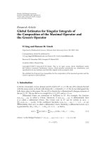
Figure 8 shows the performance results for RND(1024,
512). It is evident that the performance of the proposed
learning-based algorithm outperforms that of the average
decoder in the error-floor region. At low SNR region, average
decoding algorithm is better than the proposed algorithm.
The reason is due to the few occurrences of constant trapping
sets in the low SNR region. As SNR increases, constant error
frames increase until they become dominant in error-floor
region. The proposed algorithm on top of average decoding

shows the best results in all SNR regions. This is because
it combines the advantages of the two algorithms: learning-
based and average decoding as it improves both constant and
nonconstant type of patterns.
Figures 9 and 10 show the performance results for
the two LDPC codes, PEG(100,50) and PEG(1024,512).
10
−4
10
−5
10
−6
10
−7
10
−8
10
−9
Frame error rate (FER)
55.566.57
SNR (dB)
Conventional BP decoding algorithm
Average decoding algorithm
Proposed algorithm
Proposed algorithm on top of average decoding
Figure 9: Performance results for PEG(100,50) LDPC code.
10
−3
10
−4

10
−5
10
−6
10
−7
Frame error rate (FER)
2.52.75 3 3.25
SNR (dB)
Conventional BP decoding algorithm
Average decoding algorithm
Proposed algorithm
Proposed algorithm on top of average decoding
Figure 10: Performance results for PEG(1024,512) LDPC code.
While there is significant improvement for the proposed
algorithm in PEG(100,50), there is almost no improve-
ment in PEG(1024,512). The low improvement gain in
PEG(1024,512) is due to the low percentage (not more than
8%) of trapping sets that cause constant error patterns.
However, it is hard to implement PEG(1024,512) codes using
fully parallel architectures. As can be seen from the PEG code
construction algorithm [7], when a new connection is to be
added to a variable node, the selected check node for con-
nection is the one in the farthest level of the tree originated
Esa Alghonaim et al. 11
10
−3
10
−4
10

−5
10
−6
10
−7
Frame error rate (FER)
2.52.75 3 3.25
SNR (dB)
Conventional BP decoding algorithm
Average decoding algorithm
Proposed algorithm
Proposed algorithm on top of average decoding
Figure 11: Performance results for HE(1024,512) LDPC code.
Table 3: Results after the learning phase of HE(1024,512) LDPC
code.
i
TS
i
size TS
i
weight
ω
j
1
(8,2) 106
0%
2
(8,2) 49
0%
3

(12,2) 13
0%
4
(10,3) 9
1%
5
(8,3) 8
2%
6
(10,2) 7
0%
7
(7,3) 5
2%
8
(7,3) 5
3%
9
(7,3) 4
0%
10
(15,2) 3
0%
Table 4: Identified trapping sets and configuration percentages for
different LDPC codes.
CODE #TS %V %C
HE(1024,512) 55 27.15% 13.46%
RND(1024,512) 50 18.46% 9.9%
PEG(1024,512) 8 6.74% 3.42%
PEG(100,50) 57 60% 31.67%

MacKay(204,102) 40 50% 27.94%
from the variable node. This results in interconnections even
denser than pure random construction methods.
Figure 11 shows the performance for an interconnect
efficient LDPC code, HE(1024,512) [12], that has been
implemented in a fully parallel hardware architecture. This
LDPC code is designed to have a balance between decoder
throughput and error performance. The figure shows that the
10
−1
10
−2
10
−3
10
−4
10
−5
10
−6
10
−7
10
−8
Frame error rate (FER)
34 56
SNR (dB)
Conventional BP decoding algorithm
Average decoding algorithm
Proposed algorithm

Proposed algorithm on top of average decoding
Figure 12: Performance results for MacKay(204,102) LDPC code.
best performance is obtained using the proposed algorithm
on top of the average decoding algorithm. The performance
at 3.25B is not drawn due to the excessive simulation time
needed at this point.
Based on the results of all simulated codes, it is clearly
demonstrated that the application of the proposed algorithm
on top of average decoding achieves significant performance
improvements in comparison with conventional LDPC
decoding. In particular, one can observe that performance
improvements are highlighted for LDPC codes with relatively
low performance using conventional LDPC decoder. This
allows LDPC code design techniques to relax some of
the design constraints and focus on reducing hardware
complexity such as creating interconnect-efficient codes.
Ta ble 3 lists part of the trapping sets that are identified
during the learning phase of the HE(1024,512) LDPC
code. The complete number of identified trapping sets
is 55. One may note that trapping sets with the highest
weights have small number of variable and odd-degree check
nodes. Ta b le 4 shows the number of identified trapping sets
and percentage of check and variable nodes configured to
perform neutralization messages forwarding. It is clear that
only a subset of the variable and check nodes is configured,
which further decreases hardware cost.
6. CONCLUSION
In this paper, we have introduced a new technique to enhance
the performance of LDPC decoders especially in the error
floor regions. This technique is based on identifying trapping

sets of constant error pattern and reducing their negative
impact by neutralizing them. The proposed technique, in
addition to enhancing performance, has simple hardware
architecture with reasonable overhead. Based on extensive
12 EURASIP Journal on Wireless Communications and Networking
simulations on different LDPC code designs and sizes, it
is shown that the proposed technique achieves significant
performance improvements for: (1) short LDPC codes, (2)
LDPC codes designed under additional constraints such as
interconnect-efficient codes. It is also demonstrated that the
application of the proposed technique on top of average
decoding achieves significant performance improvements
over conventional LDPC decoding for all of the investigated
codes. This makes LDPC codes even more attractive for
adoption in various applications and enables the design
of codes that optimize hardware implementation without
compromising the required performance.
ACKNOWLEDGMENT
The authors would like to thank King Fahd University
of Petroleum & Minerals for supporting this work under
Project no. IN070376.
REFERENCES
[1]R.G.Gallager,Low Density Parity-Check Codes, MIT Press,
Cambridge, Mass, USA, 1963.
[2] T. Richardson, “Error floors of LDPC codes,” in Proceedings
of The 41st Annual Allerton Conference on Communication,
Control, and Computing, Monticello, Ill, USA, October 2003.
[3] E. Cavus and B. Daneshrad, “A performance improvement
and error floor avoidance technique for belief propagation
decoding of LDPC codes,” in Proceedings of the 16th IEEE

International Symposium on Personal, Indoor and Mobile Radio
Communications (PIMRC ’05), vol. 4, pp. 2386–2390, Berlin,
Germany, September 2005.
[4] T. Tian, C. Jones, J. D. Villasenor, and R. D. Wesel, “Con-
struction of irregular LDPC codes with low error floors,” in
Proceedings of the IEEE International Conference on Commu-
nications (ICC ’03), vol. 5, pp. 3125–3129, Anchorage, Alaska,
USA, May 2003.
[5] T. Tian, C. R. Jones, J. D. Villasenor, and R. D. Wesel, “Selective
avoidance of cycles in irregular LDPC code construction,”
IEEE Transactions on Communications, vol. 52, no. 8, pp. 1242–
1247, 2004.
[6] S. Gounai, T. Ohtsuki, and T. Kaneko, “Modified belief
propagation decoding algorithm for low-density parity check
code based on oscillation,” in Proceedings of the 63rd IEEE
Vehicular Technology Conference (VTC ’06), vol. 3, pp. 1467–
1471, Melbourne, Australia, May 2006.
[7] X Y. Hu, E. Eleftheriou, and D M. Arnold, “Progressive edge-
growth Tanner graphs,” in Proceedings of the IEEE Global
Telecommunicatins Conference (GLOBECOM ’01), vol. 2, pp.
995–1001, San Antonio, Tex, USA, November 2001.
[8] S. L
¨
andner and O. Milenkovic, “Algorithmic and combinato-
rial analysis of trapping sets in structured LDPC codes,” in
Proceedings of the IEEE Internat ional Conference on Wireless
Networks, Communications and Mobile Computing (Wirless-
Com ’05), vol. 1, pp. 630–635, Maui, Hawaii, USA, June 2005.
[9] G. Richter and A. Hof, “On a construction method of irregular
LDPC codes without small stopping sets,” in Proceedings of the

IEEE International Conference on Communications (ICC ’06),
vol. 3, pp. 1119–1124, Istanbul, Turkey, June 2006.
[10] D. J. C. MacKay, “Good error-correcting codes based on very
sparse matrices,” IEEE Transactions on Information Theory, vol.
45, no. 2, pp. 399–431, 1999.
[11] W. Ryan, “A Low-Density Parity-Check Code Tutorial, Part
II—the Iterative Decoder,” Electrical and Computer Engineer-
ing Department, The University of Arizona, Tucson, Ariz,
USA, April 2002.
[12] M. Mohiyuddin, A. Prakash, A. Aziz, and W. Wolf, “Synthesiz-
ing interconnect-efficient low density parity check codes,” in
Proceedings of the 41st Annual Design Automation Conference
(DAC ’04), pp. 488–491, San Diego, Calif, USA, June 2004.
[13] E. Alghonaim, A. El-Maleh, and M. Adnan Al-Andalusi,
“Parallel computing platform for evaluating LDPC codes per-
formance,” in Proceedings of the IEEE International Conference
on Signal Processing and Communications ( ICSPC ’07),pp.
157–160, Dubai, United Arab Emirates, November 2007.
[14] D. C. Mackay codes, />mackay/codes/.