Báo cáo hóa học: " Research Article Examining the Viability of Broadband Wireless Access under Alternative Licensing Models in the TV Broadcast Bands" docx

Hindawi Publishing Corporation
EURASIP Journal on Wireless Communications and Networking
Volume 2008, Article ID 470571, 12 pages
doi:10.1155/2008/470571
Research Article
Examining the Viability of Broadband Wireless Access under
Alternative Licensing Models in the TV Broadcast Bands
Timothy X. Brown and Douglas C. Sicker
Interdisciplinary Telecommunications Program, University of Colorado, Boulder, CO 80309-0530, USA
Correspondence should be addressed to Timothy X. Brown,
Received 5 June 2007; Accepted 25 January 2008
Recommended by Milind Buddhikot
One application of cognitive radios is to provide broadband wireless access (BWA) in the licensed TV bands on a secondary
access basis. This concept is examined to see under what conditions BWA could be viable. Rural areas require long range
communication which requires spectrum to be available over large areas in order to be used by cognitive radios. Urban areas
have less available spectrum at any range. Furthermore, it is not clear what regulatory model would best support BWA. This paper
considers demographic (urban, rural) and licensing (unlicensed, nonexclusive licensed, exclusive licensed) dimensions. A general
BWA efficiency and economic analysis tool is developed and then example parameters corresponding to each of these regimes are
derived. The results indicate that an unlicensed model is viable; however, in urban areas spectrum needs can be met with existing
unlicensed spectrum and cognitive radios have no role. In the densest urban areas, the licensed models are not viable. This is
not simple because there is less unused spectrum in urban areas. Urban area cognitive radios are constrained to short ranges and
many broadband alternatives already exist. As a result the cost per subscriber is prohibitively high. These results provide input to
spectrum policy issues.
Copyright © 2008 T. X. Brown and D. C. Sicker. This is an open access article distributed under the Creative Commons
Attribution License, which permits unrestricted use, distribution, and reproduction in any medium, provided the original work is
properly cited.
1. INTRODUCTION
Cognitive radios (CRs) have the potential for providing
broadband wireless access (BWA) as an alternative to existing
broadband options. In the Notice of Proposed Rule Making,
UnlicensedOperationintheTVBroadcastBands, the FCC

proposed both low- and high-power cognitive radio alter-
natives in the TV bands [1]. The latter can provide BWA
via outdoor access points (AP) to individual customers. A
standard for BWA in the TV bands is already being developed
by the IEEE in the event when such rules are made [2].
In urban areas, CR-based BWA is a potential competitor to
cable, DSL, and wireless options in the unlicensed bands
[3]. In rural areas, the better propagation at TV-band
frequencies below 1 GHz may provide a low-cost option for
BWA. In this paper, we test these potential outcomes via a
combined technical and economic analysis tool for BWA.
Unlike more technical analysis (e.g., see [2]), we examine the
economics of providing CR-based BWA in urban and rural
environments. In urban environments, there is relatively
little unused spectrum in the TV bands. However, customer
density is high, so the system can operate using short-range
access points (APs) and have large reuse. In rural areas,
the available spectrum is greater. However, APs need to use
longer ranges to efficiently cover the sparse customers. Long-
range transmitters may find many channels excluded because
of potential interference with distant TV coverage areas.
A further nuance to CR BWA deployment is the reg-
ulatory regime under which it operates. Access to the TV
spectrum is controversial [4] and several alternatives have
been proposed [5], that is, commons and property rights
models. To capture this range, we examine several unlicensed
and licensed regimes. In an unlicensed regime, spectrum is
free, but the CR must contend with other users who may
or may not have compatible architectures. In an exclusive
licensed regime, the CR BWA operator must pay for the

spectrum and can plan efficient use of the spectrum. In
between is a nonexclusive licensed regime where different
licensed CR operators pay for access to the spectrum and may
be required to cooperate with each other. We do not dwell
in this paper on the likelihood or mechanism through which
any of these regimes would be realized. Rather, we investigate
the impact of each of these regimes on the economics and
spectrum needs of BWA.
2 EURASIP Journal on Wireless Communications and Networking
In this paper, we develop a general purpose BWA spec-
trum requirements and economics tool. With this tool, we
examine the network cost for deploying a BWA network
in the six combinations of demographics (urban, rural)
and licensing (unlicensed, nonexclusive licensed, exclusive
licensed). For each of these regimes, parameters are esti-
mated. The resulting spectrum requirements and cost of
each regime indicates its relative viability. This paper extends
[6], by providing sensitivity analysis of key parameters. We
start by providing an overview of the BWA communication
architecture and a description of each regime.
2. COMMUNICATION ARCHITECTURE
The primary purpose of the BWA system is to provide
connectivity between the user stations and the Internet. The
BWA system consists of one or more access points (AP) that
communicate with fixed user stations. Multiple APs may be
needed to provide sufficient coverage or to provide sufficient
capacity similar to a cellular system. The AP may consist
of one or more antennas each covering different directions.
Radio channels are reused over the coverage area.
The user traffic from each AP needs to be backhauled to a

single or a small number of Internet gateways. The backhaul
channels can be wired or wireless. Thus the spectrum
requirements can be divided into access spectrum between
users and the AP and backhaul spectrum between the AP and
the Internet gateways.
The APs communicate to users over links that may
pass through or around man-made clutter, vegetation, and
terrain. For such links, frequencies below 3 GHz are most
suitable [7]. However spectrum below 3 GHz is less plentiful
compared to higher frequency spectrum. Since TV bands
are below 1 GHz and potentially have large tracts of unused
spectrum, they are especially suitable. The backhaul links
are more likely to be line of site since APs are mounted
higher and the Internet gateways can have dedicated towers.
Such links can be provided using higher frequencies, above
3 GHz, where unlicensed spectrum is plentiful and dedicated
high-capacity microwave links are available. For instance,
this is the approach used in the Philadelphia municipal BWA
system [8]. Therefore, in this paper we assume that the
backhaul spectrum needs (if any) are met with the readily
available higher frequencies and we focus on the access
spectrum needs.
For this paper, the BWA system uses unused spectrum in
the TV bands for its access spectrum. We focus on the United
States, however the analysis framework applies more broadly
to other countries as well. The BWA system must avoid inter-
fering with the licensed broadcast uses of the spectrum. The
APs in the BWA system use any of a number of techniques to
identify unused spectrum. To be specific, we assume that they
use a combination of geolocation and access to a database as

described in [9]. The user stations are controlled by the AP
and only transmit as permitted by the AP.
3. SIX REGIMES
We describe the six regimes and six factors which distinguish
them. The six regimes we consider vary across demographic
(urban, rural) and licensing (unlicensed, nonexclusive
licensed, exclusive licensed) dimensions.
3.1. Demographic and licensed regimes
We explore two aspects that follow from this cognitive radio
usage of the spectrum. First, the available spectrum varies
from place to place. Areas that have fewer licensed users
will have more potential spectrum for BWA. The question
is whether the available spectrum is sufficient for a viable
BWA system. To explore this aspect, we will investigate rural
and urban areas. As a limit, we consider two extremes: New
York City, one of the busiest television broadcasting regions
in the country; and Buffalo County South Dakota, noted as
being sparse. (Buffalo county, SD was chosen since it has the
lowest median per capita income among all US countries. It
is a candidate for using BWA to close the digital divide.)
The second aspect to BWA access to the TV spectrum
is that the licensing regime for this secondary access has
not been finalized and we seek to understand how different
licensing regimes could impact the BWA service. Unlicensed
access to the spectrum enables many users and potentially
uncoordinated services to be offered. Barriers to new
entrants are low and the BWA radio would need to resolve
the uncoordinated contention for radio resources. At the
other extreme, the BWA may be given licensed and exclusive
access to the spectrum not being used by primary users. This

reduces competition at both a service level from other BWA
providers and a radio resource level from other contending
users. However, the exclusive access may require the BWA
provider to pay for the license, which would increase the
BWA service cost. As a third option, we consider offering
multiple licenses (nonexclusive licensing). These licenses
could take several forms, ranging from permission to access
the entire available unused spectrum to divide the spectrum
into specific blocks, which are licensed and used on an
exclusive basis. For our purposes, we consider this range
of options equivalent if the number of licensees is small. A
small number of licensees will be motivated to cooperate and
provide de facto divisions of spectrum in the case that no
specific exclusive block license is provided. The nonexclusive
license regime may require the BWA operator to pay for the
license.
3.2. Six factors
For the purposes of our analysis, the six regimes differ in
six factors: population density, transmission range, available
spectrum, traffic per person, spectral efficiency, and cost of
spectrum. These are divided along demographic and license
axis.
Urban and rural areas, by definition, differ in population
density. An urban area can have densities over 4,000 people
per square kilometer and a rural area under 10 people per
square kilometer [10].
Generally, to be more efficient, rural systems will require
APs to have longer range in order to efficiently reach the
population. In urban areas, the AP can be mounted on
existing structures and, as described later, a short range

such as 500 m is both achievable and sufficient. In rural
T. X. Brown and D. C. Sicker 3
50
40
30
20
10
0
1 10 100 1000
Buffalo, SD
New York, NY
Interference radius (km)
Whitespace TV channels
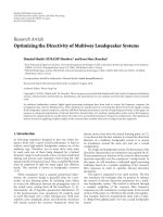
Figure 1: The number of 6 MHz TV channels available for cognitive
radio use as a function of potential interference. Computed for
New York City (Times Square) and Buffalo County, SD (geographic
center).
areas, APs will be mounted on higher towers to achieve
longer ranges. As an example, 10 km would be a reasonable
target. The choice of range depends on the availability of
spectrum in the vicinity of the BWA transmitters. Longer
transmission range requires spectrum to be available over
longer distances. This issue is addressed below. Population
density and transmission range together affect the number
of people captured by a single AP. However, their affects are
counterbalancing. As an example, rural areas may have 400
times smaller density, D, while the range, r ,canbe20times
larger so that r
2
is 400 times larger. In this case, they would

exactly counterbalance each other so that a rural AP and an
urban AP capture the same population.
A key factor in BWA viability is the availability of
spectrum. The appendix describes a method for estimating
the unused spectrum, also known as “whitespace.” Figure 1
shows the availability of unused TV channels as a function
of the interference radius of the CR. The interference radius
can be significantly larger than the transmission range of
the CR due to TV receivers’ sensitivity to interference. The
appendix estimates that the interference range is 10 times the
transmission range. From Figure 1, a transmission range of
500 m (5 km interference range) in New York would yield
4 unused channels (24 MHz). In Buffalo, SD a transmission
range of 10 km (100 km interference range) would yield 32
unused channels (192 MHz). The exclusive licensed model
would make this spectrum available to the BWA operator.
The unlicensed and nonexclusive licensed model would
divide the spectrum between different operators.
The unlicensed model can be supported by other
unlicensed spectrum below 3 GHz. There is 109.5 MHz of
useful spectrum, that is, 26 MHz at the 902–928 MHz and
83.5 MHz at 2.4–2.4835 GHz. Other unlicensed spectrum is
available but it is not useful for this application because of the
small size of the bandwidth block, limits on power, or limits
on usage.
The trafficperperson,U, represents the total traffic
demanded on the BWA system divided by the total popu-
lation. It is affected by both the licensing and demographic
regimes. In urban areas, BWA is one of several existing broad-
band delivery modes. In rural areas the major competitor

is satellite. Compared to satellite, BWA has the potential to
provide significantly lower delays and greater bandwidth. As
a result, BWA’s relative market share for broadband access
will be more in rural areas than in urban areas. If unlicensed
or nonexclusive licenses are used, then there will be lower
barriers to entry for BWA competitors and the market share
for each BWA provider will be less. The trafficperperson
affects the amount of spectrum required. More user traffic
per person requires more spectrum.
Spectral efficiency, E, captures the ratio of system traffic
to required spectrum to carry that traffic. It will depend
on whether unlicensed or licensed access will be granted.
With unlicensed spectrum, the BWA operator must contend
with other uncoordinated spectrum users. More robust but
less efficient transmission schemes are required in this case,
which lowers the spectral efficiency and accordingly increases
the required spectrum. Though the unlicensed approach
may require more spectrum, unlicensed spectrum promotes
competition and supports multiple service providers without
requiring any additional spectrum. Moreover, unlicensed
spectrum promotes innovation since it presents lower bar-
riers to diverse new services and applications. Further, in
the future if the BWA service becomes less viable, then
the unlicensed spectrum will already be available for other
uses, providing a natural technology evolution path without
protracted spectrum reassignment periods. Thus increased
spectrum requirements are traded against the reduced
administrative burden and operator flexibility when using
unlicensed access.
Spectrum cost depends on the licensing and demo-

graphic regimes. Unlicensed spectrum has no direct cost
to the BWA operator. Based on recent history, the licensed
regimes will require the BWA operator to pay some cost
in proportion to the population and the bandwidth of the
spectrum. This cost has been determined through spectrum
auctions. In these auctions, the cost of rural spectrum is
often much lower than urban spectrum. Lower spectrum
cost tends to lead to more spectrum usage; however, more
spectrum is available.
To make the different regimes and factors concrete, the
next section develops a tool for assessing the persubscriber
cost and required spectrum.
4. SPECTRUM REQUIREMENTS
We now present three approaches to determine the required
spectrum. When deploying a network, two major design
constraints dominate design—cost and usage. Engineering
the design of a network generally requires minimizing the
cost of the system, while ensuring the operational demands
can adequately be maintained. We use these principles
to inform our approach in defining the overall spectrum
requirements.
The first approach is based on a required service data
rate. The amount of spectrum required at an AP to provide
this rate to a user is a lower bound on the required spectrum.
4 EURASIP Journal on Wireless Communications and Networking
We denote this as the minimum service rate spectrum
requirements (MSR). The second approach is based on
minimizing the number of APs. Fewer APs lowers the system
cost, while requiring more spectrum to be able to carry
the greater traffic load on each AP. We denote this as the

minimum system cost spectrum requirement (MSC). MSR
and MSC set upper and lower bounds on the required
spectrum. Within these bounds, an operator will minimize
the overall cost to build their system. The third approach
analyzes the total capacity required by the system to carry
every user’s average traffic load. In principal this capacity
can be provided with any amount of spectrum. However,
to have sufficient total capacity there is a trade off between
the amount of spectrum and number of APs. As the amount
of spectrum decreases, the number of APs and the cost of
the system increase. Thus it becomes a tradeoff between
available spectrum and cost of providing the service. Based
on the value placed on the spectrum used, we can determine
a spectrum that minimizes the total cost of the BWA
deployment and spectrum. We denote this as the minimum
total cost spectrum requirements (MTC).
4.1. Key factors
The key factors in the model are described in detail in this
section.
Spectrum efficiency factors
A number of wireless technologies are in place today for
providing BWA. The IEEE 802.11a/b/g family of protocols
provides a range of communication capabilities with rates
from 1 up to 54 Mbps. The 802.16 family of protocols provide
data rates up to 134 Mbps. These technologies can use more
or less spectrum to increase or decrease communication
rates. The 802.16 standards work at a variety of spectral
bandwidths with proportional variations in channel rates.
An AP with more than one wireless interface working on
different channels will also have more capacity. Two or

more interfaces will yield a proportional two or more factor
increase in capacity. These observations suggest that a single
AP can use whatever spectrum is made available to it and
the useable channel rate is proportional to the spectrum
assigned. We denote the ratio of channel rate to spectrum
assigned as the spectral efficiency. Given these observations,
an AP can provide a rate B
= SE,whereB is the data rate (in
bps), S is the spectrum (in Hz), and E is the spectral efficiency
(in bps/Hz).
The spectral efficiency is a function of several factors
E
= e
modulation
e
reuse
e
protocol
e
loading
e
sharing
. The modulation
efficiency, e
modulation
, is the ability of a modulation scheme
to produce a bit rate in a given channel bandwidth, in
(bps/Hz). The reuse efficiency factor, e
reuse
≤ 1, accounts

for the fact that channels may not be used at every AP
due to cochannel interference between adjacent AP. The
protocol efficiency factor, e
protocol
≤ 1, accounts for the
overhead of packet headers and channel access. The loading
efficiency factor, e
loading
≤ 1, accounts for the level to which
a channel can be loaded in the long term and still experience
good performance. Too high a loading leads to excessive
queuing and delays. The minimum service rate model
considers only the peak rate and so loading is not relevant
(e
loading
= 1). The sharing factor, e
sharing
≤ 1, accounts
for additional overhead to resolve contention between the
different coexisting operators in the same band.
Access point cost
The cost of building the BWA network infrastructure and
paying for it depends on the cost of the AP and the cost of
terminating to the Internet. For these costs, we consider the
net present value costs with discount factor d (A discount
factor of d means that a cost of x dollars y years in the future
has NPV of x(1
− d)
y
. Given an ongoing cost stream of x

dollars per year and discount factor of d, the NPV of this
stream is x/d.).
For the AP, this is the initial cost of the hardware
and installation, and the discounted cost of the future
maintenance and operations expenses
K
ap
= k
f
+
k
om
d
,(1)
where k
f
is the initial fixed hardware and installation costs
and k
om
is the annual operations and maintenance costs.
Traffic per person
Active BWA users can generate significant traffic. However,
these users may be a fraction of the total population
depending on a number of factors. Let U be the traffic
per person where U
= u
traffic
u
active
u

takeup
u
mrktshr
u
operator
.
The traffic per active user, u
traffic
, is the average usage of
such a user over the busy hour in bps. It includes the
total of uplink and downlink traffic.Theactiveuserfactor,
u
active
≤ 1, is the average fraction of users that are active
during the busy hour. The take up factor, u
takeup
≤ 1, is
the ratio between the number of broadband users and the
total population. The market share factor, u
mrktshare
≤ 1, is
the fraction of broadband users that are users of BWA. The
operator factor, u
operator
≤ 1, is the fraction of the BWA
market captured by one BWA operator. A BWA operator has
u
takeup
u
mrktshare

u
operator
customers (as a fraction of the total
population) which are generating u
traffic
u
active
bits per second
of traffic on average in the busy hour.
4.2. Minimum service rate spectrum requirements
Broadband service providers often specify a service rate that
they are providing to users, such as 1.5 Mbps DSL or a
27MbpsCablemodem.Thisrateisthepeakrateatwhich
users can exchange data with their service provider. This
rate is typically shared among different users and individual
users can have average rates that are only a fraction of this
carrier specified rate. However, this specified rate is often
a criterion in comparing different service offerings. The
minimum service rate spectrum requirements model relates
a specified minimum service rate offered to users, denoted
as the user bandwidth, B
U
, and the spectrum required to
T. X. Brown and D. C. Sicker 5
provide this bandwidth at each AP. Given a total spectrum
S, the user bandwidth per AP is B
AP
= SE. This bandwidth
must be shared by all users in practice, but defines the peak
usable rate any customer could hope to achieve. Thus the

required spectrum is
S
MSR
=
B
U
E
(MSR spectrum requirement), (2)
where S
MSR
is the required spectrum (in Hz, Hertz), B
U
is
the user bit rate per user (in bps, bits per second), and E is
the spectral efficiency of the radio system (in bps/Hz). The
MSR spectrum requirement does not depend on the number
of APs or user traffic for the covered area.
4.3. Minimum system cost spectrum requirements
We define the maximum spectrum that can be usefully
exploited to carry a given traffic load per user. As will be seen
in Section 4.4, the NPV cost of the BWA system decreases
with additional spectrum. To a first order, more spectrum
meansthateachAPcancarrymoreloadandsofewerAPs
are needed, which lowers the overall system cost. However,
coverage requires a minimum number of APs (N
min
)to
provide service over the metropolitan area, A:
N
min

=
A
πr
2
,(3)
where πr
2
is the maximum coverage area of an AP. The
minimum cost system will have N
min
APs. How much
spectrum is required for these few APs? If U is the average
traffic per person in the busy hour and D is the population
density, then a single AP captures at most UDπr
2
traffic. The
bandwidth capacity per AP is SE.Thus,
S
MSC
=
U · D · πr
2
E
(MSC spectrum requirement). (4)
This incorporates the number of APs and required traffic
capacity.
4.4. Minimum total cost spectrum requirements
The MSR and MSC spectrum requirements are sufficient
if spectrum cost is not considered. The required spectrum
is simply the maximum of S

MSR
and S
MSC
. The second is
more important since the minimum system cost is typically
reached with a large S
MSC
. However, there may be limited
spectrum available. Even if unlimited spectrum is available,
there may be a cost to this spectrum. In this case, the BWA
operator will trade the savings in fewer APs against the cost
of more spectrum.
We first introduce a system cost model. We then
introduce the spectrum cost and determine what spectrum
is required to minimize the total cost of the system and
spectrum. The costs only consider the system and spectrum
costs. The customer costs of Internet backhaul, marketing,
billing, customer service, and customer premises equipment
are a significant portion of the service cost. However, these
costs are independent of the spectrum and so are not
included.
System cost
The system cost, to a first order, is proportional to the
number of APs. For a total spectrum, S, the data rate per AP
is again SE. It follows that to provide UP total capacity to a
total population, P, requires the following number of APs:
N
=
UP
SE

. (5)
Thus the system cost per person is
K
Sys
(S) =
NK
ap
P
=
UK
ap
SE
. (6)
This shows that the cost of the system is directly propor-
tional to the traffic generated per user.
The system cost decreases monotonically as S increases.
However, the number of APs is lower bounded by N
min
and so the cost is minimized at S
MSC
as computed earlier.
Additional spectrum only serves to increase the data rates
experienced by users without changing the system costs.
Spectrum cost
Spectrum is valued in a number of ways. In this study, we use
K
S
to denote the cost of one unit of spectrum (e.g., one MHz)
for an area divided by the population of that area (dollars per
MHzpop).Thetotalsystemandspectrumcostperpersonis

then
K
T
(S) = K
Sys
(S)+K
S
S. (7)
The amount of spectrum that minimizes this cost can be
found by standard minimization techniques with the result
S
MTC
=

UK
ap
EK
S

1/2
(MTC spectrum requirement).
(8)
This requirement incorporates the user traffic, spectrum effi-
ciency, and cost factors. However, the square root decreases
the sensitivity to these factors.
4.5. Variable sensitivity
The three spectrum models are sensitive to the variables that
are assumed. All of the models depend on the spectrum
efficiency, E, and its constituting factors. The first two
models are directly sensitive. A factor of two change in the

spectrum efficiency yields a factor of two change in the
required spectrum. The last two models depend on the user
bandwidth, U, and its constituting factors. The relationship
is linear for the MSC model and sublinear for the MTC
model.
The required user bandwidth, B
U
,affects only the MSR
model and the effect is linear. The max population covered
by an AP, Dπr
2
,affects only the MSC model and the effect is
linear. However, D and r tend to have a negative correlation
that reduces the impact of these factors. The cost factors only
affect the MTC model and have a sublinear relationship.
6 EURASIP Journal on Wireless Communications and Networking
Table 1: Output variables.
Var ia ble
Description
S
Total spectrum required for all BWA operators
N
Total number of APs per 1000 km
2
for all BWA
operators
B
AP
Bandwidth capacity provided by each AP
K

Sys
(S)
System cost per subscriber
K
T
(S)
Total cost per subscriber
Table 2: Output spectrum requirements.
Variable Description
S
MSR
Spectrum required to provide a minimum service rate
S
MSC
Spectrum required to minimize system cost
S
MTC
Spectrum required to minimize total system cost
4.6. Analysis outputs
The analysis can be summarized via the output variables
and output spectrum requirements in Tables 1 and 2.The
spectrum is the required spectrum according to each model.
The number of APs is based on assuming an area of A
= 1000 km
2
. This area is large compared to most cities
and small compared to most rural areas, but it provides a
common point of reference. The number of APs indicates the
system infrastructure required. The spectrum and number of
APs as computed in the previous section are per operator. In

order to correctly reflect the total spectrum and number of
APs, we need to incorporate the number of BWA operators.
If S and N are the per operator requirements, then S/u
operator
and N/u
operator
arethetotalrequirementsforallBWAusers.
The bandwidth capacity per AP indicates the bandwidth
required to provide sufficient traffic capacity. It is always
at least B
U
. Though the models considered cost factors to
different degrees, we compute the system and total costs
for each method. Cost per person is converted to cost per
subscriber to give a better indication of what costs will
be from a network operator’s perspective. If K is a cost
per person, then K/( u
takeup
u
mrktshr
u
operator
) is the cost per
subscriber. We reiterate that these costs consider network
costs and do not include customer equipment and marketing
costs.
As a final comparison, we consider a startup system
model. The startup system model uses spectrum as deter-
mined by the minimum service rate model, S
MSR

,and
enough APs to provide coverage, that is, N
min
. This system
does not consider the user traffic. It is the lowest cost system
that could be built and start to provide service. The cost
per subscriber is calculated as described above. However, this
is the cost per eventual subscriber since the startup system
would need to invest in additional APs in order to have
enough capacity to carry these subscribers’ traffic.
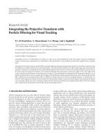
4.7. Analysis summary
The interaction between the different models is seen in
Figure 2.InFigure 2(a), the relationship between the min-
1000
100
10
1
0.1
0.1 1 10 100
Required spectrum (MHz)
Minimum service rate (Mbps)
8MHz
(a)
100000
10000
1000
100
10
Subscriber ($)
1 10 100 1000

$900
22 MHz
To t a l
Spectrum
System
Minimum
system cost
upper limit
Minimum
service rate
lower limit
To t a l sp e c t r u m ( M H z )
(b)
Figure 2: Example derivation. The minimum service rate spectrum
requirements (a) sets a lower limit on the required spectrum
(8 MHz). The “knee” in the system cost (b) sets the upper limit on
the usable spectrum (63 MHz). The minimum total cost determines
the persubscriber cost and required spectrum ($900, 22 MHz).
imum bandwidth per user and the required spectrum is
plotted. For a given minimum required user bandwidth (e.g.,
1 Mbps), the minimum required spectrum is plotted (e.g.,
8 MHz). In Figure 2(b) this sets a lower limit on the required
spectrum. The minimum system cost sets an upper limit on
the usable spectrum (e.g., 63 MHz). The minimum of the
total cost within this range sets the overall minimum cost and
spectrum requirements (e.g., $900, 22 MHz).
5. EXAMPLE APPLICATION: INPUT VARIABLES
This section describes the input variables used in Section 6.
Many of the variables are based on the recent project to
provide a municipal wireless network in Philadelphia, USA

[8, 11].
5.1. Spectrum efficiency factors
A number of wireless technologies are in place today for
providing BWA. Cellular technologies are also available.
So-called CDMA 2000 and W-CDMA are third-generation
T. X. Brown and D. C. Sicker 7
Table 3: Modulation efficiency of several wireless technologies.
Technology
Channel bandwidth Channel rate Efficiency
(MHz) (Mbps) (bps/Hz)
802.11b
22 11 0.5
(WiFi) [13]
802.11a [13]20 542.7
802.16 [12] 28 134 4.8
CDMA-2000
1.25 3.1 2.5
EVDO [23]
technologies with data rates in the few megabits per second
range.
Ta ble 3 lists the modulation efficiency of a few wireless
technologies including wireless LAN (802.11b, 802.11a),
wireless MAN (802.16), and third generation cellular
(CDMA-2000 EVDO release 0). Spectral efficiencies range
from 0.5 to about 5 bps/Hz [12, 13]. These efficiencies
are best case efficiencies. For instance 802.11a can only
achieve its highest rate within about 10 meters of the access
point, whereas it can achieve lower rates to significantly
further distances. To account for this we downgrade the best
available efficiency by 50% in e

modulation
.
These rates are so-called channel rates and do not
include wireless protocol overhead, which reduces the usable
capacity. For instance, 802.11b has a maximum channel rate
of 11 Mbps, while the maximum usable capacity is about
3.5 Mbps. Overhead from other protocols (e.g., TCP/IP/LLC)
can reduce capacity further to below this rate. In other words,
the true capacity is about 30% of the channel rate [14].
Similar overhead can be observed in other protocols.
Beyond protocol inefficiencies, Internet applications gen-
erally perform better when the loading on the channel is
below full capacity. As the load approaches capacity, queuing
delays can develop that degrade the performance. For real-
time applications, such as voice, low delays are critical. For
more bursty applications such as Internet browsing, delays
are less critical. However, an average load below capacity is
necessary to avoid significant periods of congestion. With
such traffic, a high load, for example 50%, can result in
acceptable performance. This loading is the average over the
peak busy hour. Typical wireless access networks have much
lower loading over the day [15, 16]. Nevertheless, busy-hour
provisioning is necessary to provide adequate service.
The maximum raw channel rates are best-case rates for
dedicated spectrum. In shared or unlicensed environments,
the available channel rates are below these maximum rates
since the lower rates are more robust to radio noise and
interference. The ratio of the lower rate used for the purposes
of providing more robust coverage to the maximum rate is
the sharing efficiency, e

sharing
. If dedicated spectrum is pro-
vided to a single operator to provide BWA, then e
sharing
= 1.
We assume that the nonexclusive licenses are well organized
so that e
sharing
= 1. Non-cooperative operators can choose
interfering channels. Even if cooperating, different operators
may cover the same area multiple times using incompatible
channel assignments. Besides other BWA operators, there
may be other services and applications that are not amenable
to coordination. Because of these inefficiencies more robust
modulation is necessary. The 802.11 standards are designed
to operate in unlicensed environments, while the 802.16
standards are designed for unlicensed and licensed with the
most efficient protocols designed for licensed. The maxi-
mum current 802.11 efficiency (2.7 bps/Hz) is approximately
half of the maximum 802.16 efficiency (4.8 bps/Hz). The
resulting sharing efficiency in shared unlicensed spectrum is
e
sharing
= 0.5.
The spectral efficiency above assumes that an operator
assigns different frequency channels to its nearby APs in
order to avoid interference. A simple strategy to achieve
this is to divide the spectrum into subbands and assign the
spectrum in a nonconflicting pattern. This pattern can be
repeated over the coverage area so that channels are reused

many times. This strategy is applied in cellular and wireless
LAN deployments. Cellular systems use a variety of reuse
patterns depending on the technology. For instance, the
entire spectrum is assigned to each AP in CDMA cellular
systems. This is traded against a lower net spectral efficiency.
Since WLAN technologies are most similar to the BWA
technologies, we will follow their reuse strategy, that is, a
reuse of three. Every AP would then have at most one third
of the total spectrum available.
In this study, we will assume a radio technology similar
to 802.16 that can utilize a variety of spectral bandwidths,
has a modulation efficiency of about e
modulation
= 2.5 bps/Hz,
aprotocolefficiency of e
protocol
= 0.30, and typically transmits
at one half of the maximum channel rate, e
loading
= 0.50. In
the minimum service rate model, e
loading
= 1.00. Channels
are reused in a pattern of three channels, e
reuse
= 0.33.
The sharing factor depends on whether channel access is
unlicensed, e
sharing
= 0.5, or licensed, e

sharing
= 1.00.
5.2. Access point costs
The access point costs can be divided into (a) costs that
are independent of the coverage and total usable bandwidth
per AP; (b) costs that depend on the coverage per AP;
and (c) costs that depend on the usable bandwidth per AP.
The model AP is based on the configuration to achieve
the minimum number of APs (i.e., have the maximum
coverage). It consists of a broadband wireless radio; a set
of 3 to 6 directional antennas either attached to an existing
structure or on a mast; additional radios as necessary for
wireless backhaul; and connections to power. As the coverage
decreases, it is possible to use lower power and less expensive
amplifiers. As the user bandwidth per AP decreases, the AP
can use fewer channels and fewer antennas to achieve its
capacity goal. This reduces the hardware and installation
cost. For simplicity we assume that the NPV cost of an AP
is independent of these capacity and coverage factors. For
instance, a rural AP will consist of a taller more expensive
mast than an urban AP. However, the site costs in urban
environments are higher. Based on data from Philadelphia,
the average installed cost of an AP is $5,000. The initial total
estimated capital cost in Philadelphia is $10 M, while the total
annual operating expenses are $8 M. If we assume these costs
8 EURASIP Journal on Wireless Communications and Networking
are proportional to the number of AP, the annual operating
costs per AP are 80% of the initial capital costs, or $4,000 per
AP. Given a discount factor of 20%, this indicates that the
NPV cost of each AP is K

AP
= $25,000.
5.3. Traffic per person
A BWA system might provide service to a variety of users
including residential, commercial, and municipal. The users
might access the BWA system for communication, web-
browsing, and media download applications. There may
be other embedded users including sensors, transaction
processing devices (e.g., parking meters), security video
cameras, and remotely controlled devices (e.g., sprinklers).
For simplicity, we consider a single typical subscriber which
generates trafficatarateofu
traffic
during the busy hour. This
traffic is the total of uplink and downlink bandwidths since
the capacity of many wireless protocols can be divided as
needed between up and down links. Separate up and down
link analysis is unnecessary. Applications such as voice over
IP use 10’s of kilobits per second (kbps). Web browsing
alternates between brief periods of high data rate downloads
and longer periods of viewing the content. Streaming video
or audio can be many 100’s of kbps. A remote video camera
can generate 300 kbps. These rates are growing over time.
These observations suggest that an active user in the near
future could generate 100 kbps of traffic on average during
the busy hour.
Users access the Internet at different times of the day.
In any given busy hour, only a fraction of the users may be
actively using the system. Internet access is a regular part of
many users’ daily activity and as many as 50% of the users

might be active during the busy hour.
Not every person in the population corresponds to a user.
Some people will not be able to afford or will not have the
need of a broadband service. Household members might
share the service. A household consists of 2.5 people on
average, suggesting that the take up rate is at most 100/2.5
= 40 lines per 100 people. The take up rate was 17 broadband
lines per 100 people at the beginning of 2006 and has been
growing steadily [17]. We extrapolate that, in the near future,
the take up rate will approach 25 broadband lines per 100
people.
Given the set of broadband users, only a fraction will use
a BWA service depending on the market share of the BWA
service provider. In rural areas, the primary competition to
BWA will come from satellite service and existing Wireless
ISPs based on the 2.4 GHz unlicensed bands. Because of
better coverage and more bandwidth, we expect the BWA
to have a competitive advantage over these alternatives
capturing a majority of the broadband users. The market
share in this case is 50%. In urban areas, there are additional
competitors such as DSL and Cable. These are already
entrenched. The BWA service will have lower market share
against these four competitors. The market share in this case
is 20%. This market share is for a single BWA operator.
If nonexclusive licenses or unlicensed access regimes are
used, then each BWA operator will enjoy half of this market
share.
10000 100000 1000000 10000000 100000000
10
1

0.1
Population
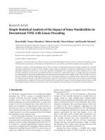
$ (MHzpop)
Figure 3: Normalized spectrum cost as a function of population for
full BTAs auctioned in the PCS broadband auction.
In this study, we assume an active user that generates
u
traffic
= 100 kbps in the busy hour. Half of these users are
active in the busy hour, u
active
= 0.50 and a fraction of the
population that is a user, u
takeup
= 0.25. The market share will
vary from u
mrktshare
= 0.20 to u
mrktshare
= 0.50 depending on
the regime. The operator fraction is u
operator
= 1.00 for the
licensed exclusive regime and u
operator
= 0.50 for the licensed
nonexclusive and unlicensed regimes.
We note the difference between our factors here and
the industry “over subscription factors.” A typical wireless
Internet service provider (WISP) will share an 11 Mbps link

between 100 users [18]. The over subscription factor of 100
is based on implicit assumptions about the average traffic
per user. In our model we make these assumptions explicit.
TocompetewithaWISP,theBWAserviceprovidermust
provide at least Mbps service to customers. We assume B
U
= 1 Mbps. This is the same target as in Philadelphia.
5.4. Spectrum cost
The cost of the spectrum can be estimated from recent
FCC auctions. The PCS broadband auction was both recent
and appropriate for a BWA service [19]. Figure 3 shows the
normalized cost (in $/MHz pop) as a function of the licensed
basic trading area (BTA) population (only includes full BTAs
for the full license size that actually were sold). Clearly, less
populated BTAs tend to have lower spectrum costs than more
populated areas. If we use BTAs with populations less than
100,000 to represent rural areas and BTAs with populations
more than 1,000,000 people to represent urban areas, then
we can estimate the relative spectrum cost. The average
normalized cost for the rural areas is $0.21 and for urban
areas is $1.01, or approximately $0.2 and $1.0, respectively.
5.5. Transmission range
A BWA system requires a minimum number of APs to
provide sufficient signal to reach the intended coverage area.
We assume frequencies are in the TV bands; the APs use high
gain antennas; in urban areas the APs are not placed on high
towers, the subscriber equipment uses an outdoor antenna;
and the transmit power is at least 1 W.
What kind of coverage can be expected under these
assumptions? Wireless links using 802.11 typically have

T. X. Brown and D. C. Sicker 9
Table 4: Regime independent input variables used in the model.
Var ia ble Value
Description
e
modulation
2.5 (bps/Hz)
Modulation efficiency
e
reuse
0.33
Frequency reuse factor
e
protocol
0.30
Protocol efficiency factor
e
loading
0.50
Network loading factor
k
f
$5,000
Fixed cost of an AP
k
om
$4,000
Annual operations and
maintenance cost per AP
d 20%

Discount factor for NPV
calculation
B
U
1Mbps
Minimum data bandwidth
per user
u
traffic
100 kbps
Tr afficrateofactiveuserin
busy hour
u
active
0.50
Fraction of users active in
busy hour
u
takeup
0.25
Take up fraction for
broadband service
specified outdoor ranges of 100 m or more [20, 21]. Exper-
iments have shown point-to-point links at distances of many
10’s of kilometers under line-of-site conditions with high-
gain antennas [21, 22]. Under more typical conditions with
APs placed on rooftops, the range can approach a few
kilometers. These data suggest that in urban areas high-gain
antennas placed at modest heights should enable ranges up to
500 m. In rural areas high towers and less urban clutter can

enable transmission ranges of 10 km. We emphasize that the
range limit is not purely a question of meeting the radio link
budget. A CR-based operator will use shorter ranges than
possible in order to avoid interference with TV reception
areas as described in the appendix. In any case, these ranges
are only a direct factor for the minimum system cost model.
For the other models, the number of access points is greater
than N
min
and the transmission range is set by other factors
than this minimum.
5.6. Model variables
The input variables that are independent of the regime are
summarized in Tabl e 4 . Five variables depend on the regime.
They are summarized in Tab le 5 .
6. EXAMPLE APPLICATION: OUTPUT VARIABLES
Based on the input variables derived in the previous section,
we apply the spectrum requirement and cost analysis to
provide some insights into the effect of each regime. The
output of the model is shown in Tables 6 and ?? and plotted
in Figure 4.
6.1. Rural areas
Rural areas have the potential to go to low system cost per
subscriber and exploit more than 300 MHz of bandwidth
if unlicensed. Given the more than 100 MHz of existing
unlicensed spectrum at 900 MHz and 2.4 GHz, the addition
of 100 MHz to 200 MHz can push the per subscriber cost
below $200 per subscriber.
If an exclusive license is used, then the total cost must
be considered if the operator must pay for the license. An

exclusive license would allow an operator to have a total
cost around $250. About 80 MHz would be required to
achieve that price. Many rural areas have this volume of
spectrum available. The nonexclusive license would require
more spectrum and would have a total cost over $300,
mainly because of the duplication of infrastructure implied
by having multiple operators.
In all scenarios, the effective per AP bandwidth shared
by subscribers would be 7 to 20 times the minimum
requirement of 1 Mbps. A startup system (Ta bl e 6 )couldbe
built for less than $100 per eventual subscriber if licensed, but
further investments would be needed to have the necessary
capacity.
6.2. Urban areas
In urban areas, an unlicensed approach requires more than
100 MHz in order to have a price below $400 per subscriber.
This much unlicensed spectrum already exists below 3 GHz.
In New York City the available whitespace bandwidth is
24 MHz. Going from the 110 MHz of existing spectrum to
the maximum useful spectrum of 127 MHz would yield a
14% reduction in cost. This modest savings must be weighed
against the added cognitive radio complexity to use the
whitespace bandwidth. This result follows from the relatively
short range of each AP and the low market share. As a result,
each AP can at best capture relatively few customers. Lack
of bandwidth is not directly the constraint. Longer range
AP could be used and that would increase the number of
customers captured per AP. However, only modest increases
are possible in urban areas such as New York before no
channel would be available (see Figure 1). The unlicensed

spectrum here is similar to the 80 MHz of access spectrum
used in the Philadelphia model. The cost per subscriber
is higher than Philadelphia. In our sample model, we are
assuming only a 20% market share for BWA split between
two operators. The Philadelphia model is more optimistic.
For instance, if the market share is the same but the operator
share rises to 100%, the required spectrum remains the same,
but the system cost is half.
Licensing helps by reducing the required bandwidth
to 22 MHz, an amount of white space available in many
markets. However, the persubscriber total costs are at best
$900 and unlikely to be viable. BWA via TV spectrum is
a late comer to the urban broadband market. The lack of
viability follows from its likely low market share. As shown
in Figure 5, it would require a market share of 65% of the
broadband market to drop below $500 per subscriber. Such
high market share is unlikely given the existing broadband
competitors. Even the startup system has a minimum cost
of around $250. Recall that the total cost as described here
does not include additional costs such as the subscriber
equipment and its installation.
10 EURASIP Journal on Wireless Communications and Networking
Table 5: Regime-dependent input variables.
Regime
Sharing efficiency
Spectrum cost
($/MHz-pop)
Operator share Market share Density pp/km
2
TX range

e
sharing
K
S
u
operator
u
mktshare
Dr
Rural
Unlicensed 0.5
0
50%
50% 10 10 km
Licensed nonexclusive 1.0
0.2
50%
Licensed exclusive 1.0
0.2
100%
Urban
Unlicensed 0.5
0
50%
20% 4,000 500 m
Licensed nonexclusive 1.0
1.0
50%
Licensed exclusive 1.0
1.0

100%
Table 6: Spectrum requirements and cost of a startup system.
Regime S MHz N per 1000 km
2
B
ap
Mbps K
Sys
$/sub K
T
$/sub
Rural
Unlicensed 8 3 1 $127 $127
Licensed nonexclusive 4 3 1 $127 $140
Licensed exclusive 4 3 1 $64 $70
Urban
Unlicensed 8 1273 1 $318 $318
Licensed nonexclusive 4 1273 1 $318 $480
Licensed exclusive 4 1273 1 $159 $240
Licensed nonexclusive
Unlicensed
Licensed
exclusive
Urban
Rural
Required spectrum (MHz)
Subscriber ($)
0
200
400

600
800
1000
1200
1400
0 100 200 300 400
Figure 4: Required spectrum and cost per subscriber in the six
regimes.
7. CONCLUSIONS
In this paper, we have presented a general analysis framework
for investigating the spectrum and cost issues associated with
building out a broadband wireless access network. Specif-
ically, we have examined under what conditions cognitive
radios could be viable to provide broadband wireless access
(BWA) in the licensed TV bands. We explored this issue
along demographic (urban, rural) and licensing (unlicensed,
nonexclusive licensed, exclusive licensed) dimensions. We
developed a general BWA efficiency and economic model
for this analysis and derived parameters corresponding to
each of these regimes. The results indicate that in rural areas
an unlicensed model is viable and the additional spectrum
would be useful despite existing unlicensed spectrum. A
0.1
0.2
0.4
0.7
1
0.1
0.2
0.4

0.7
1
Required spectrum (MHz)
Subscriber ($)
Licensed exclusive
Unlicensed
Market share0.1
10 100 1000
0
200
400
600
800
1000
1200
1400
Figure 5: Effect of market share on per subscriber cost and required
spectrum in the urban area.
licensed model is also viable, although at a higher cost. In the
densest urban areas no model is economically viable. This is
not simple because there is less unused spectrum in urban
areas. Urban area cognitive radios are constrained to short
ranges and many broadband alternatives already exist. As a
result either there is already sufficient unlicensed spectrum or
the cost per subscriber is prohibitive. An exclusive license is
a better choice than nonexclusive licenses. It results in lower
cost per subscriber and less required spectrum. The potential
for monopoly behavior is unlikely, given the competition
from other broadband access technologies. These results are
based on one set of input variables for the model. The model

can be easily manipulated to account for other scenarios or
different assumptions. These results provide useful input for
a variety of spectrum policy issues.
T. X. Brown and D. C. Sicker 11
Table 1: Output results in each regime.
Rural
(a)
Model S MHz
N per B
ap
K
Sys
K
T
$/sub
1000 km
2
Mbps $/sub
MSR 16 125 1 $2,500 $2,500
MSC 317 6 10 $127 $127
MTC n/a n/a n/a n/a n/a
(b)
Model S MHz
N per B
ap
K
Sys
K
T
$/sub

1000 km
2
Mbps $/sub
MSR 8 125 1 $2,500 $2,513
MSC 159 6 10 $127 $381
MTC 112 9 7 $180 $360
(c)
Model S MHz
N per B
ap
K
Sys
K
T
$/sub
1000 km
2
Mbps $/sub
MSR 4 125 1 $2,500 $2,506
MSC 159 3 20 $64 $318
MTC 79 6 10 $127 $254
Urbal
(d)
Model S MHz
N per B
ap
K
Sys
K
T

$/sub
1000 km
2
Mbps $/sub
MSR 16 20000 1 $2,500 $2,500
Unlicensed
MSC 127 2547 4 $318 $318
MTC n/a n/a n/a n/a n/a
(e)
Model S MHz
N per B
ap
K
Sys
K
T
$/sub
1000 km
2
Mbps $/sub
MSR 8 20000 1 $2,500 $2,662 Licensed
MSC 63 2547 4 $318 $1,588 Non-Exclusive
MTC 32 5085 2 $636 $1,271
(f)
Model S MHz
N per B
ap
K
Sys
K

T
$/sub
1000 km
2
Mbps $/sub
MSR 4 20000 1 $2,500 $2,581 Licensed
MSC 63 1273 8 $159 $1,428 Exclusive
MTC 22 3596 3 $449 $899
APPENDIX
AVAILABLE TV WHITESPACE
The TV Whitespace was assessed for this paper using a
FCC transmitter location database [24]. For each area of
study, a location was determined: 40 : 46 N, 73 : 58 W
for New York City and 44 : 03 N, 99 : 11 W for Buffalo
County, SD. Using the database, every TV transmitter was
identified within 1000 km. For each transmitter, the database
identifies the distance to the Grade B signal contour (The
Grade B contour is a regulatory concept that corresponds to
the approximate range of a TV signal.). For channels whose
contour encompasses the location, the distance is zero. For
each channel the closest signal contour is identified. Since
TV receivers are sensitive to both cochannel and adjacent
channel interference, for each channel the closest signal
contour on the same or adjacent channel is identified (noting
that some channels such as 13 and 14 are adjacent in number
but not frequency). This distance is the interference distance
for that channel. For any given distance, d, n(d) counts the
number of channels whose interference distance exceeds d.
This function is plotted in Figure 1.Thisisnotintended
to be a definitive assessment. It is not based on actual

measurements and does not include existing secondary uses
such as wireless microphones. However, it does suggest the
relative viability of cognitive radio use in rural and urban
environments.
How far must a BWA transmitter be from a TV receiver
at the edge of its coverage area? A cognitive radio that
is transmitting at a maximum range d, can potentially
interfere with TV receivers that are much farther than d away.
The interfering signal power at the Grade B contour must
be less than approximately
−100 dBm to avoid interfering
with TV reception [25]. Lognormal shadowing introduces
signal variability with a standard deviation of approximately
5 dB. If we include two standard deviations of shadow fade
margin, the required mean interfering signal power must be
less than
−110 dBm. The minimum receive threshold of a
typical 802.11 radio at an intermediate rate is approximately
−90 dBm. Freespace pathloss will introduce 20 dB of atten-
uation for each factor of 10 increase in transmitter distance.
In fact, long distant signals near the ground tend to suffer
a greater rate of attenuation so that this is conservative.
Thus using an interference distance, d,10timeslarger
than the range of the BWA transmitter will conservatively
produce interfering signals which are no more than
−90 dBm
(range of BWA transmitter)
−20 dB (additional attenuation
due to factor of 10 distance further away)
= −110 dBm as

required.
ACKNOWLEDGMENTS
The authors thank the useful conversations with Dale
Hatfield, Jim Snider, and Michael Calabrese. The work was
supported in part by NSF Grant CNS 0428887.
REFERENCES
[1] Federal Communications Commission, “Notice of proposed
rule making, unlicensed operation in the TV broadcast bands,”
FCC 04-186, May 2004.
[2] C. Cordeiro, K. Challapali, D. Birru, and N. Sai Shankar,
“IEEE 802.22: the first worldwide wireless standard based on
cognitive radios,” in Proceedings of the 1st IEEE International
Symposium on New Frontiers in Dynamic Spectrum Access
Networks (DySPAN ’05), pp. 328–337, Baltimore, Md, USA,
November 2005.
[3]D.Howard,“It’saWi-Fiworld.ACMnetWorker6,3,”
September 2002.
12 EURASIP Journal on Wireless Communications and Networking
[4] M. J. Marcus, “Unlicensed cognitive sharing of TV spec-
trumml: the controversy at the Federal Communications
Commission,” IEEE Communications Magazine, vol. 43, no. 5,
pp. 24–25, 2005.
[5] J. M. Peha, “Approaches to spectrum sharing,” IEEE Commu-
nications Magazine, vol. 43, no. 2, pp. 10–12, 2005.
[6] T. X. Brown and D. C. Sicker, “Can cognitive radio support
broadband wireless access?” in Proceedings of the 2nd IEEE
International Symposium on New Frontiers in Dynamic Spec-
trum Access Networks (DySPAN ’07), pp. 123–132, Dublin,
Ireland, April 2007.
[7]T.S.Rappaport,Wireless Communications: Principles and

Practice, chapters 3–5, Prentice Hall, Upper Saddle River, NJ,
USA, 2nd edition, 2002.
[8] Philadelphia Wireless, “Wireless broadband network
agreement, exhibits,” February 2006, eless-
philadelphia.org/organization.html .
[9] T. X. Brown, “An analysis of licensed channel avoidance
strategies for unlicensed devices,” in Proceedings of the 1st
IEEE International Symposium on New Frontiers in Dynamic
Spectrum Access Networks (DySPAN ’05),Baltimore,Md,USA,
November 2005.
[10] United States Census, US Census Bureau 2000.
[11] D. L. Neff, V. C. Robinson, R. Bendis, et al., “Wire-
less Philadelphia business plan: wireless broadband as
the foundation for a digital city,” Wireless Philadelphia
Executive Committee, February 2005, eless-
philadelphia.org/organization.html.
[12] C. Eklund, R. B. Marks, K. L. Stanwood, and S. Wang, “IEEE
standard 802.16: a technical overview of the wirelessMAN
TM
air interface for broadband wireless access,” IEEE Communi-
cations Magazine, vol. 40, no. 6, pp. 98–107, 2002.
[13] ANSI/IEEE std 802.11 1999 Edition, “Wireless LAN medium
access control (MAC) and physical layer (PHY) specifications,”
IEEE, LAN/MAN Standard, March 1999.
[14] J. Jun, P. Peddabachagari, and M. Sichitiu, “Theoretical
maximum throughput of IEEE 802.11 and its applications,”
in Proceedings of the 2nd IEEE International Symposium on
Network Computing and Applications (NCA ’03), pp. 249–256,
Cambridge, Mass, USA, April 2003.
[15] A.Balachandran,G.M.Voelker,P.Bahl,andP.VenkatRangan,

“Characterizing user behavior and network performance in a
public wireless LAN,” in Proceedings of the ACM SIGMETRICS
International Conference on Measurement and Modeling of
Computer Systems (SIGMETRICS ’02), pp. 195–205, Marina
del Rey, Calif, USA, June 2002.
[16] D. Kotz and K. Essien, “Analysis of a campus-wide wireless
network,” in Proceedings of the 8th Annual International
Conference on Mobile Computing and Networking (MobiCom
’02), pp. 107–118, Atlanta, Ga, USA, September 2002.
[17] T. Cox, “World broadband statistics Q1 2006,” Point
Topic Ltd., June 2006, />bw/0607.
[18] H. Chaouchi and A. Munaretto, “Adaptive QoS management
for IEEE 802.11 future wireless ISPs,” Wireless Networks,
vol. 10, no. 4, pp. 413–421, 2004.
[19] Federal Communications Commission, “Auction 58 broad-
band PCS summary, all markets spreadsheet,” Novem-
ber 2006, />=
auction summary&id=58 .
[20] D. B. Green and M. S. Obaidat, “An accurate line of sight
propagation performance model for ad-hoc 802.11 wireless
LAN (WLAN) devices,” in Proceedings of IEEE International
Conference on Communications (ICC ’02), vol. 5, pp. 3424–
3428, New York, NY, USA, April-May 2002.
[21] Long-Distance Wi-Fi, “Technology Review,” October 2005,
/>article.aspx?id=
14835&ch=infotech.
[22] B. Raman and K. Chebrolu, “Design and evaluation of a new
MAC protocol for long-distance 802.11 mesh networks,” in
Proceedings of the 11th Annual International Conference on
Mobile Computing and Networking (MobiCom ’05), pp. 156–

169, Cologne, Germany, August 2005.
[23] 3GPP2, “cdma2000 high rate packet data air interface spec-
ification. C.S0024-B, version 2.0,” 3rd generation partership
project 2, March 2007.
[24] Federal Communications Commission, “General menu
reports, location query,” October 2005, />mb/video/tvq.html .
[25] Advanced Television Systems Committee, “DTV Receiver
Performance Guidelines,” ATSC A-74, June 2004.