Báo cáo hóa học: " Research Article Coexistence Performance of High-Altitude Platform and Terrestrial Systems Using Gigabit Communication Links to Serve Specialist Users" potx
Bạn đang xem bản rút gọn của tài liệu. Xem và tải ngay bản đầy đủ của tài liệu tại đây (1.18 MB, 11 trang )
Hindawi Publishing Corporation
EURASIP Journal on Wireless Communications and Networking
Volume 2008, Article ID 892512, 11 pages
doi:10.1155/2008/892512
Research Article
Coexistence Performance of High-Altitude Platform
and Terrestrial Systems Using Gigabit Communication
Links to Serve Specialist Users
Z. Peng and D. Grace
Communication Research Group, Department of Electronics, University of York, Heslington, York YO10 5DD, UK
Correspondence should be addressed to Z. Peng,
Received 31 October 2007; Revised 24 March 2008; Accepted 26 June 2008
Recommended by Ryu Miura
This paper presents three feasible methods to serve specialist users within a service area of up to 150 km diameter by using spot-
beam gigabit wireless communication links from high-altitude platforms (HAPs). A single HAP serving multiple spot beams
coexists with terrestrial systems, all sharing a common frequency band. The schemes provided in the paper are used to adjust the
pointing direction of aperture antennas operating in the mm-wave bands, such that the peak carrier to interference plus noise ratio
(CINR) is delivered directly toward the location of the specialist users; the schemes include the small step size scheme, half distance
scheme, and beam switch scheme. The pointing process is controlled iteratively using the mean distance between the peak CINR
locations and user positions. The paper shows that both the small step size and half distance schemes significantly enhance the
CINR at the user, but performance is further improved if beams with adverse performance below a specific threshold are switched
off, or are assigned another channel.
Copyright © 2008 Z. Peng and D. Grace. This is an open access article distributed under the Creative Commons Attribution
License, which permits unrestricted use, distribution, and reproduction in any medium, provided the original work is properly
cited.
1. INTRODUCTION
HDTV is now a hot topic in the consumer electronic space,
and while content can be readily delivered from the studio
and other specific locations, it is still quite difficult to
deliver live content at short notice from outside broadcast
locations. An uncompressed HDTV signal is preferred by
broadcasters for prebroadcast content since compression
introduces excessive delay, and if the compression is lossy,
it is liable to introduce progressive degradation of the
signal. The data rate required to deliver an uncompressed
video stream is up to 3.0 Gbps [1], which is substantially
higher than the speed of 10–30 Mbps to transmit 1080i
compressed signal [2]. Currently, it is quite difficult to deliver
HDTV prebroadcast content due to the high data rates
involved. Using gigabit links from a high-altitude platform
(HAP) will provide one possible solution to overcome these
delivery prebroadcast material problems, at least for the
lower resolution formats of HDTV.
High-altitude platforms (HAPs) are being developed as
a possible technology to realize the increasing demands
for multimedia applications instead of using traditional
landlines or terrestrial systems. HAPs are either aircrafts
or airships operating at an altitude of nearly 17–22 km
[3, 4]. They show a capability of servicing a large coverage
area, which can include places often inaccessible by normal
communication systems. They can also provide broadband
by sharing the frequency spectrum and offer the potential of
ahigherspectrallyefficiency.
The purpose of this paper is to examine the HAP highly
directional spot-beam downlinks when sharing the same
frequency band with terrestrial point-to-point system. The
scenario is designed to serve the specialist users located
in a 300 km diameter service area. The location of the
specialist users is called points of interest (POI) in the
following sections which are randomized in each scenario.
The paper examines three schemes to adjust the pointing
direction of the multiple aperture-based antennas with the
aim of providing the highest CINR value at the specialist
user. A frequency of 28 GHz is selected for use in order
to provide the necessary beamwidth and ensure antennas
canbemadesmallenoughtouseforpracticalapplication,
2 EURASIP Journal on Wireless Communications and Networking
HAP
station
Specialist
user
Specialist
user
Specialist
user
Te r r e s t r i a l
base station
Te r r e s t r i a l
base station
Te r r e s t r i a l
base station
Te r r e s t r i a l
base station
Point-to-point
terrestrial link
Point-to-point
terrestrial link
Point-to-point
terrestrial link
HAPbeamimpactarea
Te r r e s t r i a l i m p a c t a r e a
HAP service area
Interference
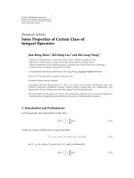
Figure 1: The single HAP with multiple-directional antennas and terrestrial point-to-point links.
for example, for an HDTV specialist user discussed above.
Normally, specialist users are served by satellites, which due
to link budget constraints will supply links with data rates
of much less than 1 Gbps. Moreover, the users themselves
operate outside broadcast equipment, vans, and so forth,
which require a steerable dish to provide the links. Given
these disadvantages, high-altitude platforms (HAPs) provide
a practical alternative with the ability to provide both high
data rate signals, due to the 69 dB link budget advantage
compared to GEO satellites and the necessary flexibility to
immediately respond to the demands from the users, while
serving a wide area of coverage.
This paper is composed of three sections: we will discuss
the system scenario in the following section which will
discuss the three schemes: the short step size scheme, the
half distance step size scheme, and the beam switch scheme;
system performance will be deliberated after each scheme; we
also draw conclusions at the end of this paper.
2. SYSTEM SCENARIO
The International Telecommunications Union (ITU) has
provided a regulatory framework for HAPs to provide 3G
services at 2 GHz and also in the millimeter-wave bands
around 28/31 and 47/48 GHz [3–7]. Since high-altitude
platforms will operate in the stratosphere, it gives them a
significant link budget advantage compared with satellites,
and a wider coverage area than terrestrial systems. In our
scenario, the HAP station and terrestrial stations will share
a same frequency band of 28 GHz. We examine the feasibility
of such an approach because in this band, HAPs will have
to share this band with terrestrial systems. Moreover, the
highly directional antenna characteristics of both terrestrial
users and HAP specialist users should mean that coexistence
is feasible, providing access to the spectrum is appropriately
controlled.
Thus, the scenario consists of an HAP capable of deliv-
ering multiple spot beams point-to-point links alongside
multiple terrestrial point-to-point links located inside the
HAP service area. To provide the greatest flexibility, we
examine the situation, where the HAP station is located away
from the center of the service area, which is 60–300 km in
diameter. The terrestrial stations are randomly located inside
the service area as shown in Figure 1. For the HAP station,
we consider multiple-directional aperture antennas (we use
20 antennas in this scenario) operated from a single aircraft,
pointing at random points of interest within the service area.
For the point-to-point terrestrial link, the two-terrestrial
stations point directly to each other using highly-directional
antennas, as point-to-point communications links. These
links share the same frequency as the HAP. HAP users are
assumed to point their directional antennas directly toward
the HAP.
Unlike the papers that have considered the potential
coverage area served, we are more concerned with the
interference to the ground user from both the terrestrial
stations and other antennas on the HAP which serve other
users. The interference due to coexistence of both systems
using the same frequency band is evaluated in order to
determine the mutual impact on the systems. To evaluate
both impacts, we first have to calculate two important system
parameters, the carrier to noise ratio (CNR) and the carrier
to interference plus noise ratio (CINR). The performance of
this scheme relies on the fact that the CNR and CINR can be
Z. Peng and D. Grace 3
evaluated at different points on the service area. The CINR
of both HAP and terrestrial test users can be calculated as in
[8–10]:
CINR
=
C
N
F
+ I
=
P
Hm
A
Hm
(ϕ
m
)A
U
(θ
m
)(λ/4πd
m
)
2
N
F
+
N
j
=1
P
Hi−j
A
Hi−j
(ϕ
j
)A
U
(θ
j
)(λ/4πd
m
)
2
,
(1)
while the CNR can be calculated as in [5–7]:
CNR
=
C
N
F
=
P
Hm
A
Hm
(ϕ
m
)A
U
(θ
m
)(λ/4πd
m
)
2
N
F
,(2)
where N
F
is the thermal noise floor. P
Hm
and P
Hi
are the
transmit power from one antenna beam of the HAP, and
jth interfering antenna beam, respectively. A
Hm
(ϕ
m
)and
A
Hi
(ϕ
i
) are the transmit gain of base station antenna, and
jth interfering HAP antennas at an angle φ
m
away from
boresight. A
U
(θ
m
)andA
U
(θ
i
) are the receive gain of the
user antenna for the main, and jth interfering at an angle
θ
m
away from its boresight. λ/4πd
m
is the path loss from
the main antenna beam, and the jth interfering antenna
beam. λ is the wavelength, and d
m
is the distance between the
HAP station and the ground user. Techniques for producing
elliptic beam antennas for optimizing geographical coverage
are also discussed in [11, 12].
2.1. Antenna gain factor
The HAP and user antenna discussed in Section 2 can be
described in terms of the main lobe and sidelobes, producing
the following equations, respectively, [4–7],
A
H
(ϕ) = G
T
(max[cos
n
H
(ϕ), s
f
]),
A
U
(θ) = G
R
(max[cos
n
U
(θ), s
f
]),
(3)
where G
T
is the boresight gain of the HAP, G
R
is the boresight
gain of the user antenna, and s
f
is the main lobe associated
with the sidelobe. G
= η·(π·k/α)
2
,whereη is the antenna
efficiency, k is a factor that depends on the shape of the
reflector and the method of illumination, α is the half power
beamwidth. n
H
and n
U
control the rate of the main beam
power roll-off of the HAP antenna and the user antenna,
respectively. We adopt a circularly symmetric beam in order
to simplify the calculation and assume that it can point in
any direction to serve users in the service area. The transmit
power from all users/antenna beams of HAP is assumed to
be identical.
2.2. Antenna sidelobe analysis
In our scenario, we do not apply a flat sidelobe model, for
example,
−30 dB as used in other papers since the absolute
sidelobe level is more important for this case due to the high
gain of the main lobe. Here, we use the model suggested
by ITU-R to more accuracy in the region of the main lobe
and for sidelobe [8]. Thus, the possible pattern commencing
0
10
20
30
40
Gain relative to G
m
(dB)
0 2 4 6 8 101214161820
Off-axis angle (degrees)
Sidelobe model of the HAP antenna
−3dB
A
BCD
Figure 2: Radiation pattern envelope function.
at the boresight of the main lobe can be divided into five
regions. These are illustrated in Figure 2.
The four regions below the
−3 dB point can be described
as follows [11]:
(A)
G(Ψ)
= G
m
−3
Ψ
Ψ
0
2
(4)
for Ψ
0
≤ Ψ ≤ 2.58Ψ
0
,
(B)
G(Ψ)
= G
m
+ L
s
(5)
for 2.58Ψ
0
≤ Ψ ≤ 6.32Ψ
0
,
(C)
G(Ψ)
= G
m
+ L
s
+20−20 log
Ψ
Ψ
0
(6)
for 6.32Ψ
0
≤ Ψ ≤ Ψ
1
,
(D)
G(Ψ)
= 0(7)
for Ψ
1
≤ Ψ.
Where G(Ψ) represents the gain at the angle (Ψ)from
the boresight (dBi); G
m
is the maximum gain in the main
lobe (dBi); Ψ
0
is the one-half 3 dB beamwidth in the plane
of interest (3 dB below G
m
) (degrees); Ψ
1
is the value of (Ψ)
when G(Ψ)in(6)isequalto0dBi;L
s
is the required near-
in-sidelobe level (dB) relative to the peak gain. This model is
not difficult to apply when operating with a circular beam.
2.3. System parameters
With this scenario, we consider the effect of the antenna
beamwidth on performance by setting the beamwidth of
both HAP and terrestrial station antennas to 5 degrees. The
important system parameters for the HAP, terrestrial station,
and test users are shown in Ta bl e 1 .
3. LOCATION OF PEAK RECEIVED
POWER CALCULATION
Figure 3 shows the relationship between the peak received
power location and the aiming point of the HAP antenna.
Given that these highly-directional antennas on the HAP
are not likely to point toward the subplatform point, the
4 EURASIP Journal on Wireless Communications and Networking
HAP
station
HAP coverage area
S
β
X
P
A
P
Aiming point
(A
px
, A
py
)
Peak power point
(P
x
, P
y
) Sub-platform point
Figure 3: Peak receiving point and aiming point from different directional antennas of a single HAP.
Table 1: System parameters.
Parameter HAP base station Terrestrial point-to-point terminal Specialist user
Coverage radius 150 km N/A N/A
Transmitter height 17 km 10 m 10 m
Antenna gain 31.4 dB 31.4 dB 45.4 dB
Roll off rate 727.9 727.9 18204
Antenna beamwidth 5 degrees 5 degrees 1 degree
Frequency 28 GHz
Side lobe level specified
Noise power
−103.8 dBW
peak received power point deviates from the aiming point
due to the path loss gradient behavior between the SPP
and the POI. This deviation is a very important factor
that concerns us because specialist users will require good
received power performance. The more the boresight of the
antenna deviates from the perpendicular line, the further the
peak received power point deviates from the aiming point.
Given this mutual interaction between the peak received
power point and the aiming point of antenna, we can
calculate the optimum aiming point of a directional antenna
from the HAP by specifying the peak received power location
first as required by the individual specialist ground users.
More information in detail will be given to show how the
peak received power location and/or aiming points can be
calculated.
In our scenario, the HAP is assumed not to be at the
center of the service area, so it means the HAP spacing radius,
defined as the distance from the center of the service area
to the subplatform point (SPP) is nonzero (here assumed to
equal 10 km). The peak received power location will be on
the same line with the aiming point, so we can use the same
coordinate ratio (e.g., assuming a set of x coordinates, then
x1/x2
= x3/x4) to calculate the unknown parameter (aiming
point or peak CNR point).
Changing the beamwidth of the HAP antenna will cause
the location of the peak received power also to move, as can
a change in the spacing radius. It is possible to derive the
location of the peak received power from the HAP taking
into account spacing radius, antenna roll-off, and pointing
offset. Assuming that the center of the service area and the
antenna aiming point are along the X-axis, the location of the
peak received power point will also move along the X-axis. To
calculate the location of peak received power as a function
of HAP location and HAP antenna pointing location, we
can differentiate the carrier part of (1)withrespecttouser
location and set it equal to zero. Equation (1)isdifferentiated
as [6]
d(Carrier)
dx
=
d[P
Hm
A
Hm
(ϕ
m
)A
U
(θ
m
)(λ/4πd
m
)
2
]
dx
= 0.
(8)
Only cos
n
H
(φ)andd
2
m
are related to the user location, so we
may write [6] the following:
d(Carrier)
dx
=
d[cos
n
H
(ϕ)(1/d
m
)
2
]
dx
= 0, (9)
Z. Peng and D. Grace 5
where [6]
cos(ϕ)
=
[(S −X)
2
+ H
2
]+[(S −P)
2
+ H
2
] −(X − P)
2
2
(S −X)
2
+ H
2
·
(S −P)
2
+ H
2
,
(10)
d
m
=
(S −X)
2
+ H
2
, (11)
where P is the distance between antenna aiming point and
the center of the service area, X is the distance between peak
received power point and the center of the service area, S
is the HAP spacing radius, and H is the height of the HAP.
Finally, the following equation is derived [6]:
2(P
−S)X
2
+[4S(S −P)+H
2
(n
H
+2)]X
−2S(S
2
+ H
2
−S·P) −n
H
·H
2
·P = 0.
(12)
This quadratic equation (1)canbesolvedasafunctionofthe
above parameters to yield the location of the peak received
power on the axis as follows [6]:
X
=
−
B ±
√
B
2
−4AC
2A
, (13)
where
A
= 2(P − S),
B
= 4S(S − P)+H
2
(n
H
+2),
C
=−2S(S
2
+ H
2
−S·P) −n
H
·H
2
·P.
(14)
Now, we can generalize the result for the required aiming
point (A
px
, A
py
) on the service area in order for the peak
received power to be at point (p
x
, p
y
).
X the ground distance between the peak received power
point and the center of the service area can be derived from
(10), (12), (13), and
X
=
p
X
−S
cos β
−S, (15)
where
β
= arctan
p
Y
p
X
−S
. (16)
Thus, we have
P
=
2SX
2
−4S
2
X − H
2
(n
H
+2)·X +2S
3
−2SH
2
2X
2
−4SX − 2S
2
−n
H
·H
2
, (17)
where (A
px
, A
py
) is the location of the aiming point. This
calculation is based on the proof [6] that the peak received
power is exactly on the line between the antenna aiming
point and the HAP subplatform point. As we know the
method to calculate the peak received power point, we
could alternatively derive the location of aiming point of the
antenna by using a given peak received power point. The
equations are shown as
A
px
= (P − S)cosβ + S,
A
py
= (P − S)sinβ.
(18)
Start
Point the antenna beam at the point of interest
Calculate the distance between
POI and peak CINR for each beam
Move the aiming point toward the POI by a certain
step size related to the coefficient
Move the aiming point based on a certain number
of iteration which will pass the minimum mean
distance value point according to the mean
distance variation graph
Record the minimum mean distance value based
on the mean distance variation graph
Use the step which has the minimum
value as the aiming point allocation
End
Figure 4: Flowchart of small step size scheme.
Given this mutual relationship between the two points, we
can also extend this analysis to additionally calculate the
location of the peak received power point, given a specific
aiming point.
4. CONTROLLING CINR BEHAVIOR
The HAP station in this scenario is aimed to serve the
specialist users by using several directional antennas identical
in number to the specialist users. Each antenna will directly
point at a certain location which can give the respective
user the peak CNR that we call the point of interest (POI).
However, as the number of beams increases, the peak CINR
point of the antenna will not coincide with the POI due to
the interference from other antenna beams and the terrestrial
systems. The purpose of the schemes developed here is to
move the peak CINR to the point of interest, while coping
with the mutual interaction caused by the interference.
4.1. Scheme I: small step size scheme
From an antenna beam perspective, the aiming point deter-
mines the level of the CINR, so that moving the aiming point
is the way to modify the location of the peak CINR. However,
applying the scheme by modifying only the pointing of
one antenna will impact on the other CINR levels seen by
other users inside the service area. In order to mitigate such
a problem, we apply the scheme to every HAP antenna
beam simultaneously with the aim of reducing the mutual
interference.
As the distance between the point of interest and the
peak CINR point of each antenna beam is different, we are
unable to ensure that peak CINR and POI coincide after
the iteration, so instead we apply the algorithm repeatedly.
Concerned with the distance between peak CINR and POI
6 EURASIP Journal on Wireless Communications and Networking
HAP
station
HAP coverage area
Aiming point 2
−−−→
r
Ai+1
Aiming point 1
−→
r
Ai
Peak power point 2
−−−→
r
Pi+1
Peak power point 1
−→
r
Pi
Point of interest
Sub-platform point
Figure 5: The small step scheme description.
0
5
10
15
20
Mean distance (km)
0 20 40 60 80 100 120
Iteration
The mean distance with different coefficient
0.1
0.15
0.05
0.025
0.01
Figure 6: The mean distance between peak CINR and POI with
different coefficients in a small step scheme.
points, we move each aiming point of the beam in the
same ratio. We can see how the small step scheme works in
Figure 4.
The small step size scheme moves the aiming point based
on a very short distance each time according to the flowchart
shown in Figure 4. The step size can be specified in terms of
the distance between peak CINR point and the POI with the
aim of iteratively moving the CINR point closer to the POIs.
To make it clear, if the initial distance between the two points
is 10 km , with a ratio δ of 0.05, then the aiming point will
move iteratively along the line joining the two by 0.5 km each
time.
As shown in Figure 5, the subplatform point, POI, and
the aiming point are in a straight line. We also assume that
the interference at the peak CINR point is much lower than
the signal in that region, which means that the peak CINR
point will lie close to the same line. According to the figure,
the peak CINR point is always at the far side from the
subplatform to the POI, so that in order to move the peak
CINR point closer to the POI, we should move the aiming
point toward to the SPP with each step. We also assume the
peak CINR point is close to the straight line containing the
aiming point, POI, and SPP.
This scheme can be expressed by the following equation:
−−→
r
Ai+1
= (1 + δ)
−→
r
Ai
−δ
−→
r
Pi
, (19)
where
−−→
r
Ai+1
,
−→
r
Ai
,
−→
r
Pi
represent the position vector for the
different points in the x, y plane, where
−−→
r
Ai+1
represents the
vector with the symbol.
We repeat the same process at each step (i) which means
the generated location in one step will be the condition of
next step (i + 1) to calculate the new location of the aiming
point.
The short step size scheme will not deliver the optimum
aiming point after a single stage, so it needs a number
of iterations to reach the minimum value. In general, the
shorter the step size, the more iterations that are needed
to reach the optimum point. However, the scheme moves
in a single direction toward the SPP, so it will continue to
move the peak CINR beyond the POI after it reaches the
minimum point. Therefore, we store the outcome of value
after each iteration in order to select the optimum iteration
value to minimize the distance between the peak CINR and
POI. We assume the optimum mean number of iterations
occurs when the distance between the peak CINR and POI is
a minimum that is,
d
min
= min
mean
−−−→
r
POI j
−
−−−−−→
r
PCINR j
, (20)
where j is the set of beams sharing the same channel.
Figure 6 illustrates the variation of the mean distance
value between the POI and peak CINR points with five
different coefficients and different iterations from the same
antenna beam allocation. This figure shows that the higher
value coefficient case requires fewer iterations to reach the
mean minimum distance which has the advantage of saving
time to finish the antenna positioning. However, the mean
minimum distance from the higher value coefficient case
tends to be less accurate than the lower ones since it may miss
Z. Peng and D. Grace 7
−150
−100
−50
0
50
100
150
Distance (km)
−150 −100 −50 0 50 100 150
Distance (km)
Max. CINR for configuration of single HAPs point
with the terrestrial systems
(a)
−150
−100
−50
0
50
100
150
Distance (km)
−150 −100 −50 0 50 100 150
Distance (km)
Max. CINR for configuration of single HAPs point
with the terrestrial systems
(b)
Figure 7: (a) Initial CINR contour plot of single HAP with multiple antenna beams with terrestrial systems. (b) Final CINR contour plot of
single HAP with multiple antenna beams with terrestrial systems after applying Scheme I.
0
20
40
60
Mean distance (km)
12345678910
Iteration
The mean distance/worst case/best case with
different random points sets
6.8
Mean worst case
Mean best case
Mean average distance
Figure 8: The mean distance/best case/worst case with different
random points sets in small step size scheme.
0
0.5
1
Probability distribution
0 102030405060708090
Distance (km)
CDF of mean distance/worst case/best case
from ten different cases
0.6
0.88
Wors t c as e
Best case
Mean distance
Figure 9: The CDF of mean distance/best case/worst case with
different random points sets in the small step size scheme.
the minimum point because of the longer step size each time.
It clearly illustrates the tradeoff between pointing accuracy
and convergence time.
To assess performance, we look at the special effects of the
scheme using a contour plot. These are shown in Figure 7.
The green circles represent the peak CINR points, red
diamonds represent the POIs, blue circles represent the
terrestrial stations, yellow circles specify the aiming points,
and the pink circle represents the SPP. As shown in Figure 7,
the 0.05 ratio coefficient has been chosen to operate the
simulation. The first figure is the initial version of CINR
contour and the second one is the modified version, where
the positions have been optimized to deliver the best mean
CINR at the POIs. Here, the optimum point is reached
after 40 iterations. As shown in the figure, most pairs of
the peak CINR points and POIs in the first figure initially
do not coincide with each other, particularly well outside
50 km radius range. However, after applying the small step
size scheme, the pairs of peak CINR point and POI within
50 km coincide even better, and those outside the 50 km
range shorten a considerable distance that can be certified
in the above figures.
Figure 8 illustrates the mean distance variation between
POI and peak CINR for up to 10 iterations. The mean
distance drops down smoothly at the beginning, after
reaching the minimum point (after 9 iterations) it increases
as the peak CINR and POI start to diverge. The minimum
value of the mean average distance is 6.8 km according to
Figure 8.
Figure 9 shows the CDFs of best, mean, and worst case
distances after 20 iterations. It illustrates that 60% of the
mean distance cases are within the range of 10 km. For the
worst cases, 88% of them are within 50 km. Note that a
50 km distance does not necessarily mean that the CINR is
inadequate at the POI, just that it is not a maximum. In any
8 EURASIP Journal on Wireless Communications and Networking
Start
Point the antenna beam at the point of interest
Calculate the distance between
POI and peak CINR for each beam
Move the aiming point toward the POI by half
distance of peak CINR point and SPP
If the new peak
CINR point is at the far side of the POI
and the SPP
Move the aiming point toward the POI by half
distance of new peak CINR point and previous
peak CINR point
If the current iteration
number exceed the max iteration number
that designed
Use the step which has the minimum value
as the aiming point allocation
Move the aiming point
toward the POI by half
distance of peak CINR
point and the initial peak
CINR point
Ye s
Ye s
No
No
End
Figure 10: The flowchart of the half distance step side scheme.
case, the schemes discussed later show how the peak CINR
can be moved closer to the POI.
4.2. Scheme II: half distance step size scheme
The previous scheme moved the aiming point by a short
fixed step each iteration and always moved in the same
direction toward the SPP, which means that it will deviate
from the POI after reaching it, making it difficult to predict
the optimum number of iterations. The half distance step
size scheme is a creative method to move the peak CINR
point to coincide with the POI. This is based on a basic
binary search technique. The movement operates similar to
the previous scheme, since it still concentrates on moving
the aiming point along the line joining the subplatform
(SPP) and the POI. However, unlike the short step scheme,
we move the aiming point depending on whether the peak
CINR point with the new allocation is between the SPP and
the POI or instead outside these two points. The aiming
point is iteratively moved each step by half the distance
separating the initial or last previous peak CINR point and
new peak CINR point, either toward or away from the SPP,
depending on the location of the previous position relative
to the POI. The mean distance of all peak CINR points
and POIs are evaluated each iteration and the process stops
after the minimum point has been reached or the maximum
number of iterations has occurred. We can see how the half
distance scheme works in Figure 10.
The direction of movement is determined by the mutual
position of new peak CINR point and POI, however, it always
moves toward the POI. To make it clear, we can see how the
aiming point changes in Figure 11.
D
1
is defined as the distance between the initial peak
CINR point and SPP. Each step, the new location changes to
Z. Peng and D. Grace 9
D
1
/2
D
2
/2
D
3
/2
1st 3rd
Final
2nd
D
1
D
2
D
3
HAP
station
Peak CINR point
Aiming point
Point of interest
Subplatform point
Figure 11: The half distance scheme description.
the one between the new peak CINR point and subplatform
point (if the new peak CINR point’s location is between the
POI and SPP) or the one between the initial peak CINR point
and new peak CINR point (if the new peak one is between
the initial peak CINR point and POI). This scheme ends
when the mean distance between peak CINR and POI of all
the beams of the previous iteration is less than the current
iteration. This scheme is better than Scheme I since it will
converge more quickly toward the coordinates of the aiming
point.
The scheme can be described by the following equations:
When
−π/2 < arccos(
−−→
POI·
−→
a
s
/|
−−→
POI||
−→
a
s
|) ≤ π/2,
−−→
r
i+1
=
⎧
⎪
⎪
⎪
⎪
⎪
⎪
⎨
⎪
⎪
⎪
⎪
⎪
⎪
⎩
−−−→
PC
i−1
+
−→
r
i
2
,
−
π
2
<arccos
−−→
POI·
−−−−→
PCINR
|
−−→
POI·
−−−−→
PCINR|
≤
π
2
,
−−→
PC
i
+
−→
r
i
2
,
π
2
<arccos
−−→
POI·
−−−−→
PCINR
|
−−→
POI·
−−−−→
PCINR|
≤
3π
2
,
(21)
when π/2 < arccos(
−−→
POI·
−→
a
s
/|
−−→
POI||
−→
a
s
|) ≤ 3π/2,
−−→
r
i+1
=
⎧
⎪
⎪
⎪
⎪
⎪
⎪
⎨
⎪
⎪
⎪
⎪
⎪
⎪
⎩
−−−→
PC
i−1
+
−→
r
i
2
,
π
2
<arccos
−−→
POI·
−−−−→
PCINR
|
−−→
POI·
−−−−→
PCINR|
≤
3π
2
,
−−→
PC
i
+
−→
r
i
2
,
−
π
2
<arccos
−−→
POI·
−−−−→
PCINR
|
−−→
POI·
−−−−→
PCINR|
≤
π
2
,
(22)
where
→
r
is the vector of the aiming point,
→
a
s
is the vector
of SPP,
−−→
POI is the vector of POI,
−−→
PC
i
is the vector of the peak
carrier value, and
−−−−→
PCINR is the vector of the peak CINR used
in the calculation.
0
4.1
20
40
60
80
Mean distance (km)
0 5 10 15 20 25
Iteration
The mean distance/worst case/best case with
different random points sets
Mean worst case
Mean best case
Mean average distance
Figure 12: The mean distance/best case/worst case with different
random points sets in half distance scheme.
In order to compare the mean distance variation with
the short step size scheme, this section will show the mean
value, worst case, and best case in the simulation process.
Figure 12 illustrates the mean distance variation for up to 20
iterations. All the first steps have a very high value due to
the initial moving distance being the longest. After a series
of fluctuating adjustments, the value becomes stable and
appears as the best situation in the process. All the best cases
beyond 4 iterations in Figure 12 are equal to zero which
means at least one POI receives the highest CINR value, and
all the worst cases in Figure 12 distribute between 30 km and
40 km due to the interference from the terrestrial stations
and other antenna beams. The minimum value of the mean
average distance is 4.1 km which is 2.7 km less than Scheme
I. The results from both schemes are based on 100 sets of
random points.
Figure 13 shows the CDFs of best, mean, and worst case
distances after 20 iterations. It shows that 75% of the mean
distance cases are within 10 km on average, with 82% of the
10 EURASIP Journal on Wireless Communications and Networking
0
0.5
1
Probability distribution
0 10203040 5060708090
Distance (km)
CDF of mean distance/worst case/best case
from ten different cases
0.75
0.82
Wors t c as e
Best case
Mean distance
Figure 13: The CDF of mean distance/best case/worst case with
different random points sets in half distance scheme.
0
0.2
0.4
0.51
0.6
0.72
0.8
0.92
Probability distribution
0 5 10 15 20 25 30
Distance (km)
CDF of mean distance from 64QAM/16QAM/QPSK
threshold cases
64QAM
16QAM
QPSK
Figure 14: CDF plot of mean distance, worst case, and best case
from 64 QAM, 16 QAM, and QPSK modulation scheme.
worst cases being within 50 km. Given the worst case is with a
long physical distance, the CINR values at the POIs that they
serve are still satisfied under the user’s demands. Comparing
the mean distance results shows that 75% are below 10 km
for Scheme II with 60% for Scheme I. Furthermore, Scheme
II normally requires fewer iterations to achieve the same or
better minimum mean distance values.
4.3. Scheme III: beam switch off
In this section, we modify Scheme II introduced in the
previous section by switching off some of the antenna
beams, where the CINR falls below a given level after a set
number of iterations, with the aim of reducing the mean
distance between peak CINR and POI. In practice, not all
the ground users need to be serviced at the same time,
and meanwhile the ground users will also require a certain
minimum CINR in order to deliver a certain level of service,
so such an approach is justified. The first part of the scheme
isidenticaltoSchemeII,anditisonlywhenthenumber
of iterations required to reach the minimum value (d
min
)is
confirmed, that the beams failing to meet a predetermined
CINR threshold at point of interest are switched off; the
CINR is reevaluated. We can see the scheme performance in
Figure 14.
We pick three different CINR threshold values to exam-
ine their mean distance, worst case, and best case perfor-
0
0.5
1
Probability
12345678910111213
Number of beams activated
Histogramofnumberofbeamsactivatedfor
QPSK/16QAM/64QAM
64QAM
16QAM
QPSK
Figure 15: Histogram of numbers of beams activated from 64
QAM, 16 QAM, and QPSK modulation scheme.
mance. The figure illustrates that the 64QAM with a 20 dB
SINR threshold always has the least distance discrepancy,
compared with 16QAM with a 16 dB SINR threshold and
QPSK with a 7.8 dB SINR threshold cases under all the three
circumstances. Using mean distance case as example, 92% of
64QAM cases are within a 10 km range, while the 16QAM
and QPSK cases have their respective 72% and 51% within
the same distance. Even the worst case 64QAM results offer
a solid performance in the 0–90 km range from the center of
coverage.
To examine how many beams are still activated after
applying the scheme with different modulation rates, we
provide a bar chart in Figure 15. The QPSK case normally
maintains 11–13 beams when it operates; the 16 QAM can
usually operate 1–5 beams, but more commonly there are 3
or 5 beams activated; the 64 QAM modulation scheme has
only 1-2 beams, but sometimes only one beam can pass the
threshold.
5. CONCLUSION
We have shown how it is possible to use directional antenna
beams on an HAP to provide gigabit link communication to
the designated specialist user over an extended service area of
300 km diameter. Furthermore, this paper presented a means
to accurately direct the peak CINR value to the location of the
user under the interference from terrestrial point-to-point
systems and other beams on the HAP. It also proposed a
technique to further improve performance by switching off
the antenna beams which fail a CINR threshold value at
the specialist user, in order to improve the CINR at other
specialist user locations. We have shown that the number of
beams which remain active on the same channel depends on
the chosen modulation level at the specialist user. Typically,
only 1 or 2 beams can operate with 64QAM, but typically,
11–13 beams remain active with QPSK. Overall, these results
indicate that HAP and terrestrial systems can coexist on the
same frequency, with the potential to offer gigabit rates to
specialist users.
Z. Peng and D. Grace 11
REFERENCES
[1] N. Geri, “Wireless HDTV-compressed or uncompressed? That
is the question,” AMIMON Ltd, November 2006.
[2]S.R.Lambert,“LegislativePolicyForumonEconomic
Development,” James W Sewall Company, 07DEC06, 2006.
[3]D.Grace,M.H.Capstick,M.Mohorcic,J.Horwath,M.B.
Pallavicini, and M. Fitch, “Integrating users into the wider
broadband network via high altitude platforms,” IEEE Wireless
Communications, vol. 12, no. 5, pp. 98–105, 2005.
[4] G. M. Djuknic, J. Freidenfelds, and Y. Okunev, “Establishing
wireless communications services via high-altitude aeronau-
tical platforms: a concept whose time has come?” IEEE
Communications Magazine, vol. 35, no. 9, pp. 128–135, 1997.
[5] Recommendation ITU-R F. 1500, “Preferred characteristics
of systems in the fixed service using high altitude platform
stations operating in the bands 47.2-47.5 GHz and 47.9-
48.2 GHz,” International Telecommunications Union, 2000.
[6] R. Miura and M. Oodo, “Wireless communications system
using stratospheric platforms: R and D program on telecom
and broadcasting system using high altitude platform sta-
tions,” Journal of the Communications Research Laboratory, vol.
48, no. 4, pp. 33–48, 2001.
[7] M. Oodo, R. Miura, T. Hori, T. Morisaki, K. Kashiki, and
M. Suzuki, “Sharing and compatibility study between fixed
service using high altitude platform stations (HAPS) and
other services in the 31/28 GHz bands,” Wireless Personal
Communications, vol. 23, no. 1, pp. 3–14, 2002.
[8] J. Thornton, D. Grace, M. H. Capstick, and T. C. Tozer,
“Optimizing an array of antennas for cellular coverage from
a high altitude platform,” IEEE Transactions on Wireless
Communications, vol. 2, no. 3, pp. 484–492, 2003.
[9]D.Grace,J.Thornton,G.Chen,G.P.White,andT.C.
Tozer, “Improving the system capacity of broadband services
using multiple high-altitude platforms,” IEEE Transactions on
Wireless Communications, vol. 4, no. 2, pp. 700–709, 2005.
[10] Z. Yang, D. Grace, and P. D. Mitchell, “Downlink performance
of WiMAX broadband from high altitude platform and
terrestrial deployments sharing a common 3.5 GHz band,”
in Proceedings of the IST Mobile Communications Summit,
Dresden, Germany, June 2005.
[11] N. Adatia, B. Watson, and S. Ghosh, “Dual polarized elliptical
beam antenna for satellite application,” in Proceedings of the
International Symposium on Antennas and Propagation Society,
vol. 19, pp. 488–491, IEEE Press, Piscataway, NJ, USA, June
1981.
[12] J M. Park, B J. Ku, Y S. Kim, and D S. Ahn, “Technol-
ogy development for wireless communications system using
stratospheric platform in Korea,” in Proceedings of the 13th
IEEE International Symposium on Personal, Indoor and Mobile
Radio Communications (PIMRC ’02), vol. 4, pp. 1577–1581,
Lisbon, Portugal, September 2002.