Báo cáo hóa học: "Research Article Monte Carlo Solutions for Blind Phase Noise Estimation" pdf

Hindawi Publishing Corporation
EURASIP Journal on Wireless Communications and Networking
Volume 2009, Article ID 296028, 11 pages
doi:10.1155/2009/296028
Research Article
Monte Carlo Solutions for Blind Phase Noise Estimation
Frederik Simoens,
1
Dieter Duyck,
1
Hakan C¸ırpan,
2
Erdal Panayırcı,
3
and Marc Moeneclaey
1
1
Department of Telecommunications and Information Processing, Faculty of Engineering, Ghent University, 9000 Gent, Belgium
2
Department of Electrical-Electronics Engineering, The University of Istanbul, Avcilar 34850, Istanbul, Turkey
3
Department of Electronics Engineering, Kadir Has University, Cibali 34083, Istanbul, Turkey
Correspondence should be addressed to Frederik Simoens,
Received 30 June 2008; Accepted 7 January 2009
Recommended by Marco Luise
This paper investigates the use of Monte Carlo sampling methods for phase noise estimation on additive white Gaussian noise
(AWGN) channels. The main contributions of the paper are (i) the development of a Monte Carlo framework for phase noise
estimation, with special attention to sequential importance sampling and Rao-Blackwellization, (ii) the interpretation of existing
Monte Carlo solutions within this generic framework, and (iii) the derivation of a novel phase noise estimator. Contrary to the
ad hoc phase noise estimators that have been proposed in the past, the estimators considered in this paper are derived from solid
probabilistic and performance-determining arguments. Computer simulations demonstrate that, on one hand, the Monte Carlo

phase noise estimators outperform the existing estimators and, on the other hand, our newly proposed solution exhibits a lower
complexity than the existing Monte Carlo solutions.
Copyright © 2009 Frederik Simoens et al. This is an open access article distributed under the Creative Commons Attribution
License, which permits unrestricted use, distribution, and reproduction in any medium, provided the original work is properly
cited.
1. Introduction
Instabilities of local oscillators are an inherent impairment of
coherent communication schemes [1, 2]. Such instabilities
give rise to a time-varying phase difference between the
oscillator at the transmitter and the receiver sides. As the
phase of the transmitted symbols conveys (part of) the
information of a coherent transmission, the carrier phase
must be known to the receiver before the recovery of the
transmitted information can take place. Estimation of the
carrierphaseishenceforthacrucialtaskofacoherent
receiver.
As long as frugality with respect to the available resources
is deemed important, this estimation process should occur
without inserting too many training or pilot symbols into
the transmitted data sequence. The presence of training
symbols in the data sequence reduces the spectral efficiency
and power efficiency of the transmission. Estimating the
carrier phase based on the unknown information carrying
data symbols is definitely more efficientinthatrespect.
Spurred by its great importance, the research on phase
noise estimation evolved into a relatively mature state nowa-
days. There already exists a myriad of estimation strategies
and most of them achieve a satisfactory performance—at
least under the specific circumstances for which they were
designed [1–5]. The existing estimators range from feed-

forward techniques assuming a piecewise constant carrier
phase over the duration of a predefined interval [1–3]to
more advanced algorithms which track the movements of
the carrier phase from symbol to symbol [4, 5]. Despite all
these ad hoc efforts, no optimal solutions—from a classical
estimation point of view—to the phase noise estimation
problem have yet been presented. Optimal estimation of the
phase noise, for example, in a maximum-likelihood or max-
imum a posteriori sense, without knowing the transmitted
information turns out to be an extremely complicated task.
The purpose of the present paper is exactly to investigate
the phase noise problem within a classical estimation context.
We will define an optimal receiver strategy and explore the
extent to which Monte Carlo methods can be used to obtain
a practical implementation of this optimal receiver. In doing
so, we will furnish a thorough overview of Monte Carlo
methods and their application to phase noise estimation. It
is only fair to point out that Monte Carlo methods have
already been considered for phase noise estimation in the
past [6, 7]. However, these solutions are limited to uncoded
2 EURASIP Journal on Wireless Communications and Networking
systems and explore only one of the possible Monte Carlo
techniques. In this paper, we will lay out a more general
Monte Carlo framework and integrate the existing estimators
within this framework. We will also present a novel estimator
and demonstrate that it bears a lower complexity than the
existing techniques.
This paper is organized as follows. Section 2 describes
the channel model. The objective of the paper and the
connection with existing phase noise estimators is outlined in

Section 3. Since it is unfair to assume that everyone working
in the field of phase noise estimation is acquainted with
Monte Carlo methods, we devote an entire and relatively
large section of this paper to the introduction of Monte
Carlo methods and sequential importance sampling in
particular (Section 4). The framework presented in Section 4
is thereafter applied to the phase noise problem for uncoded
and coded systems in Sections 5 and 6, respectively. Finally,
Section 7 provides numerical results and Section 8 wraps up
the paper.
2. Channel Model
2.1. Phase Noise Channel Model. We consider a digital com-
munication scheme, where the information is conveyed by
N complex-valued data symbols
{a
k
}
k=1, ,N
. These symbols
take on values from a predefined constellation set Ω.The
average energy of the symbols is equal to E
s
. Concerning the
channel model, we consider a discrete-time additive white
Gaussian noise channel (AWGN), susceptible to Wiener
phase noise. In order to not overcomplicate the analysis,
other receiver impairments are ignored. The received signal
samples can, therefore, be written as
r
k

= a
k
exp

jθ
k

+ n
k
,
(1)
θ
k
= θ
k−1
+ δ
k
,
(2)
for k
= 1, , N and θ
0
uniformly distributed within
[
−π, π]. The additive (thermal) noise samples {n
k
} are zero-
mean i.i.d. complex-valued and circular symmetric Gaussian
variables, with a variance of the real and imaginary part equal
to σ

2
n
. The zero-mean i.i.d. Gaussian random variables {δ
k
}
are real-valued with a variance equals to σ
2
δ
. The channel
model can equivalently be described by the following two
probability functions:
p

r
k


a
k
, θ
k

=
1
2πσ
2
n
exp

−

1
2σ
2
n


r
k
−a
k
exp

jθ
k



2

,
(3)
p

θ
k


θ
k−1


=
1
√
2πσ
δ
exp

−
1
2σ
2
δ


θ
k
−θ
k−1


2

. (4)
We assume that the receiver knows these distributions and is
able to evaluate them for different values of r
k
, a
k
, θ
k

,and
θ
k−1
.
2.2. Linearized Phase Noise Channel Model. The carrier phase
affects the received signal in a nonlinear way. As will become
apparent in the remainder of this paper, it can be useful to
linearize this model. We convert the channel model (1) into
a linear form as follows:
r
k
= a
k
exp

j

θ
k−1

exp

j

θ
k
−

θ
k−1


+ n
k
 a
k
exp

j

θ
k−1

1+j

θ
k
−

θ
k−1

+ n
k
,
(5)
where

θ
k−1
represents an initial estimate of the phase at

instant k
− 1. This approximation is valid as long as |θ
k
−

θ
k−1
|1. Hence, the linearized channel model can only be
invoked if σ
2
δ
is small, and an accurate phase estimate

θ
k−1
is
available.
3. Problem Formulation and Prior Work
In a coherent communication scheme, the receiver needs
to know the phase θ
k
at each time instant k before
detection can take place. The traditional way to acquire
this information is by estimating the carrier phase. If the
carrier phase remains constant over a relatively long period,
standard feed-forward estimation techniques can be applied.
In the presence of severe phase noise, however, other more
ingenious techniques are called upon. Before we describe our
approach in that regard, let us review some of the existing
solutions.

3.1. Prior Work. Existing phase noise estimators or trackers
have one thing in common. Their derivation does not stem
from a probabilistic analysis, but is rather driven by prag-
matic (and scenario dependent) arguments. Incidentally, the
use of feedback loops or phase-locked loops is common
practice [1].
A typical form to which these estimators can generally be
reduced is

θ
k
=

θ
k−1
+ K
k
I

r
k
a
∗
k
exp

−
j

θ

k−1

,(6)
where K
k
is a positive parameter,

θ
k
denotes the phase
estimate at instant k,and
a
k
denotes an estimate (soft or hard
decision) of a
k
, using the phase estimate from a previous time
instant and possible additional information from a decoder
(see also Section 6). Obviously, there exist other estimators
as well, for example, [8]. To our knowledge, however, their
application is limited to pilot symbols only. Estimators of
the form (6) are based on the linear model (5) and exploit
the fact that I[r
k
a
∗
k
exp(−j

θ

k−1
)] hazards an estimate of the
difference between

θ
k−1
and the true value of θ
k
. The impact
of the phase noise and the additive (thermal) noise can be
balanced by tuning the parameter K
k
. Provided the linearized
model (5) is a valid approximation, the optimal values, in a
minimum mean squared error sense, of K
k
follow from the
extended Kalman filter equations [9].
For a wide range of applications, these existing estimators
render a satisfactory performance, but they nevertheless lack
a rock-solid theoretical foundation. In the next section, we
will outline our strategy to settle this issue.
EURASIP Journal on Wireless Communications and Networking 3
3.2. Probabilistic Solution. In order to lay the foundation for
the analysis in the next two sections, let us investigate what
really determines the performance of the communication
system. For now, we will assume that the transmitted symbols
are a priori independent (and hence uncoded). The extension
to coded systems is covered separately in Section 6.Wecan
define the following on-the-fly detection rule:

a
k
= arg max
ω∈Ω
p

a
k
= ω


r
1:k

,(7)
where r
1:k
is a shorthand notation for r
1:k
.
= [r
1
, , r
k
].
The on-the-fly label stems from the fact that a decision on
a
k
can be made based on readily available information at
time instant k, that is, the received samples r

1:k
.Detectors
that exploit “future” received information are not considered
here. It is easily shown that a detector defined by (7)
minimizes the symbol error probability, again, for a receiver
that only has access to received information up to instant
k. From this, it seems that all it takes to devise an optimal
receiver is to compute and maximize p(a
k
|r
1:k
). We can
perform a marginalization with respect to the unknown
phase θ
k
and exploit the fact that the transmitted symbols
are uncorrelated. With Bayes’ rule, the probability function
canthusberewrittenas
p

a
k


r
1:k

∝

θ

k
p

a
k


r
k
, θ
k

p

θ
k


r
1:k

dθ
k
. (8)
A closed-form expression for p(a
k
|r
k
, θ
k

) follows immedi-
ately from the combination of (3) and the prior distribution
p(a
k
). Hence, the remainder of this paper will focus on the
derivation of p(θ
k
|r
1:k
) and the ensuing computation of the
integral in (8). In particular, we will investigate the use of
Monte Carlo methods for the computation of (8).
4. Monte Carlo Framework
The purpose of this section is to provide a succinct intro-
duction to Monte Carlo techniques. Section 5 addresses the
specific application to our phase noise problem.
4.1. Particle Representation. Representing a distribution by
means of samples or particles drawn from it is an appealing
alternative in case the actual distribution defies an analytical
representation. The rationale behind the particle filtering
approachisthataslongaswegenerateenoughsamplesfrom
the distribution, further processing with this distribution can
be performed using particles of the distribution rather than
the actual distribution. An example will serve to illustrate this
benefit.
Suppose that we can easily generate a number of
samples
x
(j)
, j = 1, , J

max
whose statistics are specified
by a distribution p(x). Then, we are able to approximate
expectations of the form
I
=

x
f (x)p(x)dx,(9)
by means of a particle evaluation
I
s
=
1
J
max
J
max

j=1
f


x
(j)

. (10)
It can be shown that I
s
converges to I as the number of

particles grows [10]. Hence, as long as we are able to draw
samples from p(x), it is not necessary to solve the integral
from (9) analytically. The next section elaborates the case
when sampling from p(x) is not that straightforward.
4.2. Importance Sampling. The technique outlined above
only makes sense when it is easy to draw samples from p(x).
If this is not the case, we can still proceed by using another
well-chosen distribution π(x),from which it is easy to draw
samples , and draw samples from it. Denoting these samples
again by
x
(j)
, j = 1, , J
max
, the integral from (9)canbe
approximated by
I
is
=
J
max

j=1
w
(j)
f

x
(j)


, (11)
where the so-called importance weights
w
(j)
are given by
w
(j)
∝
p


x
(j)

π

x
(j)

. (12)
These weights are normalized such that

J
max
j=1
w
(j)
= 1. The
idea is to assign different weights to the samples
x

(j)
to
compensate for the difference between the target distribution
p(x) and the importance sampling distribution π(x). Again,
it can be shown that I
is
converges to I for a large number of
samples and under mild conditions with respect to the choice
of π(x)[10].
In the remainder, we denote the particle representation
of a distribution p(x)byp(x)
↔{x
(j)
; w
(j)
}.
4.3. Sequent ial Importance Sampling. The true power of the
Monte Carlo framework gets unlocked when it is applied to
hidden Markov (or state-space) models. An observation r
k
is said to be the output of a hidden Markov process if it
complies with
r
k
∼ p

r
k



x
k

,
x
k
∼ p

x
k


x
k−1

,
(13)
where x
k
denotes the (hidden) state variable of the Markov
process and the symbol
∼ means that the right-hand side
is the probability function of the variable on the left-hand
side. Note that we do not impose any restriction about the
nature of r
k
or x
k
, these can be discrete or continuous, scalar
or vector variables.

A typical problem associated with a Markov process
involves the derivation of the a posteriori state distribution
p(x
1:k


r
1:k
) or inferences thereof. The purpose of this section
is to explain how to draw samples from p(x
1:k


r
1:k
)ina
recursive manner, the process called sequential importance
sampling (SIS).
4 EURASIP Journal on Wireless Communications and Networking
4.3.1. Derivation of the Algorithm. The first step entails the
factorization of our target distribution and manipulating it
into a recursive expression
p

x
1:k


r
1:k


∝ p

x
1:k−1


r
1:k−1

p

x
k
, r
k


x
1:k−1
, r
1:k−1

=
p

x
1:k−1



r
1:k−1
)p

x
k
, r
k


x
k−1

.
(14)
The first transition follows from Bayes’ rule and the omission
of the normalizing constant 1/p(r
k
|r
1:k−1
), whereas the
second transition exploits the Markov nature of the problem.
Now, suppose that we already have a particle representation
p(x
1:k−1
|r
1:k−1
) ↔{x
(j)
1:k

−1
; w
(j)
k
−1
}, where the samples x
(j)
1:k
−1
are drawn from a distribution π
k−1
(x
1:k−1
). From (12), we
know that the corresponding importance weights are then
given by
w
(j)
k
−1
∝ p(x
(j)
1:k
−1
|r
1:k−1
)/π
k−1
(x
(j)

1:k
−1
). The next step
is to draw, for every sample
x
(j)
1:k
−1
, a new sample x
(j)
k
from a
distribution π
k|k−1
(x
k
|x
(j)
1:k
−1
), such that x
(j)
1:k
.
= [x
(j)
1:k
−1
, x
(j)

k
]
represents a sample from
π
k

x
1:k

=
π
k−1

x
1:k−1

π
k|k−1

x
k
|x
1:k−1

. (15)
The associated importance weights follow from (14)and
(15):
w
(j)
k

=
p

x
(j)
k
, x
(j)
1:k
−1


r
1:k

π
k


x
(j)
1:k

=
p

x
(j)
1:k
−1



r
1:k−1

π
k−1


x
(j)
1:k
−1

p

x
(j)
k
, r
k



x
(j)
k
−1

π

k|k−1


x
(j)
k



x
(j)
k
−1

= 
w
(j)
k
−1
p

x
(j)
k



x
(j)
k

−1

p

r
k



x
(j)
k

π
k|k−1

x
(j)
k



x
(j)
1:k
−1

.
(16)
The choice of the importance sampling distribution

π
k|k−1
(·|·) plays an important role with respect to the
performance and stability of the algorithm. The next
section elaborates this issue furthermore. To conclude this
section, we summarize the operation of the SIS algorithm in
Algorithm 1.
4.3.2. Degeneracy of Sequential Importance Sampling. One
particularly annoying problem with SIS is that the variance
of the importance weights increases as k becomes larger [11].
This is an adverse property as it is intuitively clear that for a
fixed number of samples, the best approximation, in terms
of its ability to evaluate the expectation of a function (11),
to a distribution is obtained using equal-weight samples.
The increasing variance is so persevering that almost all
samples bear a negligible weight after a few recursions.
This implies that the distribution is represented by far less
particles than the J
max
original particles. Obviously, this does
not bode well for the accuracy of the approximation of the
distribution and the performance of ensuing algorithms.
A detriment that manifests itself especially when dealing
with high-dimensional state spaces, that is, where the state
variable x is actually a vector. Fortunately, this problem can
be resolved by taking the following measures.
(1) Start from a sample representation p(x
0
) ↔{x
(j)

0
; w
(j)
0
}
(see Section 4.2).
(2) for k
= 1toN do
(3) for j
= 1toJ
max
do
(4) Draw new sample
x
(j)
k
from π
k|k−1

x
k



x
(j)
1:k
−1

.

(5) Update the importance weights


w
(j)
k
=

w
(j)
k
−1
p


x
k, j



x
1:k−1, j

p

r
k




x
k, j

π
k|k−1


x
k, j



x
1:k−1, j

.
(6) Normalize the importance weights
w
(j)
k
=


w
(j)
k

i



w
(i)
k
.
(7) Set
x
(j)
1:k
.
=


x
(j)
k
, x
(j)
1:k
−1

.
(8)


x
(j)
1:k
; w
(j)
k


is a new sample of p

x
1:k


r
1:k

.
(9) end for
(10) end for
Algorithm 1: Sequential importance sampling.
(1) Choice of the Sampling Distribution. It is important to
carefully design the importance sampling distribution. The
distribution should generate particles or samples in the
regions of the state space corresponding to high values of the
distribution that we wish to approximate (in this case, the
posterior probability function). In this way, the correction
administered by the weights can be kept to a bare minimum.
It can be shown [11] that the variance of the weights is
minimized for
π
k|k−1

x
k



x
1:k−1

=
p

x
k


x
k−1
, r
k

. (17)
The corresponding weight update equation then becomes
w
(j)
k
= w
(j)
k
−1
p

r
k




x
(j)
k
−1

. (18)
Note that the weight update (18) does not depend on the
current sample
x
(j)
k
. This intuitively explains the optimality
of (17) since the particular choice of the samples
x
(j)
k
does
not alter the weights, and hence, does not affect (read:
increase) their variance. Unfortunately, this design measure
will only slow down the process of degeneration; it will not
bring it to a standstill. Furthermore, as will become apparent
through the remainder of this paper, it is often very difficult
to draw samples from (17). In this case, there is no alternative
than to use a suboptimal distribution. The prior importance
distribution p(x
k
| x
k−1
) forms a good alternative as it

is often easy to sample from it. The corresponding weight
update function follows from (16) and is given by p(r
k
|

x
(j)
k
).
(2) Resampling. Amoreeffective approach to avoid degen-
eracy is resampling. The idea is to remove samples with
negligible weight from the set and to include better chosen
samples (which actually contribute in a meaningful manner
to the representation of the target distribution). There are
several methods to implement this rule in practice. The
EURASIP Journal on Wireless Communications and Networking 5
prevailing method is simply to draw J
max
new and equal-
weight samples from the old distribution (defined by the
weights of the old samples). Samples associated with low
importance weights are most probably eliminated by this rule
[11, 12].
(3) Rao-Blackwellization. Lesser known, but no less inter-
esting is the Rao-Blackwellization method. The idea is that
whenever it is possible to perform some part of the recursion
analytically, it definitely pays to do so. More specifically,
it is possible to show, as an instance of the Rao-Blackwell
theorem [13, 14], that integrating out some of the state
variables in (9) analytically improves the accuracy of the

approximation (11). Moreover, it allows to sharply reduce the
number of samples used in the SIS algorithm and to mitigate
the degeneracy. In order to provide a formal outline of the
procedure, let us assume that the state variable x consists
of two parts x
.
= [y, z]. Rao-Blackwellization boils down to
converting the approximation from (11) into
I
rb
=
J
max

j=1
w
(j)
g


z
(j)

, (19)
where
g

z
(j)


.
=

y
f

z
(j)
, y

p

y | z
(j)

dy, (20)
and where p(z)
↔{z
(j)
; w
(j)
}. Again, it can be shown that I
rb
converges to I,definedin(9),foralargenumberofsamples.
Obviously, it only makes sense to rearrange (9) into (19)if
p(y
| z
(j)
) can be computed analytically, and the integration
from (20) is tractable.

In a similar vein, we can also retrieve a Rao-Blackwellized
version of the SIS algorithm [14]. It turns out that the weight
update equation is now given by
w
(j)
k
= w
(j)
k
−1
p


z
(j)
k



z
(j)
1:k
−1
, r
1:k

p

r
k




z
(j)
1:k
−1
, r
1:k−1

π
k|k−1


z
(j)
k



z
(j)
1:k
−1

, (21)
and the optimal importance sampling distribution is given
by
π
k|k−1


z
k


z
1:k−1

=
p

z
k


z
1:k−1
, r
1:k

. (22)
It is interesting to point out that, in general, the sequence z
1:k
is no longer a Markov process, neither is the observation r
k
independent from r
1:k−1
given z
1:k−1
.

5. Phase Noise Estimation for Uncoded Systems
Geared with the Monte Carlo framework from the previous
section, we are now ready to tackle our original phase noise
problem.
5.1. Joint Phase and Symbol Sampling. In a first attempt,
we cast the problem under investigation immediately into
the SIS algorithm by defining x
k
.
= [a
k
, θ
k
]. The original
state space model from (1), (2) is then a special case of the
general model from (13). Application of the SIS algorithm
immediately results in a sampled version of the a posteriori
probability function p(a
1:k
, θ
1:k
|r
1:k
).
The optimal importance sampling function is defined in
(17), and can be decomposed as follows:
π
k|k−1

x

k



x
(j)
1:k
−1

=
p

a
k
, θ
k


r
k
, a
(j)
1:k
−1
,

θ
(j)
1:k
−1


=
p

θ
k


r
k
,

θ
(j)
k
−1
, a
k

p

a
k


r
k
,

θ

(j)
k
−1

.
(23)
The decomposition above allows to produce the symbol
and phase samples in two steps. First, we draw the symbol
sample, and then for each symbol sample, we generate a
phase sample:
a
(j)
k
∼ p

a
k


r
k
,

θ
(j)
k
−1

, (24)


θ
(j)
k
∼ p

θ
k


r
k
,

θ
(j)
k
−1
, a
(j)
k

. (25)
In order to produce these samples, we need the above
functions in a closed-form expression. The first probability
function can be written as follows:
p

a
k



r
k
,

θ
(j)
k
−1

∝ p

r
k
, a
k



θ
(j)
k
−1

=
p

a
k



θ
k
p

r
k


a
k
, θ
k

p

θ
k



θ
(j)
k
−1

dθ
k
.
(26)

The exact evaluation of the right-hand side of (26)requiresa
numerical integration which is not very practical. However,
as shown in Appendix A, we can obtain the following closed-
form approximation, valid for small σ
2
δ
:
p

r
k
, a
k



θ
(j)
k
−1

∝
p

a
k

exp

−

1
2σ
2
n
+2


a
k


2
σ
2
θ


r
k
−e
j

θ
(j)
k
−1
a
k



2

.
= f
(j)
1

a
k

.
(27)
Note that p(a
k
|r
k
,

θ
(j)
k
−1
)isequalto f
(j)
1
(a
k
) up to a scaling
factor. It remains to normalize this function before samples
can be drawn.

In Appendix B, we show that the distribution from (25)
can be reduced to
p

θ
k


r
k
,

θ
(j)
k
−1
, a
(j)
k

∝
p

r
k


θ
k
, a

(j)
k

p

θ
k



θ
(j)
k
−1

∝
exp

−
1
2σ
2
u


θ
k
−θ
u



2

,
(28)
where θ
u
and σ
2
u
are given by
θ
u
=

θ
(j)
k
−1
+
σ
2
u
σ
2
n
I

r
k


a
(j)
k

∗
exp

− j

θ
(j)
k
−1

, (29)
σ
2
u
=
σ
2
n
σ
2
δ
σ
2
n
+




a
(j)
k


2
σ
2
δ
. (30)
6 EURASIP Journal on Wireless Communications and Networking
From (28), it follows that the updated samples

θ
(j)
k
are
obtained by generating Gaussian samples with mean θ
u
and
variance σ
2
u
. Finally, the associated weight update function
(18) follows immediately from (27)
p


r
k



a
(j)
1:k
−1
,

θ
(j)
1:k
−1

=
p

r
k



θ
(j)
k
−1

=


a
k
∈Ω
f
(j)
1

a
k

.
(31)
Bene fits and Drawbacks. The benefit of this algorithm is
that it renders an asymptotically optimal solution, for a
high number of particles, to the phase noise problem,
provided that the linearized channel model approximation is
accurate.
The major drawbacks are as follows.
(i) The sample space is two-dimensional. In general,
more samples are required to represent a distribution
of more than one variable. Obviously, this weighs on
the overall complexity.
(ii) In order to generate a new sample pair [
a
(j)
k
,

θ

(j)
k
],
one has to evaluate (27), (29), and (31). These
equations are relatively complicated and have to be
executed for all k, j.
(iii) Finally, the algorithm is based on the linearized
channel model and tends to be less accurate for
higher values of σ
2
δ
.
5.2. Rao-Blackwellization. To overcome the drawbacks
encountered with the previous method, we explore
the application of the Rao-Blackwellization method in
this section. We distinguish two separate approaches.
The first one is a symbol-based sampling method. This
method is not new and has already been investigated in
[6], albeit without establishing the link with the Rao-
Blackwellization framework. For completeness, we provide a
Rao-Blackwellized derivation of the algorithm in this paper.
In the second and new approach, we only draw samples
of the carrier phase. As we will demonstrate, this offers
significant computational advantages.
5.2.1. Symbol-Based Sampling. We apply the Rao-
Blackwellization method from Section 4.3.2 by setting
y
= θ
1:k
and z = a

1:k
. The optimal importance sampling
distribution is given by (22), which, for the current scenario,
breaks down to
π
k|k−1

a
k



a
(j)
1:k
−1

= p

a
k


r
1:k
, a
(j)
1:k
−1


∝
p

a
k
, r
k


r
1:k−1
, a
(j)
1:k
−1

=

θ
k
p

a
k
, r
k


θ
k


p

θ
k


r
1:k−1
, a
(j)
1:k
−1

dθ
k
.
(32)
The distribution p(θ
k
| r
1:k−1
, a
(j)
1:k
−1
)canbefoundina
recursive manner by applying a Kalman filter to the state
space model of (5), (2),whichisequivalenttoanextended
Kalman filter applied to (1), (2). In Kalman parlance, the

requested distribution corresponds to the prediction step
of the Kalman filter. For every symbol sequence
a
(j)
1:k
−1
,we
should run a Kalman filter to keep track of the carrier phase
distribution. This means that we should run J
max
Kalman
filters in parallel with the SIS algorithm. Denoting the mean
and variance of the carrier phase distribution by μ
(j)
k
|k−1
and
σ
(j)2
k
|k−1
, respectively, the integral from (32) can be evaluated
analytically as follows:
π
k|k−1

a
k




a
(j)
1:k
−1

∝
p(a
k
)exp

−
1
2σ
(j)2
s


r
k
−a
k
e
jμ
(j)
k
|k−1


2


.
= f
(j)
2

a
k

,
(33)
where σ
(j)2
s
.
= σ
2
n
+σ
(j)2
k
|k−1
. The weight update function follows
from (21) and is given by
p

r
k



r
1:k−1
, a
(j)
1:k
−1

=

a
k
p

a
k
, r
k


r
1:k−1
, a
(j)
1:k
−1

=

a
k

∈Ω
f
(j)
2

a
k

.
(34)
Denote the mean and variance of the carrier variable at
instant k conditioned on the observations up to instant l by
μ
k|l
and σ
2
k
|l
, as follows: This succinct derivation captures the
main idea and furnishes the key equations of the symbol-
based sampling approach.
Bene fits and Drawbacks. The main benefit of this approach
is the reduction of the sample space to one dimension. By
running a Kalman filter in parallel with the particle filter,
the posterior distribution of the carrier phase can be tracked
analytically.
However, the following two drawbacks remain.
(i) The algorithm still relies on the linearized channel
model and suffers from the disadvantages mentioned
in Section 5.1.

(ii) The computational complexity remains high due to
the required evaluation of (33), (34), and the Kalman
filter evaluation.
5.2.2. Phase-Based Sampling. In this second method, sam-
ples are drawn of the carrier phase rather than of the data
symbols. We will distinguish two different approaches within
this method. In the first approach, we use the optimal
importance sampling distribution, whereas in the second
approach, an alternative distribution is explored. We will
show that the suboptimal sampling method results in a lower
overall complexity.
EURASIP Journal on Wireless Communications and Networking 7
(a) Optimal Distr ibution. The optimal importance sampling
distribution for the present case follows again from (22)as
follows:
π
k|k−1

θ
k



θ
(j)
1:k
−1

=
p


θ
k


r
1:k
,

θ
(j)
1:k
−1

=
p

θ
k


r
k
,

θ
(j)
k
−1


=

a
k
∈Ω
p

θ
k


r
k
,

θ
(j)
k
−1
, a
k

p

a
k


r
k

,

θ
(j)
k
−1

.
(35)
The second transition follows from the fact that u
k
.
= [r
k
, θ
k
]
is a Markov process, provided that the transmitted symbols
are independent. The first distribution in the last line has
already been derived in Section 5.1. We can simply reuse the
result obtained there if we replace
a
(j)
k
by a
k
in (28). The
second factor in (35) is also known and given by (26). Hence,
as it turns out, π
k|k−1

(θ
k
|

θ
(j)
1:k
−1
) is a mixture of Gaussian
distributions. Sampling from this, a distribution is very
simple. First, draw a sample
a
(j)
k
from p(a
k
|r
k
,

θ
(j)
k
−1
). Then,
draw a phase sample from p(θ
k
|r
k
,


θ
(j)
k
−1
, a
(j)
k
). The weight
update equation is again given by (31).
This approach is almost identical to the approach from
Section 5.1.Theonlydifference is that the samples of the data
symbols are not stored. Hence, this method will not mitigate
the inconveniences of the earlier described methods. Note
that this approach has also been investigated in [7].
(b) Prior Distribution. By carefully selecting the importance
sampling distribution, however, we can obtain a significant
saving in the overall complexity. In this paragraph, we
explore the prior distribution of the phase (at instant k
given phase samples up to k
− 1) as a candidate sampling
distribution:
π
k|k−1

x
k




x
(j)
1:k
−1

= p

θ
k



θ
(j)
1:k
−1

. (36)
Drawing samples from this distribution is very simple. All
we need is to generate Gaussian noise samples and plug them
into (2). The weight update function follows from inserting
(36) into (21) and is given by
p

r
k



θ

(j)
k

∝

a
k
∈Ω
p(a
k
)p

r
k


a
k
,

θ
(j)
k

. (37)
The functions in the right-hand side of (37) follow immedi-
ately from the channel model and are known.
Bene fits and Drawbacks. The apparent simplicity of the
latter method raises high hopes regarding the computational
complexity. The only drawback of this method is that it

does not use the optimal importance sampling distribution.
However, as we will show in Section 7, the slightly more
samples required to surmount degeneration are more than
compensated by the reduced complexity of the method.
6. Phase Noise Estimation for Coded S ystems
Let us now investigate how we can extend the algorithms
described above to a coded system. For such a coded system,
(8) is no longer valid. The a posteriori probability of a symbol
typically depends on all the entire frame of received signals.
Therefore, (8) should be replaced with
p

a
k
| r
1:k

∝

θ
1:k
p

a
k
| r
1:k
, θ
1:k


p

θ
1:k
| r
1:k

dθ
1:k
.
(38)
Straightforward application of the SIS algorithm is no
longer possible for two reasons. First, the code constraint
prohibits to draw samples from p(θ
1:k
| r
1:k
)inarecursive
manner. In particular, the evaluation of the importance
sampling and particle update equations is prohibitive in the
presence of a code constraint on the symbols. Second, the
integral in (38) cannot be evaluated using the importance
sampling technique as we have no closed-form solution for
p(a
k
| r
1:k
, θ
1:k
). The evaluation of p(a

k
| r
1:k
, θ
1:k
)requires
a complicated decoding step, which has to be executed
for every possible sample of θ
1:k
. Obviously, this becomes
impractical for a large number of samples.
Fortunately, we can extend the algorithms described
above to a coded setup by means of iterative receiver pro-
cessing. As shown in [15–19], there exists a solid framework
based on factor graph theory that dictates how the estimation
and the decoding can be decoupled in a coded setup. It can
be shown that the factor graph solution converges to the
optimal solution under mild conditions. The loops that arise
in the factor graph representation of the receiver should not
be too short. Extending the above algorithms to a coded
system boils down to replacing the prior probabilities of
the symbols p(a
k
) with the extrinsic probabilities provided
by the decoder. These extrinsic probabilities are updated by
the decoder and exchanged in an iterative fashion with the
estimator which, on its turn, updates the phase estimates.
This process repeats until convergence of the algorithm is
achieved. More details on this approach can be found in
[15, 16]. Section 7 illustrates the performance of the resulting

iterative receiver.
7. Numerical Results
We ran computer simulations to evaluate the performance
of the algorithms described above. We have adopted the
Wiener phase noise model from (1)-(2) and applied a QPSK
signaling. Unless mentioned otherwise, 50 samples were used
to represent the target distributions in the evaluation of
the various Monte Carlo-based methods. The results form
Figures 1 and 2 are for an uncoded setup, whereas Figures 3
and 4 pertain to a coded system. In this latter case, a rate-
1/2 16-state recursive convolutional code was employed, and
5 iterations between the decoder and the estimator were
performed.
The following paragraphs tender a discussion of the
obtained results.
Ambiguities. Let us begin with an uncoded configuration.
If the transmitted symbols are unknown, it is impossible to
assess the true value of the carrier phase based on the received
signal. For QPSK, for instance, the carrier phase can only be
8 EURASIP Journal on Wireless Communications and Networking
k = 10
p(θ | r
1:k
)
0
0.5
1
θ (degrees)
0 50 100 150 200 250 300 350
(a)

k = 20
p(θ | r
1:k
)
0
0.5
1
θ (degrees)
0 50 100 150 200 250 300 350
(b)
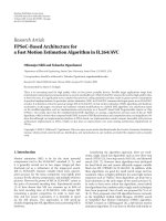
Figure 1: Histogram of p(θ|r
1:k
) ↔{

θ
(j)
; w
(j)
} obtained by the
phase-based sampling algorithm (σ
2
δ
= 5
◦
, E
b
/N
0
= 6 dB, uncoded
QPSK). The dashed line indicates the true value of θ

k
.
known up to a four-fold ambiguity. Figure 1 demonstrates
this fact. It portrays a histogram of the samples from the
distribution p(θ
k
|r
1:k
), which were obtained through the
evaluation of the phase-based sampling algorithm from
Section 5.2.2 (with the optimal sampling distribution). In
Figure 1, only the symbols at instants 11
≤ k ≤ 19 are
known to the receiver. Hence, the distribution p(θ
k
|r
1:k
)for
k
= 10 is based solely on unknown symbols. As expected,
the distribution exhibits 4 local maxima (at 90
◦
intervals).
At k
= 20, however, these ambiguities have been resolved
because of the known symbols inserted before k
= 20. This
result indicates that it is necessary to insert pilot symbols in
the data stream (at regular time instants).
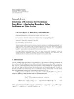
Perfor mance. Figures 2 and 3 illustrate the BER performance

of various algorithms for an uncoded and coded setups,
respectively. We considered the transmission of blocks of
400 QPSK symbols, with the periodic insertion of one pilot
symbol per 20 symbols (5% pilot overhead). The scenarios
labeled phase-based A and B correspond to the phase-based
sampling algorithm from Section 5.2.2, using the optimal
and prior importance sampling distributions, respectively.
The symbol-based algorithm corresponds to the algorithm
which was proposed in [6] and has also been described in
Section 5.2.1. These Monte Carlo approaches have also been
compared to conventional phase noise estimators. Perfor-
mance curves are included for an extended Kalman filter,
using either hard-symbol decisions, soft-symbol decisions,
or pilot symbols only (see also Section 3.1). In a coded setup,
these soft or hard symbol decisions are based on the available
posteriori probabilities of the symbols (available during the
specific iteration).
BER
10
−4
10
−3
10
−2
10
−1
10
0
E
b

/N
0
0246810
Phase-based A
Phase-based B
Symbol-based
Soft decision
Hard decision
Pilot only
Perfect phase
Figure 2: BER performance for uncoded setup (σ
2
δ
= 2
◦
,QPSK,5%
pilots).
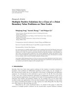
As we can observe from Figures 2 and 3, it definitely pays
to exploit information from the unknown data symbols. The
estimators that are only based on pilot symbols give rise to
a significant performance degradation. On the other hand,
there is no much difference between the performance of the
various blind estimators in the uncoded setup. This confirms
that in an uncoded setup, the conventional estimators exhibit
a satisfactory performance. In the coded configuration, how-
ever, the Monte Carlo methods outperform the conventional
methods. Apparently, these conventional ad hoc methods
fail to operate at the lower SNR-values that can be achieved
with the use of coding. We furthermore observe that the
phase-based estimators exhibit the best performance. The

reason that the symbol-based method performs not as good
is due to the fact that at high SNRs, the importance sampling
distribution is very peaky. Therefore, almost all samples
drawn from the distribution π
k|k−1
(a
k
|a
(j)
1:k
−1
)willbeequal
to each other. Hence, it takes a lot more samples to provide
an accurate representation of this latter distribution, and the
algorithm will suffer from cycle-slip-like phenomena [20].
Complexity . Finally, we will examine the computational
complexity of the different Monte Carlo-based methods.
First, we note that the complexity of each of the presented
algorithms scales linearly with the number of samples.
Hence, it suffices to determine (i) the complexity per sample
and (ii) the number of samples required to achieve a
satisfactory performance.
It is hard to assess the complexity of the algorithms in
an analytical manner. Therefore, we compared their relative
complexity per sample based on the duration of an actual
implementation on a Matlab simulation platform. Ta bl e 1
EURASIP Journal on Wireless Communications and Networking 9
BER
10
−4

10
−3
10
−2
10
−1
10
0
E
b
/N
0
012345678
Phase-based A
Phase-based B
Symbol-based
Soft decision
Hard decision
Pilot only
Perfect phase
Figure 3: BER performance for coded setup (σ
2
δ
= 2
◦
,QPSK,5%
pilots).
BER
10
−5

10
−4
10
−3
10
−2
10
−1
10
0
J
max
(number of samples)
0 1020304050607080
Phase-based A
Phase-based B
Symbol-based
Perfect phase
Figure 4: BER performance for coded setup as function of number
of samples (σ
2
δ
= 2
◦
, E
b
/N
0
= 5 dB, QPSK, 5% pilots).
displays the results. Apparently, the phase-based sampling

method with the prior importance sampling distribution
bears the lowest complexity. Based on the simplicity of this
estimator operation (see Section 5.2.2), this result does not
come as a surprise.
It remains is to compare the performance of the algo-
rithms with respect to the number of samples used in their
evaluation. Figure 4 illustrates this behavior for the coded
scenario. It turns out that the phase-based sampling methods
converge much faster to the asymptotic performance, which
is defined as the performance for J
max
→∞. Furthermore,
Table 1: Comparison of the complexity per sample of the Monte
Carlo methods (for QPSK signaling).
Method Relative complexity
Symbol-based sampling 1.26
Phase-based sampling A 1.29
Phase-based sampling B 1
the difference between the two phase-based sampling meth-
ods is negligible. Hence, based on the results from Tab le 1 ,
the phase-based sampling method with the prior importance
sampling distribution has the lowest overall complexity.
These findings advocate the use of this last method to deal
with phase noise on coded systems.
8. Conclusions
This paper explored the use of Monte Carlo methods
for phase noise estimation. Starting with a short survey
on Monte Carlo methods, several techniques were intro-
duced, such as sequential importance sampling and Rao-
Blackwellization, laying the foundation for the development

of various phase noise estimators. It turned out that there
are two feasible Monte Carlo approaches to tackle the
phase noise problem. The first one boils down to drawing
samples from the a posteriori distribution of the symbols
and updating them in a recursive manner. The carrier phase
trajectory is hereby tracked analytically. This approach has
previously been examined in [6]. The other approach entails
the sequential sampling of the a posteriori carrier phase dis-
tribution. Two different importance sampling distributions
can be used for this method. The use of the optimal sampling
distribution has been explored in [7], whereas this paper also
considers the use of the prior sampling distribution. Com-
puter simulations show that the performance complexity
tradeoff is optimized for the phase-based sampling method
with a prior importance sampling distribution.
Appendices
A. Derivation of (27)
First, we assume that the likelihood function (3)onlytakes
on significant values in the neighborhood of

θ
(j)
k
−1
. Invoking
the linearized channel model from (5), this allows to rewrite
(3) as follows:
p

r

k


a
k
, θ
k

∝
exp
⎛
⎝
−


a
k


2
2σ
2
n





r
k

a
k
e
−j

θ
(j)
k
−1
−1 − j

θ
k
−

θ
(j)
k
−1






2
⎞
⎠
=
exp


−


a
k


2
2σ
2
n
R

r
k
a
k
e
−j

θ
(j)
k
−1
−1

2
−



a
k


2
2σ
2
n
I

r
k
a
k
e
−j

θ
(j)
k
−1
−1 − j

θ
k
−

θ
(j)

k
−1


2

.
(A.1)
10 EURASIP Journal on Wireless Communications and Networking
This approximation is valid for values of θ
k
situated in the
neighborhood of

θ
(j)
k
−1
. We can now combine (A.1)and(4)
into
p

r
k


a
k
,


θ
(j)
k
−1

=

θ
k
p

r
k


a
k
, θ
k

p

θ
k



θ
(j)
k

−1

dθ
k
∝ exp

−


a
k


2
2σ
2
n
R

r
k
a
k
e
−j

θ
(j)
k
−1

−1

2
−


a
k


2
2σ
2
n
+2


a
k


2
σ
2
δ
I

r
k
a

k
e
−j

θ
(j)
k
−1
−1

2

=
exp

−
1
2

σ
2
n
+


a
k


2

σ
2
δ



r
k
−a
k
e
j

θ
(j)
k
−1


2
−


a
k


2
(
σ

2
δ
σ
2
n
)R{
r
k
a
k
e
−j

θ
(j)
k
−1
−1}
2


exp

−
1
2

σ
2
n

+


a
k


2
σ
2
δ



r
k
−a
k
e
j

θ
(j)
k
−1


2

.

(A.2)
The last approximation is valid for small σ
2
δ
. Finally, multipli-
cation with the prior symbol distribution p(a
k
)yields(27).
B. Derivation of (28)
The derivation of (28) draws on the linearized channel
model distribution (A.1) and the following straightforward
manipulations:
p

θ
k


r
k
,

θ
(j)
k
−1
, a
(j)
k


∝
p

r
k


θ
k
, a
(j)
k

p

θ
k



θ
(j)
k
−1


exp

−



a
k


2
2σ
2
n




r
k
a
k
e
−j

θ
(j)
k
−1
−1 − j

θ
k
−


θ
(j)
k
−1





2
−
1
2σ
2
δ


θ
k
−

θ
(j)
k
−1


2

∝

exp

−


a
k


2
2σ
2
n

I

r
k
a
k
e
−j

θ
(j)
k
−1

−


θ
k
−

θ
(j)
k
−1


2
−
1
2σ
2
δ

θ
k
−

θ
(j)
k
−1

2

∝
exp

⎛
⎝
−
1
2σ
2
u

θ
k
−

θ
(j)
k
−1
−


a
k


2
σ
2
u
σ
2
n

I

r
k
a
k
e
−j

θ
(j)
k
−1


2
⎞
⎠
=
exp

−
1
2σ
2
u


θ
k

−θ
u


2

,
(B.1)
where θ
u
and σ
2
u
are defined in(29)and(30), respectively.
Acknowledgments
The first author gratefully acknowledges the support from
the Research Foundation-Flanders (FWO Vlaanderen). This
work is also supported by the European Commission
in the framework of the FP7 Network of Excellence
in Wireless Communications NEWCOM++ (Contract no.
216715), the Turkish Scientific and Technical Research
Institute (TUBITAK) under Grant no. 108E054, and the
Research Fund of Istanbul University under Projects UDP-
2042/23012008, UDP-1679/10102007.
References
[1] H. Meyr, M. Moeneclaey, and S. A. Fechtel, Digital Commu-
nication Receivers: Synchronization, Channel Estimation, and
Signal Processing, vol. 2, John Wiley & Sons, New York, NY,
USA, 1997.
[2]U.MengaliandA.N.D’Andrea,Synchronization Techniques

for Digital Receivers, Plenum Press, New York, NY, USA, 1997.
[3] L. Benvenuti, L. Giugno, V. Lottici, and M. Luise, “Codeaware
carrier phase noise compensation on turbo-coded spectrally-
efficient high-order modulations,” in Proceedings of the 8th
International Workshop on Signal Processing for Space Com-
munications (SPSC ’03), vol. 1, pp. 177–184, Catania, Italy,
September 2003.
[4] N. Noels, H. Steendam, and M. Moeneclaey, “Carrier phase
tracking from turbo and LDPC coded signals affected by a
frequency offset,” IEEE Communications Letters, vol. 9, no. 10,
pp. 915–917, 2005.
[5] G. Colavolpe, A. Barbieri, and G. Caire, “Algorithms for
iterative decoding in the presence of strong phase noise,” IEEE
Journal on Selected Areas in Communications,vol.23,no.9,pp.
1748–1757, 2005.
[6]E.Panayırcı,H.C¸ ırpan, and M. Moeneclaey, “A sequential
Monte Carlo method for blind phase noise estimation and
data detection,” in Proceedings of the 13th European Signal Pro-
cessing Conference (EUSIPCO ’05), Antalya, Turkey, September
2005.
[7] P.O.Amblard,J.M.Brossier,andE.Moisan,“Phasetracking:
what do we gain from optimality? Particle filtering versus
phase-locked loops,” Signal Processing, vol. 83, no. 1, pp. 151–
167, 2003.
[8] J. Bhatti and M. Moeneclaey, “Pilot-aided carrier synchroniza-
tion using an approximate DCT-based phase noise model,” in
Proceedings of the 7th IEEE International Symposium on Signal
Processing and Information Technology (ISSPIT ’07), pp. 1143–
1148, Cairo, Egypt, December 2007.
[9] B.D.O.AndersonandJ.B.Moore,Optimal Filtering, Prentice-

Hall, Englewood Cliffs, NJ, USA, 1979.
[10] A. Doucet, S. Godsill, and C. Andrieu, “On sequential Monte
Carlo sampling methods for Bayesian filtering,” Statistics and
Computing, vol. 10, no. 3, pp. 197–208, 2000.
[11] A. Doucet, “On sequential simulation-based methods for
Bayesian filtering,” Tech. Rep. CUED/F-INFENG/TR 310,
Department of Engineering, Cambridge University, Cam-
bridge, UK, 1998.
[12] O. Capp
´
e, S. J. Godsill, and E. Moulines, “An overview of
existing methods and recent advances in sequential Monte
Carlo,” Proceedings of the IEEE, vol. 95, no. 5, pp. 899–924,
2007.
EURASIP Journal on Wireless Communications and Networking 11
[13] A. E. Gelfand and A. F. M. Smith, “Sampling-based approaches
to calculating marginal densities,” Journal of the American
Statistical Association, vol. 85, no. 410, pp. 398–409, 1990.
[14] C. Andrieu and A. Doucet, “Particle filtering for partially
observed Gaussian state space models,” Journal of the Royal
Statistical Society. Series B, vol. 64, no. 4, pp. 827–836, 2002.
[15] F. Simoens, Iterative multiple-input multiple-output communi-
cation systems, Ph.D. thesis, Ghent University, Ghent, Belgium,
2008.
[16] H. Wymeersch, Iterative Receiver Design, Cambridge Univer-
sity Press, Cambridge, UK, 2007.
[17] J. Dauwels and H A. Loeliger, “Phase estimation by message
passing,” in Proceedings of the IEEE International Conference on
Communications (ICC ’04), vol. 1, pp. 523–527, Paris, France,
June 2004.

[18] N. Wiberg, Codes and decoding on general graphs, Ph.D. thesis,
Link
¨
oping University, Link
¨
oping, Sweden, 1996.
[19] A. P. Worthen and W. E. Stark, “Unified design of iterative
receivers using factor graphs,” IEEE Transactions on Informa-
tion Theory, vol. 47, no. 2, pp. 843–849, 2001.
[20] H. Meyr and G. Ascheid, Synchronization in Digital Commu-
nications, John Wiley & Sons, New York, NY, USA, 1990.