Báo cáo hóa học: "Research Article Digital Receiver Design for Transmitted Reference Ultra-Wideband Systems" pptx

Hindawi Publishing Corporation
EURASIP Journal on Wireless Communications and Networking
Volume 2009, Article ID 315264, 17 pages
doi:10.1155/2009/315264
Research Article
Digital Receiver Design for Transmitted Reference
Ultra-Wideband Systems
Yiyin Wang, Geert Leus, and Alle-Jan van der Veen
Faculty of Electrical Engineering, Mathematics and Computer Scie nce (EEMCS), Delft University of Technology,
Mekelweg 4, 2628 CD Delft, The Netherlands
Correspondence should be addressed to Yiyin Wang,
Received 30 June 2008; Revised 6 November 2008; Accepted 1 February 2009
Recommended by Erdal Panayirci
A complete detection, channel estimation, synchronization, and equalization scheme for a transmitted reference (TR) ultra-
wideband (UWB) system is proposed in this paper. The scheme is based on a data model which admits a moderate data rate and
takes both the interframe interference (IFI) and the intersymbol interference (ISI) into consideration. Moreover, the bias caused
by the interpulse interference (IPI) in one frame is also taken into account. Based on the analysis of the stochastic properties of
the received signals, several detectors are studied and evaluated. Furthermore, a data-aided two-stage synchronization strategy
is proposed, which obtains sample-level timing in the range of one symbol at the first stage and then pursues symbol-level
synchronization by looking for the header at the second stage. Three channel estimators are derived to achieve joint channel
and timing estimates for the first stage, namely, the linear minimum mean square error (LMMSE) estimator, the least squares
(LS) estimator, and the matched filter (MF). We check the performance of different combinations of channel estimation and
equalization schemes and try to find the best combination, that is, the one providing a good tradeoff between complexity and
performance.
Copyright © 2009 Yiyin Wang et al. This is an open access article distributed under the Creative Commons Attribution License,
which permits unrestricted use, distribution, and reproduction in any medium, provided the original work is properly cited.
1. Introduction
Ultra-wideband (UWB) techniques can provide high speed,
low cost, and low complexity wireless communications with
the capability to overlay existing frequency allocations [1].
Since UWB systems employ ultrashort low duty cycle pulses

as information carriers, they suffer from stringent timing
requirements [1, 2] and complex multipath channel esti-
mation [1]. Conventional approaches require a prohibitively
high sampling rate of several GHz [3] and an intensive
multidimensional search to estimate the parameters for each
multipath echo [4].
Detection, channel estimation, and synchronization
problems are always entangled with each other. A typical
approach to address these problems is the detection-based
signal acquisition [5].Alocallygeneratedtemplateiscor-
related with the received signal, and the result is compared
to a threshold. How to generate a good template is the task
of channel estimation, whereas how to decide the threshold
is the goal of detection. Due to the multipath channel,
the complexity of channel estimation grows quickly as the
number of multipath components increases, and because of
the fine resolution of the UWB signal, the search space is
extremely large.
Recent research works on detection, channel estimation,
and synchronization methods for UWB have focused on low
sampling rate methods [6–9] or noncoherent systems, such
as transmitted reference (TR) systems [5, 10], differential
detectors (DDs) [11], and energy detectors (EDs) [9, 12].
In [6], a generalized likelihood ratio test (GLRT) for frame-
level acquisition based on symbol rate sampling is proposed,
which works with no or small interframe interference (IFI)
and no intersymbol interference (ISI). The whole training
sequence is assumed to be included in the observation
window without knowing the exact starting point. Due to
its low duty cycle, an UWB signal belongs to the class of

signals that have a finite rate of innovation [7]. Hence, it can
be sampled below the Nyquist sampling rate, and the timing
information can be estimated by standard methods. The the-
ory is developed under the simplest scenario, and extensions
2 EURASIP Journal on Wireless Communications and Networking
are currently envisioned [13]. The timing recovery algorithm
of [8] makes cross-correlations of successive symbol-long
received signals, in which the feedback controlled delay
lines are difficult to implement. In [9], the authors address
a timing estimation comparison among different types of
transceivers, such as stored-reference (SR) systems, ED
systems, and TR systems. The ED and the TR systems
belong to the class of noncoherent receivers. Although their
performances are suboptimal due to the noise contaminated
templates, they attract more and more interest because
of their simplicity. They are also more tolerant to timing
mismatches than SR systems. The algorithms in [9]are
based on the assumption that the frame-level acquisition has
already been achieved. Two-step strategies for acquisition are
described in [14, 15]. In [14], the authors use a different
search strategy in each step to speed up the procedure, which
is the bit reversal search for the first step and the linear search
for the second step. Meanwhile, the two-step procedure in
[15] finds the block which contains the signal in the first
step, and aligns with the signal at a finer resolution in the
second step. Both methods are based on the assumption
that coarse acquisition has already been achieved to limit the
search space to the range of one frame and that there are no
interferences in the signal.
From a system point of view, noncoherent receivers

are considered to be more practical since they can avoid
the difficulty of accurate synchronization and complicated
channel estimation. One main obstacle for TR systems
and DD systems is the implementation of the delay line
[16]. The longer the delay line is, the more difficult it
is to implement. For DD systems [11], the delay line is
several frames long, whereas for TR systems, it can be only
several pulses long [17], which is much shorter and easier
to implement [18]. ED systems do not need a delay line,
but suffer from multiple access interference [19], since they
can only adopt a limited number of modulation schemes,
such as on-off keying (OOK) and pulse position modulation
(PPM). A two-stage acquisition scheme for TR-UWB systems
is proposed in [5], which employs two sets of direct-sequence
(DS) code sequences to facilitate coarse timing and fine
aligning. The scheme assumes no IFI and ISI. In [20],ablind
synchronization method for TR-UWB systems executes an
MUSIC-kind of search in the signal subspace to achieve high-
resolution timing estimation. However, the complexity of the
algorithm is very high because of the matrix decomposition.
Recently, a multiuser TR-UWB system that admits not
only interpulse interference (IPI), but also IFI and ISI
was proposed in [21]. The synchronization for such a
system is at low-rate sample-level. The analog parts can run
independently without any feedback control from the digital
parts. In this paper, we develop a complete detection, channel
estimation, synchronization, and equalization scheme based
on the data model modified from [21]. Moreover, the per-
formance of different kinds of detectors is assessed. A two-
stage synchronization strategy is proposed to decouple the

search space and speed up synchronization. The property of
the circulant matrix in the data model is exploited to reduce
the computational complexity. Different combinations of
channel estimators and equalizers are evaluated to find
the one with the best tradeoff between performance and
complexity. The results confirm that the TR-UWB system
is a practical scheme that can provide moderate data rate
communications (e.g., in our simulation setup, the data rate
is 2.2 Mb/s) at a low cost.
The paper is organized as follows. In Section 2, the
data model presented in [21] is summarized and modified
to take the unknown timing into account. Further, the
statistics of the noise are derived. The detection problem is
addressed in Section 3. Channel estimation, synchronization,
and equalization are discussed in Section 4. Simulation
results are shown and assessed in Section 5. Conclusions are
drawn in
Section 6.
Notation. We use upper (lower) bold face letters to
denote matrices (column vectors). x(
·)(x[·]) represents a
continuous (discrete) time sequence. 0
m×n
(1
m×n
)isanall-
zero (all-one) matrix of size m
× n, while 0
m
(1

m
)isanall-
zero (all-one) column vector of length m. I
m
indicates an
identity matrix of size m
× m. , ⊗ and  indicate time
domain convolution, Kronecker product, and element-wise
product. (
·)
†
,(·)
T
,(·)
H
, |·|,and·
F
designate pseu-
doinverse, transposition, conjugate transposition, absolute
value, and Frobenius norm. All other notation should be self-
explanatory.
2. Asynchronous Sing le User Data Model
The asynchronous single user data model derived in the
following paragraphs uses the data model in [21] as a starting
point. We take the unknown timing into consideration and
modify the model in [21].
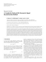
2.1. Single Frame. In a TR-UWB system [10, 21], pairs of
pulses (doublets) are transmitted in sequence as shown in
Figure 1. The first pulse in the doublet is the reference pulse,
whereas the second one is the data pulse. Since both pulses go

through the same channel, the reference pulse can be used as
a “dirty template” (noise contaminated) [8]forcorrelation
at the receiver. One frame-period T
f
holds one doublet.
Moreover, N
f
frames constitute one symbol period T
s
=
N
f
T
f
, which is carrying a symbol s
i
∈{−1, +1},spreadbya
pseudorandom code c
j
∈{−1,+1}, j = 1,2, , N
f
,whichis
repeatedly used for all symbols. The polarity of a data pulse is
modulated by the product of a frame code and a symbol. The
two pulses are separated by some delay interval D
m
,which
can be different for each frame. The delay intervals are in the
order of nanoseconds and D
m

 T
f
. The receiver employs
multiple correlation branches corresponding to different
delay intervals. To simplify the system, we use a single delay
and one correlation branch, which implies D
m
= D. Figure 1
also presents an example of the receiver structure for a single
delay D. The integrate-and-dump (I&D) integrates over an
interval of length T
sam
. As a result, one frame results in
P
= T
f
/T
sam
samples, which is assumed to be an integer.
The received one-frame signal (jth frame of ith symbol)
at the antenna output is
r(t)
= h(t − τ)+s
i
c
j
h(t −D −τ)+n(t), (1)
EURASIP Journal on Wireless Communications and Networking 3
where τ is the unknown timing offset, h(t)
= h

p
(t)  g(t)of
length T
h
with h
p
(t) the UWB physical channel and g(t) the
pulse shape resulting from all the filter and antenna effects,
and n(t) is the bandlimited additive white Gaussian noise
(AWGN) with double-sided power spectral density N
0
/2and
bandwidth B. Without loss of generality, we may assume
that the unknown timing offset τ in (1)isintherangeof
one symbol period, τ
∈ [0, T
s
), since we know the signal
is present by detection at the first step (see Section 3)and
propose to find the symbol boundary before acquiring the
package header (see Section 4). Then, τ can be decomposed
as
τ
= δ ·T
sam
+ ,(2)
where δ
=τ/T
sam
∈{0, 1, , L

s
− 1} denotes the sample-
level offset in the range of one symbol with L
s
= N
f
P,
the symbol length in terms of number of samples, and
 ∈ [0,T
sam
) presents the fractional offset. Sample-level
synchronization consists of estimating δ. The influence of

will be absorbed in the data model and becomes invisible as
we will show later.
Based on the received signal r(t), the correlation branch
of the receiver computes
x[n]
=

nT
sam
+D
(n
−1)T
sam
+D
r(t)r(t −D)dt
=


nT
sam
(n−1)T
sam

h(t −τ)+s
i
c
j
h(t −D −τ)+n(t)

×

h(t+D −τ)+s
i
c
j
h(t −τ)+n(t + D)

dt
= s
i
c
j

nT
sam
(n−1)T
sam


h
2
(t −τ)+h(t − D −τ)h(t + D − τ)

dt
+

nT
sam
(n−1)T
sam
[h(t −τ)h(t + D −τ)
+ h(t
−D − τ)h(t −τ)]dt + n
1
[n],
(3)
where
n
1
[n]
= n
0
[n]+s
i
c
j

nT
sam

(n−1)T
sam
[h(t −τ)n(t)
+ h(t
−D −τ)n(t + D)]dt
+

nT
sam
(n−1)T
sam
[h(t −τ)n(t + D)
+ h(t + D
−τ)n(t)]dt
(4)
with
n
0
[n] =

nT
sam
(n−1)T
sam
n(t)n(t + D)dt. (5)
Note that n
0
[n] is the noise autocorrelation term, and n
1
[n]

encompasses the signal-noise cross-correlation term and the
noise autocorrelation term. Their statistics will be analyzed
later. Taking
 into consideration, we can define the channel
correlation function similarly as in [21]
R(Δ, m)
=

mT
sam
(m−1)T
sam
h(t −)h(t − − Δ)dt, m = 1,2, ,
(6)
where h(t)
= 0, when t>T
h
or t<0. Therefore, the first
term in (3)canbedenotedass
i
c
j

nT
sam
(n−1)T
sam
h
2
(t − τ)dt =

s
i
c
j

nT
sam
−δT
sam
(n−1)T
sam
−δT
sam
h
2
(t − )dt = s
i
c
j
R(0, n −δ). Other terms
in x[n] can also be rewritten in a similar way, leading x[n]to
be
x[n]
=
⎧
⎪
⎪
⎪
⎪
⎪

⎪
⎪
⎪
⎪
⎨
⎪
⎪
⎪
⎪
⎪
⎪
⎪
⎪
⎪
⎩
s
i
c
j

R(0, n −δ)+R

2D, n − δ +
D
T
sam

+

R(D, n −δ)+R


D, n −δ +
D
T
sam

+ n
1
[n],
n
= δ +1,δ +2, , δ + P
h
,
n
0
[n], elsewhere,
(7)
where P
h
=T
h
/T
sam
 is the channel length in terms
of number of samples, and R(0, m) is always nonnegative.
Although R(2D, m + D/T
sam
) is always very small compared
to R(0, m),wedonotignoreittomakethemodelmore
accurate. We also take the two bias terms into account, which

are the cause of the IPI and are independent of the data
symbols and the code. Now, we can define the P
h
×1 channel
energy vector h with entries h
m
as
h
m
= R(0, m)+R

2D, m +
D
T
sam

, m = 1, , P
h
,(8)
where R(0, m)
≥ 0. Further, the P
h
× 1biasvectorb with
entries b
m
is defined as
b
m
= R(D, m)+R


2D, m +
D
T
sam

, m = 1, , P
h
. (9)
Note that these entries will change as a function of
,
although
 is not visible in the data model. As we stated
before, sample-level synchronization is limited to the estima-
tion of δ. Using (8)and(9), x[n]canberepresentedas
x[n]
=
⎧
⎨
⎩
s
i
c
j
h
n−δ
+b
n−δ
+n
1
[n], n = δ +1,δ +2, ,δ + P

h
,
n
0
[n], elsewhere.
(10)
Now we can turn to the noise analysis. A number of
papers have addressed the noise analysis for TR systems [22–
25].Thenoisepropertiesaresummarizedhere,andmore
4 EURASIP Journal on Wireless Communications and Networking
T
s
s = 1
c
1
= 1 c
2
=−1 c
3
= 1
T
f
D
···
(a)
f
s
=
1
T

sam
r(t)
D

nT
sam
+D
(n
−1)T
sam
+D
x[n]
(b)
Figure 1: The transmitted UWB signal and the receiver structure.
details can be found in Appendix A. We start by making the
assumptions that D
 1/B, T
sam
 1/B, and the time-
bandwidth product 2BT
sam
is large enough. Under these
assumptions, the noise autocorrelation term n
0
[n]canbe
assumed to be a zero mean white Gaussian random variable
with variance σ
2
0
= N

2
0
BT
sam
/2. The other noise term
n
1
[n] includes the signal-noise cross-correlation and the
noise autocorrelation, and can be interpreted as a random
disturbance of the received signal. Let us define two other
P
h
×1 channel energy vectors h

and h

with entries h

m
and
h

m
to be used in the variance of n
1
[n] as follows:
h

m
= R(0, m)+R


0, m −
D
T
sam

, m = 1, , P
h
, (11)
h

m
= R(0, m)+R

0, m +
D
T
sam

, m = 1, , P
h
. (12)
Using those definitions and under the earlier assumptions,
n
1
[n] can also be assumed to be a zero mean Gaussian ran-
dom variable with variance (N
0
/2)(h


n−δ
+ h

n−δ
+2s
i
c
j
b
n−δ
)+
σ
2
0
, n = δ +1,δ +2, , δ +P
h
. This indicates that all the noise
samples are uncorrelated with each other and have a different
variance depending on the data symbol, the frame code, the
channel correlation coefficients, and the noise level. Note that
the noise model is as complicated as the signal model.
2.2. Multiple Frames and Symbols. Now let us extend the
data model to multiple frames and symbols. We assume the
channel length P
h
is not longer than the symbol length L
s
.
A single symbol with timing offset τ will then spread over
at most three adjacent symbol periods. Define x

k
= [x[(k −
1)L
s
+1], x[(k −1)L
s
+2], , x[kL
s
]]
T
,whichisanL
s
-long
sample vector. By stacking M + N
− 1suchreceivedsample
vectors into an ML
s
×N matrix
X
=
⎡
⎢
⎢
⎢
⎢
⎢
⎢
⎢
⎣
x

k
x
k+1
x
k+N−1
x
k+1
x
k+2
x
k+N
.
.
.
.
.
.
x
k+M−1
x
k+M
x
k+M+N−2
⎤
⎥
⎥
⎥
⎥
⎥
⎥

⎥
⎦
, (13)
where N indicates the number of samples in each row of X,
and M denotes the number of sample vectors in each column
of X, we obtain the following decomposition:
X
= C
δ


I
M+2
⊗h

S + B
δ

1

MN
f
+2N
f

×N
+ N
1
, (14)
where N

1
is the noise matrix similarly defined as X,
S
=
⎡
⎢
⎢
⎢
⎢
⎢
⎢
⎢
⎣
s
k−1
s
k
s
k+N−2
s
k
s
k+1
s
k+N−1
.
.
.
.
.

.
s
k+M
s
k+M+1
s
k+M+N−1
⎤
⎥
⎥
⎥
⎥
⎥
⎥
⎥
⎦
, (15)
and the structure of the other matrices is illustrated
in Figure 2.WefirstdefineacodematrixC.Itisa
block Sylvester matrix of size (L
s
+ P
h
− P) × P
h
, whose
columns are shifted versions of the extended code vector:
[c
1
, 0

T
P
−1
, c
2
, 0
T
P
−1
, , c
N
f
, 0
T
P
−1
]
T
. The shift step is one
sample. Its structure is shown in Figure 3.ThematrixC
δ

of
size ML
s
×(MP
h
+2P
h
) is composed of M +2blockcolumns,

where δ
= (L
s
− δ

)modL
s
, δ

∈{0,1, , L
s
− 1}.Aslong
as there are more than two sample vectors (M>2) stacked in
every column of X, the nonzero parts of the block columns
will contain M
−2codematricesC. The nonzero parts of the
first and last two block columns result from splitting the code
matrix C according to δ

: C

i
(2L
s
− i +1:2L
s
,:) = C(1 : i,:)
and C

i

(1 : L
s
+ P
h
−P −i,:)= C(i +1:L
s
+ P
h
−P,:),where
A(m : n,:) refers to column m through n of A. The overlays
between frames and symbols observed in C
δ

indicate the
existence of IFI and ISI. Then we define a bias matrix B which
is of size (L
s
+ P
h
− P) × N
f
made up by shifted versions of
the bias vector b with a shift step of P samples, as shown in
Figure 3.ThematrixB
δ

of size ML
s
×(MN
f

+2N
f
) also has
M+2 block columns, the nonzero parts of which are obtained
from the bias matrix B in the same way as C
δ

. Since the bias
is independent of the data symbols and the code, it is the
same for each frame. Each column of the resulting matrix
B
δ

1
(MN
f
+2N
f
)×N
is the same and has a period of P samples.
Defining b
f
to be the P × 1 bias vector for one such period,
we have
B
δ

1

MN

f
+2N
f

×N
= 1
MN
f
×N
⊗b
f
. (16)
Note that b
f
is also a function of δ, but since it is independent
of the code, we cannot extract the timing information from
it.
Recalling the noise analysis of the previous section, the
noise matrix N
1
has zero mean and contains uncorrelated
EURASIP Journal on Wireless Communications and Networking 5
X =
C

L
s
+δ

L

s
C

δ

L
s
L
s
−δ

C
.
.
.
C
C

L
s
+δ

L
s
L
s
C

δ


C
δ

h
h
.
.
.
h
h
S +
B

L
s
+δ

B

δ

B
.
.
.
B
B

L
s

+δ

B

δ

B
δ

1
Figure 2: The data model structure of X.
P
c
N
f
−1
c
N
f
P
h
C
c
1
c
2
P
b
P
h

N
f
B
L
s
−P + P
h
Figure 3:ThestructureofthecodematrixC and the bias matrix B.
samples with different variances. The matrix Λ,which
collects the variances of each element in N
1
,is
Λ
= E

N
1
N
1

=
N
0
2


H

δ


+ H

δ


1

MN
f
+2N
f

×N
+2C
δ


I
M+2
⊗b

S

+ σ
2
0
1
ML
s
×N

,
(17)
where H

δ

and H

δ

have exactly the same structure as B
δ

,
only using h

and h

instead of b. They all have the same
periodic property, if multiplied by 1. Defining h

f
and h

f
to
be the two P
×1vectorsforonesuchperiod,weobtain
H


δ

1

MN
f
+2N
f

×N
= 1
MN
f
×N
⊗h

f
, (18)
H

δ

1

MN
f
+2N
f

×N

= 1
MN
f
×N
⊗h

f
. (19)
3. Detection
The first task of the receiver is to detect the existence
of a signal. In order to separate the detection and the
synchronization problems, we assume that the transmitted
signal starts with a training sequence and assign the first
segment of the training sequence to detection only. In this
segment, we transmit all “+1” symbols and employ all “+1”
codes. It is equivalent to sending only positive pulses for
some time. This kind of training sequence bypasses the
code and the symbol sequence synchronization. Therefore,
we do not have to consider timing issues when we handle
the detection problem. The drawback is the presence of
spectral peaks as a result of the periodicity. It can be
solved by employing a time hopping code for the frames.
We omit this in our discussion for simplicity. It is also
possible to use a signal structure other than TR signals for
detection, such as a positive pulse training with an ED.
Although the ED doubles the noise variance due to the
squaring operation, the TR system wastes half of the energy
to transmit the reference pulses. Therefore, they would have
a similar detection performance for the same signal-to-noise
ratio (SNR), that is, the ratio of the symbol energy to the

noise power spectrum density. We keep the TR structure
for detection in order to avoid additional hardware for the
receiver.
In the detection process, we assume that the first training
segment is 2M
1
symbols long, and the observation window is
6 EURASIP Journal on Wireless Communications and Networking
M
1
symbols long (M
1
L
s
= M
1
N
f
P samples equivalently). We
collect all the samples in the observation window, calculate a
test statistic, and examine whether it exceeds a threshold. If
not, we jump into the next successive observation window
of M
1
symbols. The 2M
1
-symbol-long training segment
makes sure that there will be at least one moment, at which
the M
1

-symbol-long observation window is full of training
symbols. In this way, we speed up our search procedure
by jumping M
1
symbols. Once the threshold is exceeded,
we skip the next 2M
1
symbols in order to be out of the
first segment of the training sequence and we are ready
to start the channel estimation and synchronization at the
sample-level (see Section 4). There will be situations where
the observation window only partially overlaps the signal.
However, for simplicity, we will not take these cases into
account, when we derive the test statistic. If these cases
happen and the test statistic is larger than the threshold, we
declare the existence of a signal, which is true. Otherwise, we
miss the detection and shift to the next observation window,
which is then full of training symbols giving us a second
chance to detect the signal. Therefore, we do not have to
distinguish the partially overlapped cases from the overall
included case. We will derive the test statistic using only
two hypotheses indicated below. But the evaluation of the
detection performance will take all the cases into account.
3.1. Detection Problem Statement. Since we only have to tell
whether the whole observation window contains a signal
or not, the detection problem is simplified to a binary
hypothesis test. We first define the M
1
N
f

P ×1samplevector
x = [x
T
k
, x
T
k+1
, , x
T
k+M
1
−1
]
T
with entries x[n], n = (k −
1)N
f
P+1, (k−1)N
f
P+2, ,(k+M
1
−1)N
f
P, which collects
all the samples in the observation window. The hypotheses
areasfollows.
(1) H
0
: there is only noise. Under H
0

, according to the
analysis from the previous section, x is modeled as
x
= n
0
, (20)
x
a
∼ N

0, σ
2
0
I

, (21)
where n
0
is the noise vector with entries n
0
[n], n =
(k − 1)N
f
P +1,(k − 1)N
f
P +2, ,(k + M
1
− 1)N
f
P,

and
a
∼ indicates approximately distributed according to.
The Gaussian approximation for x is valid based on the
assumptions in the previous section.
(2) H
1
: signal with noise is occupying the whole
observation window. Under H
1
, the data model (14)and
the noise model (17) can be easily specified according to the
all “+1” training sequence. We define H
δ

having the same
structure as B
δ

, only taking h instead of b. It also has a period
of P samples in each column, if multiplied by 1. Defining h
f
to be the P × 1 vector for one such period, we have
H
δ

1

MN
f

+2N
f

×N
= 1
MN
f
×N
⊗h
f
. (22)
By selecting M
= M
1
and N = 1for(14) and taking (16),
(18), (19)and(22) into the model, the sample vector x can
be decomposed as
x
= 1
M
1
N
f
⊗

h
f
+ b
f


+ n
1
, (23)
where the zero mean noise vector n
1
has uncorrelated entries
n
1
[n], n = (k−1)N
f
P+1, (k−1)N
f
P+2, ,(k+M
1
−1)N
f
P,
and the variances of each element in n
1
are given by
λ = E

n
1
n
1

=
N
0

2
1
M
1
N
f
⊗

h

f
+ h

f
+2b
f

+ σ
2
0
1
M
1
N
f
P
.
(24)
Due to the all “+1” training sequence, the impact of the
IFI is to fold the aggregate channel response into one frame,

so the frame energy remains constant. Normally, the channel
correlation function is quite narrow, so R(D, m)
 R(0, m)
and R(2D, m)
 R(0, m). Then, we can have the relation
h

f
+ h

f
+2b
f
≈ 4

h
f
+ b
f

. (25)
Defining the P
× 1 frame energy vector z
f
= h
f
+ b
f
with
entries z

f
[i], i = 1, 2, , P and frame energy E
f
= 1
T
P
z
f
,we
can simplify x and λ
x
= 1
M
1
N
f
⊗z
f
+ n
1
,
(26)
λ
≈ 2N
0
1
M
1
N
f

⊗z
f
+ σ
2
0
1
M
1
N
f
P
.
(27)
Based on the analysis above and the assumptions from the
previous section, x can still be assumed as a Gaussian vector
in agreement with [23]
x
a
∼ N

1
M
1
N
f
⊗z
f
, diag(λ)

, (28)

where diag(a) indicates a square matrix with a on the main
diagonal and zeros elsewhere.
3.2. Detector Derivation. The test statistic is derived using H
0
and H
1
. It is suboptimal, since it ignores other cases. But it is
stillusefulaswehaveanalyzedbefore.TheNeyman-Pearson
(NP) detector [26]decidesH
1
if
L(x)
=
p

x; H
1

p

x; H
0

>γ, (29)
where γ is found by making the probability of false alarm P
FA
to satisfy
P
FA
= Pr


L(x) >γ; H
0

=
α. (30)
The test statistic is derived by taking the stochastic properties
of x under the two hypotheses into L(x)(29) and eliminating
constant values. It is given by
T(x)
=
P

i=1
z
f
[i]
σ
2
1
[i]

(k+M
1
−1)N
f
−1

n=(k−1)N
f


x[nP + i]+
N
0
σ
2
0
x
2
[nP + i]

,
(31)
EURASIP Journal on Wireless Communications and Networking 7
where σ
2
1
[i] = 2N
0
z
f
[i]+σ
2
0
. A detailed derivation is
presented in Appendix B. Then the threshold γ will be found
to satisfy
P
FA
= Pr


T(x) >γ; H
0

=
α. (32)
Hence, for each observation window, we calculate the test
statistic T(x) and compare it with the threshold γ. If the
threshold is exceeded, we announce that a signal is detected.
The test statistic not only depends on the noise knowl-
edge σ
2
0
but also on the composite channel energy profile
z
f
[i]. All data samples make a weighted contribution to the
test statistic, since they have different means and variances.
The larger z
f
[i]/σ
2
0
is, the heavier the weighting coefficient
is. If we would like to employ T(x), we have to know σ
2
0
and z
f
[i] first. Note that σ

2
0
can be easily estimated, when
there is no signal transmitted. However, the estimation of the
composite channel energy profile z
f
[i] is not as easy, since it
appears in both the mean and the variance of x under H
1
.
3.3. Detection Performance Evaluation. Until now, the opti-
mal detector for the earlier binary hypothesis test has been
derived. The performance of this detector working under
real circumstances has to be evaluated by taking all the
cases into account. As we have described before, there are
moments where the observation window partially overlays
the signal. They can be modeled as other hypotheses H
j
, j =
2, , M
1
N
f
P. Applying the same test statistic T(x)under
these hypotheses including H
1
, the probability of detection
is defined as
P
D, j

= Pr

T(x) >γ; H
j

, j = 1, , M
1
N
f
P. (33)
We wo ul d ob ta in P
D,1
>P
D, j
, j = 2, , M
1
N
f
P. Since
the observation window collects the maximum signal energy
under H
1
and the test statistic is optimized to detect H
1
,
it should have the highest possibility to detect the signal.
Furthermore, if we miss the detection under H
j
, j =
1, , M

1
N
f
P, we still have a second chance to detect the
signal with a probability of P
D,1
in the next observation
window, recalling that the training sequence is 2M
1
symbols
long. Therefore, the total probability of detection for this
testing procedure is P
D, j
+(1−P
D, j
)P
D,1
, j = 1, ,M
1
N
f
P,
which is larger than P
D,1
and not larger than P
D,1
+(1−
P
D,1
)P

D,1
. Since all hypotheses H
j
, j = 1, , M
1
N
f
P have
equal probability, we can obtain that the overall probability
of detection P
D
o
for the detector T(x)is
P
D
o
=
1
M
1
N
f
P
M
1
N
f
P

j=1


P
D, j
+

1 −P
D, j

P
D,1

,
j
= 1, , M
1
N
f
P,
(34)
where P
D,1
<P
D
o
<P
D,1
+(1− P
D,1
)P
D,1

. Since the
analytical evaluation of P
D
o
is very complicated, we just
derive the theoretical performance of P
D,1
under H
1
. In the
simulations section, we will obtain the total P
D
o
by Monte
Carlo simulations and compare it with P
D,1
and P
D,1
+(1−
P
D,1
)P
D,1
, which can be used as boundaries for P
D
o
.
A theoretical evaluation of P
D,1
is carried out by first

analyzing the stochastic properties of T(x). As T(x)is
composed of two parts, we can define
T
1
(x) =
P

i=1
z
f
[i]
σ
2
1
[i]
(k+M
1
−1)N
f
−1

n=(k−1)N
f
x[nP + i], (35)
T
2
(x) =
P

i=1

z
f
[i]
σ
2
1
[i]
(k+M
1
−1)N
f
−1

n=(k−1)N
f
x
2
[nP + i]. (36)
Then we have
T(x)
= T
1
(x)+
N
0
σ
2
0
T
2

(x). (37)
First, we have to know the probability density function (PDF)
of T(x). However, due to the correlation between the two
parts, it can only be found in an empirical way by generating
enough samples of T(x) and making a histogram to depict
the relative frequencies of the sample ranges. Therefore, we
simply assume that T
1
(x)andT
2
(x) are uncorrelated, and
T(x) is a Gaussian random variable. The mean (variance) of
T(x) is the sum of the weighted means (variances) of the two
parts. The larger the sample number M
1
N
f
P is, the better
the approximation is, but also the longer the detection time
is. There is a tradeoff. In summary, T(x) follows a Gaussian
distribution as follows:
T(x)
a
∼ N

E

T
1
(x)


+
N
0
σ
2
0
E

T
2
(x)

,
var

T
1
(x)

+
N
2
0
σ
4
0
var

T

2
(x)


.
(38)
The mean and the variance of T
1
(x) can be easily obtained
based on the assumption that x is a Gaussian vector. The
stochastic properties of T
2
(x) are much more complicated.
More details are discussed in Appendix C. All the perfor-
mance approximations are summarized in Ta bl e 1,where
the function Q(
·) is the right-tail probability function for a
Gaussian distribution.
A special case occurs when P
= 1, which means that
onesampleistakenperframe(T
sam
= T
f
). For this case,
where no oversampling is used, we have constant energy
E
f
and constant noise variance σ
2

1
= 2N
0
E
f
+ σ
2
0
for each
frame. Then the weighting parameters for each sample in the
detector would be exactly the same. We can eliminate them
and simplify the test statistic to
T

1
(x) =
(k+M
1
−1)N
f

n=(k−1)N
f
+1
x[n], (39)
T

2
(x) =
(k+M

1
−1)N
f

n=(k−1)N
f
+1
x
2
[n], (40)
T

(x) = T

1
(x)+
N
0
σ
2
0
T

2
(x). (41)
8 EURASIP Journal on Wireless Communications and Networking
Table 1: Statistical Analysis and Performance Evaluation for Different Detectors, P>1, T
sam
= T
f

/P.
T
1
(x) T
2
(x) T(x)
H
0
μμ
T
1,0
= 0 μ
T
2,0
= M
1
N
f
σ
0
2

P
i
=1
z
f
[i]
σ
2

1
[i]
μ
T
0
= μ
T
1,0
+
N
0
σ
2
0
μ
T
2,0
σ
2
σ
2
T
1,0
= M
1
N
f
σ
0
2


P
i
=1
z
2
f
[i]
σ
4
1
[i]
σ
2
T
2,0
= 2M
1
N
f
σ
0
4

P
i
=1
z
2
f

[i]
σ
4
1
[i]
σ
2
T
0
= σ
2
T
1,0
+
N
2
0
σ
4
0
σ
2
T
2,0
H
1
μμ
T
1,1
= M

1
N
f

P
i
=1
z
2
f
[i]
σ
2
1
[i]
μ
T
2,1
= M
1
N
f

P
i
=1
z
f
[i]


1+
z
2
f
[i]
σ
2
1
[i]

μ
T
1
= μ
T
1,1
+
N
0
σ
2
0
μ
T
2,1
σ
2
σ
2
T

1,1
= M
1
N
f

P
i
=1
z
2
f
[i]
σ
2
1
[i]
σ
2
T
2,1
= 2M
1
N
f

P
i
=1
z

2
f
[i]

1+
2z
2
f
[i]
σ
2
1
[i]

σ
2
T
1
= σ
2
T
1,1
+
N
2
0
σ
4
0
σ

2
T
2,1
P
FA
Q

γ
1
σ
T
1,0

=
αQ

γ −μ
T
2,0
σ
T
2,0

=
αQ

γ −μ
T
0
σ

T
0

=
α
γγ
1
= σ
T
1,0
Q
−1
(α) γ
2
= σ
T
2,0
Q
−1
(α)+μ
T
2,0
γ = σ
T
0
Q
−1
(α)+μ
T
0

P
D,1
Q

γ
1
−μ
T
1,1
σ
T
1,1

Q

γ
2
−μ
T
2,1
σ
T
2,1

Q

γ −μ
T
1
σ

T
1

Therefore, T

2
(x)/σ
2
0
will follow a central Chi-squared distri-
bution under H
0
,andT

2
(x)/σ
2
1
will follow a noncentral Chi-
squared distribution under H
1
. We calculate the threshold
for T

2
(x)as
γ

2
= σ

0
2
Q
−1
χ
2
M
1
N
f
(α), (42)
and the probability of detection under H
1
as
P
D,1
= Q
χ
2
M
1
N
f
(M
1
N
f
E
2
f

/σ
2
1
)

γ

2
σ
2
1

, (43)
where the functions Q
χ
2
ν
(x)andQ
χ
2
ν
(λ)
(x) are the right-
tail probability functions for a central and noncentral Chi-
squared distribution, respectively. The statistics of T

1
(x)can
be obtained by taking P
= 1, z

f
[i] = E
f
,andσ
2
1
[i] = σ
2
1
into Ta bl e 1 , and multiplying the means with σ
2
1
/E
f
and the
variances with σ
4
1
/E
2
f
. As a result, the threshold γ

1
for T

1
(x)is

M

1
N
f
σ
2
0
Q
−1
(α), which can be easily obtained. The P
D,1
of
T

(x) could be evaluated in the same way as T(x)inTab le 1 .
The theoretical contributions of T

1
(x)andT

2
(x)toT

(x)
are assessed in Figure 4. The simulation parameters are set
to M
1
= 8, N
f
= 15, T
f

= 30 ns, T
p
= 0.2 ns, and
B
≈ 2/T
p
. For the definition of E
p
/N
0
,werefertoSection 5.
The detector based on T

1
(x) (dashed lines) plays a key role
in the performance of the detector based on T

(x) (solid
lines) under H
1
. For low SNR, they are almost the same,
since T

1
(x) can be directly derived by ignoring the signal-
noise cross-correlation term in the noise variance under H
1
.
Thereisasmalldifference between them for medium SNRs.
T


2
(x) (dotted lines) has a performance loss of about 4 dB
compared to T

(x). Thanks to the ultra-wide bandwidth of
the signal, the weighting parameter N
0
/σ
0
2
greatly reduces
the influence of T

2
(x)onT

(x). It enhances the performance
of T

(x) slightly in the medium SNR range. According to
these simulation results and the impact of the weighting
parameter N
0
/σ
2
0
,wecanemployT

1

(x) instead of T

(x).
It has a much lower calculation cost and almost the same
performance as T

(x).
Furthermore, the influence of the oversampling rate P to
the P
D,1
of T(x) can be ignored because the oversampling
only affects the performance of T
2
(x), which only has a
very small influence on T(x). Therefore, the impact of
the oversampling can be neglected. In Section 5,wewill
evaluate the P
D,1
of T(x) using the IEEE UWB channel
model by a quasi-analytical method and also by Monte Carlo
simulations. Based on the simulation results in this section,
we can predict that for small P (P>1), the P
D,1
for T(x)will
be more or less the same as the P
D,1
for T

(x)orT


1
(x).
4. Channel Estimation, Synchronization,
and Equalization
After successful signal detection, we can start the channel
estimation and synchronization phase. The sample-level
synchronization finds out the symbol boundary (estimates
the unknown offset δ), and the result can later on be
used for symbol-level synchronization to acquire the header.
This two-stage synchronization strategy decomposes a two-
dimensional search into two one-dimensional searches,
reducing the complexity. The channel estimates and the tim-
ing information can be used for the equalizer construction.
Finally, the demodulated symbols can be obtained.
4.1. Channel Estimation
4.1.1. Bias Estimat ion. As we have seen in the asynchronous
data model, the bias term is undesired. It does not have
any useful information, but it disturbs the signal. We will
show that this bias seriously degrades the channel estimation
performance later on. The second segment of the training
sequence consists of “+1,
−1” symbol pairs employing a
random code. The total length of the second segment should
be M
1
+2N
s
symbols, which includes the budget for jumping
2M
1

symbols after the detection. The “+1, −1” symbol pairs
can be used for bias estimation as well as channel estimation.
Since the bias is independent of the data symbols and the
EURASIP Journal on Wireless Communications and Networking 9
0
0.1
0.2
0.3
0.4
0.5
0.6
0.7
0.8
0.9
1
P
D,1
−4 −2 0 2 4 6 8 10 12 14
E
p
/N
0
(dB)
Probabilities of detection under H
1
T

(x)
T


1
(x)
T

2
(x)
P
FA
= 1e − 1
P
FA
= 1e − 3
P
FA
= 1e − 5
Figure 4: Performance comparison between T

(x) and its compo-
nents T

1
(x)andT

2
(x).
useful signal part has zero mean, due to the “+1, −1” training
symbols, we can estimate the L
s
×1 bias vector of one symbol,
b

s
= 1
N
f
⊗b
f
,as

b
s
=
1
2N
s

x
k
x
k+1
··· x
k+2N
s
−1

1
2N
s
. (44)
4.1.2. Channel Estimation. To take advantage of the second
segment of the training sequence, we stack the data samples

as

X =
⎡
⎣
x
k
x
k+2
x
k+2N
s
−2
x
k+1
x
k+3
x
k+2N
s
−1
⎤
⎦
, (45)
which is equivalent to picking only odd columns of X in
(14)withM
= 2andN = 2N
s
− 1. As a result, each
column depends on the same symbols, which leads to a great

simplification of the decomposition in (14) as follows:

X =

C

L
s
+δ

+ C

L
s
+δ


C

δ

+ C

δ


I
2
⊗h


×

−
s
k
s
k

T
1
T
N
s
+ 1
2×N
s
⊗b
s
+

N
1
,
(46)
where

N
1
is the noise matrix similarly defined as


X.For
simplicity, we only count the noise autocorrelation term with
zero mean and variance σ
2
0
into

N
1
,whereσ
2
0
can be easily
estimated in the absence of a signal. Because we jump into
this second segment of the training sequence after detecting
the signal, we do not know whether the symbol s
k
is “+1” or
“
−1”. Rewriting (46) in another form leads to

X = C
s
h
ssδ
1
T
N
s
+ 1

2×N
s
⊗b
s
+

N
1
, (47)
where C
s
is a known 2L
s
× 2L
s
circulant code matrix, whose
first column is [c
1
, 0
T
P
−1
, c
2
, 0
T
P
−1
, , c
N

f
, 0
T
L
s
+P−1
]
T
, and the
vector h
ssδ
of length 2L
s
blends the timing and the channel
information, which contains two channel energy vectors with
different signs, s
k
h and −s
k
h, located according to δ as
follows:
h
ssδ
=
⎧
⎪
⎪
⎨
⎪
⎪

⎩
circshift

s
k
h
T
, 0
T
L
s
−P
h
, −s
k
h
T
, 0
T
L
s
−P
h

T
, δ

, δ
/
=0,


−
s
k
h
T
, 0
T
L
s
−P
h
, s
k
h
T
, 0
T
L
s
−P
h

T
, δ = 0,
(48)
where circshift (a, n) circularly shifts the values in the vector a
by
|n| elements (down if n>0 and up if n<0). According to
(47) and assuming the channel energy has been normalized,

the linear minimum mean square error (LMMSE) estimate
of h
ssδ
then is

h
ssδ
= C
H
s

C
s
C
H
s
+
σ
2
0
N
s
I

−1
1
N
s



X −1
2×N
s
⊗b
s

1
N
s
. (49)
Defining

h
sδ
=


h
ssδ

1:L
s

−

h
ssδ

L
s

+1:2L
s


2
, (50)
where a(m : n)referstoelementm through n of a,wecan
obtain a symbol-long LMMSE channel estimate as

h
δ
=



h
sδ


. (51)
According to a property of circulant matrices, C
s
can be
decomposed as C
s
= F ΩF
H
,whereF is the normalized
DFT matrix of size 2L
s

× 2L
s
,andΩ is a diagonal matrix
with the frequency components of the first row of C
s
on the
diagonal. Hence, the matrix inversion in (49) can be simpli-
fied dramatically. Observing that C
H
s
(C
s
C
H
s
+(σ
2
0
/N
s
)I)
−1
is
a circulant matrix, the bias term actually does not have to
be removed in (49), since it is implicitly removed when we
calculate (50). Therefore, we do not have to estimate the bias
term explicitly for channel estimation and synchronization.
When the SNR is high,
C
s

C
H
s

F
(σ
2
0
/N
s
)I
F
,(49)
can be replaced by

h
ssδ
=
1
N
s
F Ω
−1
F
H


X −1
2×N
s

⊗b
s

1
N
s
. (52)
It is a least squares (LS) estimator and equivalent to a
deconvolution of the code sequence in the frequency domain.
On the other hand, when the SNR is low,
C
s
C
H
s

F


(σ
2
0
/N
s
)I
F
,(49)becomes

h
ssδ

=
1
σ
2
0
F Ω
H
F
H


X −1
2×N
s
⊗b
s

1
N
s
, (53)
which is equivalent to a matched filter (MF). The MF can
also be processed in the frequency domain. The LMMSE
estimator in (49), the LS estimator in (52), and the MF in
(53) all have a similar computational complexity. However,
for the LMMSE estimator, we have to estimate σ
2
0
and the
channel energy.

10 EURASIP Journal on Wireless Communications and Networking
−90
−80
−70
−60
−50
−40
−30
−20
−10
0
Channel estimate (dB)
0 5 10 15 20 25 30 35 40 45
Samples
The symbol long channel estimate
LMMSE with bias removal
LMMSE without bias removal
MF with bias removal
MF without bias removal
True channel
Figure 5: The symbol-long channel estimate

h
δ
with bias removal
and
|

h
ssδ

(1 : L
s
)| without bias removal, when SNR is 18 dB.
As an example, we show the performance of these chan-
nel estimates under high SNR conditions (the simulation
parameters can be found in Section 5). Figure 5 indicates
the symbol-long channel estimate

h
δ
with bias removal
(implicitly obtained) and
|

h
ssδ
(1 : L
s
)| without bias removal,
where

h
ssδ
= C
H
s
(C
s
C
H

s
+(σ
2
0
/N
s
)I)
−1
(1/N
s
)

X1
N
s
for the
LMMSE and

h
ssδ
= (1/σ
2
0
)F Ω
H
F
H

X1
N

s
for the MF. When
the SNR is high, the LMMSE estimator is expected to have
a similar performance as the LS estimator. Thus, we omit
the LS estimator in Figure 5. The MF for

h
δ
(dashed line)
has a higher noise floor than the LMMSE estimator for

h
δ
(solid line), since its output is the correlation of the channel
energy vector with the code autocorrelation function. The
bias term lifts the noise floor of the channel estimate resulting
from the LMMSE estimator (dotted line) and distorts the
estimation, while it does not have much influence on the MF
(dashed line with + markers). The stars in the figure present
the real channel parameters as a reference. The position of
the highest peak for each curve in Figure 5 indicates the
timing information and the area around this highest peak
is the most interesting part, since it shows the estimated
channel energy profile. Although the LMMSE estimator
without bias suppresses the estimation errors over the whole
symbol period, it has a similar performance as all the other
estimators in the interesting part.
4.2. Sample-Level Synchronization. The channel estimate

h

δ
has a duration of one symbol. But we know that the true
channel will generally be much shorter than the symbol
period. We would like to detect the part that contains most
of the channel energy and cut out the other part in order to
be robust against noise. This basically means that we have to
estimate the unknown timing δ. Define the search window
length as L
w
in terms of the number of samples (L
w
> 1).
The optimal length of the search window depends on the
channel energy profile and the SNR. We will show the impact
of different window lengths on the estimation of δ in the next
section. Define

h
wδ
= [

h
T
sδ
, −

h
T
sδ
(1 : L

w
− 1)]
T
,anddefine

δ
as the δ estimate as follows:

δ = argmax
δ





δ+L
w

n=δ+1

h
wδ
(n)





. (54)
This is motivated as follows. According to the definition of


h
sδ
, when δ>L
s
− P
h
,

h
sδ
will contain channel information
partially from s
k
h and partially from −s
k
h, which have
opposite signs. In order to estimate δ, we circularly shift the
search window to check all the possible sample positions in

h
sδ
and find the position where the search window contains
the maximum energy. If we do not adjust the signs of the two
parts, the δ estimation will be incorrect when the real δ is
larger than L
s
− P
h
. This is because the two parts will cancel

each other, when both of them are encompassed by the search
window. That is the reason why we construct

h
wδ
by inverting
the sign of the first L
w
−1 samples in

h
sδ
and attaching them
to the end of

h
sδ
. Moreover, the estimator (54)benefitsfrom
averaging the noise before taking the absolute value.
4.3. Equalization and Symbol-Level Synchronization. Based
on the channel estimate

h
δ
and the timing estimate

δ,we
select a part of

h

δ
to build three different kinds of equalizers.
Since the MF equalizer cannot handle IFI and ISI, we only
select the first P samples (the frame length in terms of
number of samples) of circshift(

h
δ
, −

δ)as

h
p
.Thecode
matrix C is specified by assigning P
h
= P. The estimated
bias

b
s
can be used here. We skip the first

δ data samples
and collect the rest of the data samples in a matrix X

δ
of size
L

s
×N as in the data model (14)butwithM = 1. Therefore,
the MF equalizer is constructed as
s
T
= sign

C

h
p

T

X

δ
−1
1×N
⊗

b
s

, (55)
where
s is the estimated symbol vector. Moreover, we also
construct a zero-forcing (ZF) equalizer and an LMMSE
equalizer by replacing h with


h, which collects the first

P
h
samples (the channel length estimate in terms of number of
samples) of circshift(

h
δ
, −

δ), and using

δ

= (L
s
−

δ)modL
s
in the data model (14). The channel length estimate

P
h
could be obtained by setting a threshold (e.g., 10% of the
maximum value of

h
δ

) and counting the number of samples
beyond it in

h
δ
. These equalizers can resolve the IFI and the
ISI to achieve a better performance at the expense of a higher
computational complexity. The estimated bias

b
s
can also be
used. We collect the samples in a data matrix X of size 2L
s
×N
similar as the data model (14)withM
= 2. Then the ZF
equalizer gives

S = sign

C

δ


I
4
⊗


h

†

X −1
2×N
⊗

b
s

, (56)
EURASIP Journal on Wireless Communications and Networking 11
Segment 1,
all-one code
+1 +1
···+1
Segment 2, PN code
+1 −1+1−1 ··· +1 −1
Segment 3, the header,
PN code Data
··· ···
2M
1
M
1
+2N
s
Training sequence
Figure 6: The signal structure for training sequence.

and the LMMSE equalizer gives

S = sign


Φ
H

Φ + σ
2
0
I
4

−1

Φ
H

X −1
2×N
⊗

b
s

, (57)
where

Φ = C


δ

(I
4
⊗

h).

S is a 4 × N symbol matrix. We
can choose either the second or the third row of

S as the
demodulated symbol sequence.
Until now, the sample-level synchronization confirms
the boundaries of the symbols. However, it is not able
to explore the boundary of the training header, since the
second segment of the training sequence just employs pairs
of “+1,
−1” symbols. After the sample-level synchronization,
the demodulation is triggered. The third segment of the
training sequence is a known training symbol pattern. Once
we find the matching symbol pattern, we can distinguish
the training header. Symbol-level synchronization is then
accomplished. To summarize the training segments used in
every stage, the overall structure of the training sequence is
shown in Figure 6.
5. Simulation Results
We evaluate the performance of different detectors and the
performance of different combinations of channel estimation

and equalization schemes for a single user and single delay
TR-UWB system. We use a Gaussian second derivative pulse,
which is 0.2 ns wide. The delay interval D between two
pulses in a doublet is 4 ns. The first segment of the training
sequence is 2M
1
= 16 symbols long, all of which are
composed of positive pulses. Hence, the observation window
includes M
1
= 8 symbols. The second segment of the
training sequence has M
1
+2N
s
= 38 symbols and employs
a pseudonoise (PN) code sequence. The code length N
f
is
15. The frame-period T
f
is 30 ns. The IEEE UWB channel
model CM3 [27] is employed and truncated to 90 ns, which
represents a NLOS channel. The oversampling rate P is 3,
which results in T
sam
= 10 ns. We define E
p
/N
0

as the
received aggregate pulse energy to noise ratio with E
p
=

|
h(t)|
2
dt,whereh(t) represents the composite channel
impulse response including pulse shaping and antenna
effects as we have explained before (see Section 2.1). The
system sampling rate is 50 GHz for Matlab simulations.
The test statistics T(x)in(37)andT

1
(x)in(39)are
assessed in both a theoretical way by using the results in
Ta bl e 1 and an experimental way by running Monte Carlo
simulations. Figure 7 shows the probability of detection P
D,1
for the test statistics. The theoretical P
D,1
of T(x)withP =
3 is evaluated in a quasianalytical method. We generate
100 IEEE CM3 channel realizations, and for each channel
realization, we use Ta b le 1 to evaluate its P
D,1
performance
and average the obtained P
D,1

’s. In the experimental way, we
still employ 100 IEEE CM3 channel realizations. For each
realization, we generate 1000 test statistics to compare with
the threshold and count the probability of detection. In order
to evaluate the detection performance, we divide the SNR
into three ranges. For example, when P
FA
= 0.1, the low
SNR range is below 0 dB, the medium range is from 0 dB
to 6 dB, and the high SNR range is above 6 dB. According
to Figure 7, the P
D,1
of T(x)withP = 3 (solid line with
∗ markers) and the P
D,1
of T

1
(x) (dash-dotted line with ∗
markers) are similar in the low and high SNR ranges. But
in the medium range, T(x)withP
= 3outperformsT

1
(x)
for about 5%
∼ 10%. For P
FA
= 10
−3

and P
FA
= 10
−5
, the
performance differences for these test statistics are large in
the SNR range from 2 dB to 8 dB. T(x) (solid lines with
◦ or
♦ markers) can have a detection probability as high as 20%
more than T

1
(x) (dash-dotted lines with ◦ or ♦ markers)
under H
1
. However, when the test statistic T(x)isemployed,
we have to estimate the channel energy profile first. On the
other hand, if we use the test statistic T

1
(x), we only have to
sum up the samples, which is easy to implement. But these
results are only the detection probabilities under H
1
,which
are used as boundaries for the overall performance under real
circumstances.
As we have mentioned before, P
D,1
and P

D,1
+(1−
P
D,1
)P
D,1
can be used as a lower boundary and an upper
boundary for the overall P
D
o
,respectively.WerunMonte
Carlo simulations to evaluate the P
D
o
under real circum-
stances. For each run, the timing offset is randomly generated
following a uniform distribution in the range of M
1
symbols,
meanwhile the channel realization remains the same in order
to exclude the channel influence in the multihypotheses case.
In the detection procedure, once the first detection fails, we
jump into the next observation window. When the second
detection fails again, we declare a missed detection. The
simulation results are shown in Figure 8.TheP
D
o
’s of T(x)
with P
= 3 (solid lines) lie between two boundaries: the

upper boundaries (dashed lines) and the lower boundaries
(dotted lines), and these boundaries are getting tighter as
the P
FA
’s are getting smaller. The P
D
o
’s of T

1
(x) (dash-dotted
lines) are a bit higher than the P
D
o
’s of T(x). Especially for
P
FA
= 10
−3
,aroundSNR= 6 dB, the P
D
o
of T

1
(x) (dash-
dotted line with
◦ markers) is 5% larger than the P
D
o

of T(x)
(solid line with
◦ markers). That is because T(x) weights
each sample only based on two hypotheses H
0
and H
1
.The
weighting coefficients are not optimal for other hypotheses.
12 EURASIP Journal on Wireless Communications and Networking
0
0.1
0.2
0.3
0.4
0.5
0.6
0.7
0.8
0.9
1
P
D,1
−4 −2 0 2 4 6 8 10 12 14
E
p
/N
0
(dB)
P

D,1
for T(x)withP = 3andforT

1
(x):
experimental versus theoretical
Experimental T(x) P
= 3
T

1
(x)
Theoretical T(x) P
= 3
T

1
(x)
P
FA
= 1e − 1
P
FA
= 1e − 3
P
FA
= 1e − 5
Figure 7: Experimental and theoretical P
D,1
performance compari-

son for T(x) with P
= 3andT

1
(x).
0
0.1
0.2
0.3
0.4
0.5
0.6
0.7
0.8
0.9
1
P
D
o
−4 −2 0 2 4 6 8 10 12 14
E
p
/N
0
(dB)
P
D
o
for T(x)withP = 3andforT


1
(x): experimental
P
D
o
, T(x), P = 3
P
D
o
, T

1
(x)
Upper bound T(x) P
= 3
Lower bound T(x) P
= 3
P
FA
= 1e − 1
P
FA
= 1e − 3
P
FA
= 1e − 5
Figure 8: Experimental P
D
o
for T(x) with P = 3andT


1
(x).
The noise samples may be mistakenly weighted heavily under
real circumstances. On the other hand, T

1
(x) accumulates
all the frame samples in the observation window, which is
equivalent to equally weighting. According to these results,
we can employ T

1
(x) because of its simplicity and similar
performance as T(x).
10
−3
10
−2
10
−1
10
0
MSE for channel estimation
024681012141618
E
p
/N
0
(dB)

MSE for symbol long and partial channel estimation
T
f
= 30 ns, T
w
= 10 ns, D = 4ns
LMMSE
LS
MF
L
w
= L
s
∗
10 ns
L
w
= 30 ns
L
w
= 90 ns
Figure 9: MSE performance for channel estimation with different
lengths.
10
−4
10
−3
10
−2
10

−1
MSE for δ estimation
024681012141618
E
p
/N
0
(dB)
MSE for δ estimation T
f
= 30 ns, T
w
= 10 ns, D = 4ns
LMMSE
LS
MF
L
w
= 30 ns
L
w
= 60 ns
L
w
= 90 ns
Figure 10: MSE performance for δ estimation with various L
w
’s.
500 Monte Carlo runs are used to evaluate the mean
squared error (MSE) of


h
δ
versus SNR. In each run, the
timing offset and the channel are randomly generated.
The results for the symbol-long estimates and the L
w
-long
estimates assuming perfect timing are shown in Figure 9.
The MF curves (dotted lines) always have the highest noise
floor, since the MF output is the convolution of the chan-
nel energy vector with the code autocorrelation function.
EURASIP Journal on Wireless Communications and Networking 13
10
−4
10
−3
10
−2
10
−1
10
0
BER
0 2 4 6 8 10 12 14
E
p
/N
0
(dB)

BER T
f
= 30 ns, T
w
= 10 ns, D = 4ns,L
w
= 30 ns
Chan.: MF + Eq: LMMSE
Chan.: MF + Eq: ZF
Chan.: MF + Eq: MF
+biasremoval
+bias
AWG N
Figure 11: BER performance for CM3.
The performance gap for symbol-long estimates between
the LS/LMMSE (dashed lines/solid lines) estimator and the
MF is large. When we concentrate on the channel estimates
in a limited range, such as 30 ns (lines with
◦ markers)
and 90 ns (lines with ♦ markers), the gap between the MF
and the LS/LMMSE estimator is smaller. The normalized
MSE E[
|(

δ −δ)/L
s
|
2
]forδ estimation is also assessed with
different values of L

w
based on different channel estimators.
From Figure 10, we see that the δ estimates based on
MF (dotted lines), LS (dashed lines), and LMMSE (solid
lines) channel estimates with the same L
w
have similar
performance, and L
w
= 30 ns is the best choice among all.
The MSE for δ with L
w
= 30 ns (lines with ◦ markers) is
saturated after the SNR reaches 10 dB. This is because we
use NLOS channels, where the first path may not be the
strongest and there is always remaining a fractional timing
offset
. Meanwhile the differences of the MSE for channel
estimation with a 90-nanosecond range based on different
methods (lines with ♦ markers) are quite small around
10 dB in Figure 9, which will be employed to construct the
equalizer. As a result, we choose the MF as the channel
estimator.
Furthermore, combinations of the MF channel estima-
tor with different equalizers are investigated. We employ
L
w
= 30 ns for synchronization. Figure 11 shows the BER
performance. The BER performance for the MF equalizer
(lines with

◦ markers) approaches 0 after 12 dB, while the
performances for the ZF (lines with
∗ markers) and the
LMMSE equalizers (lines with  markers) approach 0 after
10 dB. Hence, the MF equalizer is 2 dB worse than the ZF
and the LMMSE equalizer, and all of them employ 90 ns
long channel estimates. The curves of the ZF equalizer and
the LMMSE equalizer overlay each other. The bias does
not have much impact on them. They have almost the
same performance. As a result, the optimal combination
considering cost and performance would be an MF channel
estimator with a ZF equalizer. According to the results
above, we can remark that the IFI after the integrate-and-
dump is not so serious in our simulation setup, since
the channel energy attenuates exponentially and one frame
contains most of the energy. The performance differences
of different equalizers are not so obvious. However, the
LMMSE estimator has the potential to handle more serious
IFI and ISI. The effects of the bias on the BER performance
can be ignored, but they have to be taken into account for
the channel estimation (done implicitly, see Section 4.1).
When we want to shorten the frame length to achieve
a higher data rate, more interference will be generated.
We then need a more accurate data model to handle this
interference.
6. Conclusions
We have proposed a complete solution for signal detection,
channel estimation, synchronization, and equalization in a
TR-UWB system. The scheme is based on a data model,
which takes IPI, IFI, and ISI into account and releases the

frame time requirements to allow for higher data rate com-
munications. Several detectors based on a specific training
scheme are derived and assessed. We find that the simple
detector, which sums up all the samples in the observation
window and compares the result with a threshold, gives a
good balance between performance and cost. Moreover, the
joint channel and timing estimation is achieved in three
different ways. The property of the circulant matrix in
the data model is exploited to reduce the complexity of
the algorithms. Then a two-stage synchronization strategy
is proposed to first achieve sample-level synchronization
and later to achieve symbol-level synchronization. Last
but not least, three kinds of equalizers are derived. We
evaluate different combinations of channel estimation and
equalization schemes using the IEEE UWB channel model
CM3, which shows that the TR-UWB system can be
implemented with low cost and achieves moderate data rate
communications.
Appendices
A. Noise Analysis
The noise autocorrelation term n
0
[n]is
n
0
[n] =

nT
sam
(n−1)T

sam
n(t)n(t + D)dt,(A.1)
where n(t) is band limited AWGN, and its autocorrelation
function is R
n
(τ) = E[n(t)n(t − τ)] = N
0
Bsinc(2Bτ).
Therefore, n
0
[n] has approximately zero mean, as a result of
R
n
(D) ≈ 0 based on the assumption D  1/B. According to
14 EURASIP Journal on Wireless Communications and Networking
the Gaussian joint variable theorem [28, 29], its variance can
be derived as
var

n
0
[n]

≈
E

n
2
0
[n]


≈

nT
sam
(n−1)T
sam

nT
sam
(n−1)T
sam

R
2
n
(t −u)+R
n
(t −u − D)
×R
n
(t + D −u)

dt du.
(A.2)
The second term is the product of two sinc functions offset
by 2D, which is approximately zero by using the property
of sinc functions saying that sinc(2Bτ)sinc(2B(τ + Δ))
≈
sinc

2
(2Bτ)δ(Δ), where δ(Δ) is the Kronecker delta. Recalling
R
n
(D) ≈ 0andT
sam
 1/B and applying Parseval’s theorem,
we derive the variance of n
0
[n] as (also see [30])
var(n
0
[n]) ≈
N
2
0
4

nT
sam
(n−1)T
sam

nT
sam
(n−1)T
sam
×

4B

2
sinc
2
(2B(t −u))

dt du
≈
N
2
0
4

nT
sam
(n−1)T
sam


B
−B
1df

dt
=
N
2
0
BT
sam
2

.
(A.3)
In summary, n
0
[n] is approximately zero mean and white
with variance N
2
0
BT
sam
/2. These noise autocorrelation sam-
ples are uncorrelated with each other, due to the assumption
T
sam
 1/B.
Furthermore, the aggregate noise term n
1
[n]is
n
1
[n] = n
0
[n]+s
i
c
j

nT
sam
(n−1)T

sam
[h(t −τ)n(t)
+ h(t
−D − τ)n(t + D)]dt
+

nT
sam
(n−1)T
sam
[h(t −τ)n(t + D)
+ h(t + D
−τ)n(t)]dt.
(A.4)
Defining
γ

[n]
= s
i
c
j

nT
sam
(n−1)T
sam
[h(t −τ)n(t)+h(t − D −τ)n(t + D)]dt,
(A.5)
γ


[n]
=

nT
sam
(n−1)T
sam
[h(t −τ)n(t + D)+h(t + D − τ)n(t)]dt,
(A.6)
we obtain
n
1
[n] = γ

[n]+γ

[n]+n
0
[n], (A.7)
where γ

[n]andγ

[n] are random variables, resulting
from the cross-correlation between the signal and the
noise.
Now we will derive the statistical properties of these two
random variables. Both γ


[n]andγ

[n]havezeromean.The
variance of γ

[n] is calculated as follows:
var

γ

[n]

=
E



γ

[n]


2

=

nT
sam
(n−1)T
sam


nT
sam
(n−1)T
sam

h(t −τ)h(u −τ)R
n
(t −u)
+ h(t
−D −τ)h(u − D −τ)
×R
n
(t −u)

dt du.
(A.8)
Let us insert R
n
(τ) into the first term (also see [30]) as
follows:

nT
sam
(n−1)T
sam

nT
sam
(n−1)T

sam
h(t −τ)h(u −τ)R
n
(t −u)dt du
=

nT
sam
(n−1)T
sam

nT
sam
(n−1)T
sam
h(t −τ)h(u −τ)
×N
0
B sinc(2B(t − u))dt du
=
N
0
2

nT
sam
(n−1)T
sam

nT

sam
(n−1)T
sam
h(t −τ)
×h(u −τ)

B
−B
e
j2πf(t−u)
df dt du
=
N
0
2

nT
sam
(n−1)T
sam
h(t −τ)

B
−B
e
j2πf(t−τ)
df dt
×

nT

sam
−τ
(n
−1)T
sam
−τ
h(u −τ)e
−j2πf(u−τ)
d(u −τ)
=
N
0
2

nT
sam
(n−1)T
sam
h(t −τ)


B
−B
H( f )e
j2πf(t−τ)
df

dt,
(A.9)
EURASIP Journal on Wireless Communications and Networking 15

where H( f ) is the Fourier transform of h(u
− τ), u ∈ [(n −
1)T
sam
, nT
sam
], which is a segment of the aggregate channel.
Since the bandwidth B of n(t) is assumed much larger
than the bandwidth of h(u
− τ), u ∈ [(n − 1)T
sam
, nT
sam
],
we obtain

B
−B
H( f )e
j2πf(t−τ)
df ≈ h(t − τ), t ∈ [(n −
1)T
sam
, nT
sam
]. As a result, we obtain similar results as in
[24, 25, 30] as follows:

nT
sam

(n−1)T
sam

nT
sam
(n−1)T
sam
h(t −τ)h(u −τ)R
n
(t −u)dt du
≈
N
0
2

nT
sam
(n−1)T
sam
h(t −τ)h(t −τ)dt
=
N
0
2
R(0, n
−δ).
(A.10)
In a similar way, the other term of var(γ

[n]) can be

deduced. The same method is applied to var(γ

[n]) and
E[γ

[n]γ

[n]]. All the derivations are based on the assump-
tion that R
n
(D) ≈ 0andT
sam
 1/B. The results are
summarized as follows:
var

γ

[n]

≈
⎧
⎪
⎪
⎪
⎪
⎪
⎨
⎪
⎪

⎪
⎪
⎪
⎩
N
0
2

R(0, n −δ)+R

0, n −δ −
D
T
sam

,
n
= δ +1,δ +2, ,δ + P
h
,
0, elsewhere,
(A.11)
var

γ

[n]

=
E




γ

[n]


2

≈
⎧
⎪
⎪
⎪
⎪
⎪
⎨
⎪
⎪
⎪
⎪
⎪
⎩
N
0
2

R(0, n −δ)+R


0, n −δ +
D
T
sam

,
n
= δ +1,δ +2, ,δ + P
h
,
0, elsewhere,
(A.12)
E

γ

[n]γ

[n]

≈
⎧
⎪
⎪
⎪
⎪
⎪
⎨
⎪
⎪

⎪
⎪
⎪
⎩
N
0
2
s
i
c
j

R(D, n −δ)+R

D, n −δ +
D
T
sam

,
n
= δ +1,δ +2, ,δ + P
h
,
0, elsewhere,
(A.13)
E

γ


[n]n
0
[n]

= E

γ

[n]n
0
[n]

= 0.
(A.14)
In summary, the stochastic properties of n
1
[n]are
E

n
1
[n]

≈ 0,
var

n
1
[n]


≈
⎧
⎪
⎪
⎪
⎪
⎪
⎪
⎪
⎪
⎪
⎪
⎪
⎪
⎪
⎪
⎪
⎪
⎪
⎨
⎪
⎪
⎪
⎪
⎪
⎪
⎪
⎪
⎪
⎪

⎪
⎪
⎪
⎪
⎪
⎪
⎪
⎩
N
0
2

2R(0, n −δ)+R

0, n −δ −
D
T
sam

+R

0, n −δ +
D
T
sam

+s
i
c
j


2R(D, n−δ)+2R

D, n−δ+
D
T
sam

+σ
2
0
, n = δ +1,δ +2, , δ + P
h
,
0, elsewhere,
(A.15)
where σ
2
0
= N
2
0
BT
sam
/2. These aggregate noise samples are
uncorrelated with each other, recalling that T
sam
 1/B. This
assumption has usually been satisfied by UWB signals (e.g.,
in our case T

sam
= 10 ns, B ≈ 2/T
p
= 10 GHz, then 2BT
sam
=
200). Also n
0
[n]andn
1
[n] can be assumed as Gaussian
random variables by invoking the sampling theorem and the
central limit theorem [28].
B. Detector Derivation
In summary, the statistics of x in (31)are
H
0
: x
a
∼ N

0, σ
2
0
I

,(B.1)
H
1
: x

a
∼ N

1
M
1
N
f
⊗z
f
, diag(λ)

. (B.2)
The Neyman-Pearson detector decides H
1
if
L(x)
=
p

x; H
1

p

x; H
0

>γ,(B.3)
where γ is found by making the probability of false alarm P

FA
to satisfy
P
FA
= Pr

L(x) >γ; H
0

= α. (B.4)
L(x) can be expressed as
L(x) =
P

i=1
1
(2π(2N
0
z
f
[i]+σ
2
0
))
(M
1
N
f
/2)
exp


−
1
2(2N
0
z
f
[i]+σ
2
0
)

(k+M
1
−1)N
f
−1
n
=(k−1)N
f
(x[nP + i] −z
f
[i])
2

1
(2πσ
2
0
)

M
1
N
f
P/2
exp

−
1
2σ
2
0

(k+M
1
−1)N
f
P
n
=(k−1)N
f
P+1
x
2
[n]

. (B.5)
16 EURASIP Journal on Wireless Communications and Networking
Defining σ
2

1
[i] = 2N
0
z
f
[i]+σ
2
0
, inserting it into ln L(x), and
eliminating the constants leads to
ln L(x)
=
P

i=1

1
2σ
2
0
(k+M
1
−1)N
f
−1

n=(k−1)N
f
x
2

[nP + i]
−
1
2σ
2
1
[i]
(k+M
1
−1)N
f
−1

n=(k−1)N
f

x[nP + i] −z
f
[i]

2

=
P

i=1

2z
f
[i]

2σ
2
1
[i]
(k+M
1
−1)N
f
−1

n=(k−1)N
f
x[nP + i]
+

1
2σ
2
0
−
1
2σ
2
1
[i]

(k+M
1
−1)N
f

−1

n=(k−1)N
f
x
2
[nP + i]

=
P

i=1

z
f
[i]
σ
2
1
[i]
(k+M
1
−1)N
f
−1

n=(k−1)N
f
x[nP + i]
+

N
0
z
f
[i]
σ
2
0
σ
2
1
[i]
(k+M
1
−1)N
f
−1

n=(k−1)N
f
x
2
[nP + i]

=
P

i=1
z
f

[i]
σ
2
1
[i]

(k+M
1
−1)N
f
−1

n=(k−1)N
f
x[nP + i]
+
N
0
σ
2
0
(k+M
1
−1)N
f
−1

n=(k−1)N
f
x

2
[nP + i]

.
(B.6)
Then, the test statistic is
T(x)
=
P

i=1
z
f
[i]
σ
2
1
[i]

(k+M
1
−1)N
f
−1

n=(k−1)N
f
x[nP + i]
+
N

0
σ
2
0
(k+M
1
−1)N
f
−1

n=(k−1)N
f
x
2
[nP + i]

.
(B.7)
C. Statistic of the Detectors
C.1. Detector T
1
(x). Since x is assumed to be a Gaussian
vector, T
1
(x) also follows a Gaussian distribution:
H
0
: T
1
(x)

a
∼ N

0, M
1
N
f
σ
0
2
P

i=1
z
2
f
[i]
σ
4
1
[i]

,
H
1
: T
1
(x)
a
∼ N


M
1
N
f
P

i=1
z
2
f
[i]
σ
2
1
[i]
, M
1
N
f
P

i=1
z
2
f
[i]
σ
2
1

[i]

.
(C.1)
Actually, if the condition z
f
[i]/N
0
 BT
sam
/4 is satisfied,
which means the signal-to-noise ratio (SNR) is low, the term
2N
0
z
f
[i] can be ignored in the variance of x under H
1
,and
then T
1
(x) can be derived directly.
C.2. Detector T
2
(x). Since the different entries of x have
different weighting factors in T
2
(x), we collect the data
samples bearing the same weighting factor into the same
group. Therefore, there are P groups of data samples,

and they are assumed to be uncorrelated. Each group

(k+M
1
−1)N
f
−1
n
=(k−1)N
f
x
2
[nP + i] follows a Chi-squared distribution.
However, T
2
(x) is still assumed to be a Gaussian variable, as
it is the sum of the weighted groups. Then, we can obtain
H
0
:
(k+M
1
−1)N
f
−1

n=(k−1)N
f
x
2

[nP + i]
σ
2
0
a
∼ χ
2
M
1
N
f
,
T
2
(x)
a
∼ N

M
1
N
f
σ
0
2
P

i=1
z
f

[i]
σ
2
1
[i]
,2M
1
N
f
σ
0
4
P

i=1
z
2
f
[i]
σ
4
1
[i]

,
H
1
:
(k+M
1

−1)N
f
−1

n=(k−1)N
f
x
2
[nP + i]
σ
2
1
[i]
a
∼ χ
2
M
1
N
f

M
1
N
f
E
2
f
[i]
σ

2
1
[i]

,
T
2
(x)
a
∼ N

M
1
N
f
P

i=1
z
f
[i]

1+
z
2
f
[i]
σ
2
1

[i]

,
2M
1
N
f
P

i=1
z
2
f
[i]

1+
2z
2
f
[i]
σ
2
1
[i]

,
(C.2)
where χ
2
ν

is the central Chi-squared pdf with ν degrees of
freedom, which has mean ν and variance 2ν. Meanwhile,
χ
2
ν
(λ) is the noncentral Chi-squared pdf with ν degrees of
freedom and noncentrality parameter λ.Hence,ithasmean
ν + λ and variance 2ν +4λ.
Acknowledgments
This work was supported in part by STW under the Green
and Smart Process Technologies Program (Project 7976) and
by NWO-STW under the VICI programme (DTC. 5893).
Parts of this paper were presented in [17].
References
[1] L. Yang and G. B. Giannakis, “Ultra-wideband communica-
tions: an idea whose time has come,” IEEE Signal Processing
Magazine, vol. 21, no. 6, pp. 26–54, 2004.
[2] Z. Tian and G. B. Giannakis, “BER sensitivity to mistiming
in ultra-wideband impulse radios—part II: fading channels,”
IEEE Transactions on Signal Processing, vol. 53, no. 5, pp. 1897–
1907, 2005.
[3] R. Blazquez, P. Newaskar, and A. Chandrakasan, “Coarse
acquisition for ultra wideband digital receivers,” in Proceedings
of IEEE International Conference on Acoustics, Speech and
Signal Processing (ICASSP ’03), vol. 4, pp. 137–140, Hong
Kong, April 2003.
[4] V. Lottici, A. D’Andrea, and U. Mengali, “Channel estimation
for ultra-wideband communications,” IEEE Journal on Selected
Areas in Communications, vol. 20, no. 9, pp. 1638–1645, 2002.
EURASIP Journal on Wireless Communications and Networking 17

[5] S. R. Aedudodla, S. Vijayakumaran, and T. F. Wong, “Timing
acquisition in ultra-wideband communication systems,” IEEE
Transactions on Vehicular Technology, vol. 54, no. 5, pp. 1570–
1583, 2005.
[6] Z. Tian and G. B. Giannakis, “A GLRT approach to data-aided
timing acquisition in UWB radios—part I: algorithms,” IEEE
Transactions on Wireless Communications,vol.4,no.6,pp.
2956–2967, 2005.
[7] J. Kusuma, I. Maravi
´
c, and M. Vetterli, “Sampling with finite
rate of innovation: channel and timing estimation for UWB
and GPS,” in Proceedings of IEEE International Conference on
Communications (ICC ’03), vol. 5, pp. 3540–3544, Anchorage,
Alaska, USA, May 2003.
[8] L. Yang and G. B. Giannakis, “Timing ultra-wideband signals
with dirty templates,” IEEE Transactions on Communications,
vol. 53, no. 11, pp. 1952–1963, 2005.
[9] I. Guvenc, Z. Sahinoglu, and P. V. Orlik, “TOA estimation
for IR-UWB systems with different transceiver types,” IEEE
Transactions on Microwave Theory and Techniques, vol. 54, no.
4, pp. 1876–1886, 2006.
[10] R. Hoctor and H. Tomlinson, “Delay-hopped transmitted-
reference RF communications,” in Proceedings of IEEE
Conference on Ultra Wideband Systems and Technologies
(UWBST ’02), pp. 265–269, Baltimore, Md, USA, May 2002.
[11] M. Ho, V. S. Somayazulu, J. Foerster, and S. Roy, “A differential
detector for an ultra-wideband communications system,” in
Proceedings of the 55th IEEE Vehicular Technology Conference
(VTC ’02), vol. 4, pp. 1896–1900, Birmingham, Ala, USA, May

2002.
[12] Z. Tian and B. M. Sadler, “Weighted energy detection of ultra-
wideband signals,” in Proceedings of the 6th IEEE Workshop
on Signal Processing Advances in Wireless Communications
(SPAWC ’05), pp. 1068–1072, New York, NY, USA, June 2005.
[13] Y. Vanderperren, G. Leus, and W. Dehaene, “A reconfig-
urable pulsed UWB receiver sampling below nyquist rate,” in
Proceeedings of the IEEE International Conference on Ultra-
Wideband (ICUWB ’08), vol. 2, pp. 145–148, Hannover,
Germany, September 2008.
[14] J. Kim, S. Yang, and Y. Shin, “A two-step search scheme
for rapid and reliable UWB signal acquisition in multipath
channels,” in Proceedings of IEEE International Conference on
Ultra-Wideband (ICU ’05), pp. 355–360, Zurich, Switzerland,
September 2005.
[15] S. Gezici, Z. Sahinoglu, A. F. Molisch, H. Kobayashi, and H.
V. Poor, “Two-step time of arrival estimation for pulse-based
ultra-wideband systems,” EURASIP Journal on Advances in
Signal Processing, vol. 2008, Article ID 529134, 11 pages, 2008.
[16] M. R. Casu and G. Durisi, “Implementation aspects of a
transmitted-reference UWB receiver,” Wireless Communica-
tions and Mobile Computing, vol. 5, no. 5, pp. 537–549, 2005.
[17] Y. Wang, G. Leus, and A J. van der Veen, “On digital receiver
design for transmitted reference UWB,” in Proceedings of IEEE
International Conference on Ultra-Wideband (ICUWB ’08),
vol. 3, pp. 35–38, Hannover, Germany, September 2008.
[18] S. Bagga, L. Zhang, W. A. Serdijn, J. R. Long, and E. B. Busk-
ing, “A quantized analog delay for an IR-UWB quadrature
downconversion autocorrelation receiver,” in Proceedings of
IEEE International Conference on Ultra-Wideband (ICU ’05),

pp. 328–332, Zurich, Switzerland, September 2005.
[19] R. C. Qiu, H. Liu, and X. Shen, “Ultra-wideband for multiple
access communications,” IEEE Communications Magazine,
vol. 43, no. 2, pp. 80–87, 2005.
[20] R. Djapic, G. Leus, and A J. van der Veen, “Blind syn-
chronization in asynchronous UWB networks based on the
transmit-reference scheme,” in Proceedings of the 38th Asilomar
Conference on Signals, Systems and Computers (ACSSC ’04),
vol. 2, pp. 1506–1510, Pacific Grove, Calif, USA, November
2004.
[21] Q. H. Dang and A J. van der Veen, “A decorrelating multiuser
receiver for transmit-reference UWB systems,” IEEE Journal on
Selected Topics in Signal Processing, vol. 1, no. 3, pp. 431–442,
2007.
[22] J. D. Choi and W. E. Stark, “Performance of ultra-wideband
communications with suboptimal receivers in multipath
channels,” IEEE Journal on Selected Areas in Communications,
vol. 20, no. 9, pp. 1754–1766, 2002.
[23] K. Witrisal, G. Leus, M. Pausini, and C. Krall, “Equivalent
system model and equalization of differential impulse radio
UWB systems,” IEEE Journal on Selected Areas in Communica-
tions, vol. 23, no. 9, pp. 1851–1862, 2005.
[24] T. Q. S. Quek and M. Z. Win, “Analysis of UWB transmitted-
reference communication systems in dense multipath chan-
nels,” IEEE Journal on Selected Areas in Communications, vol.
23, no. 9, pp. 1863–1874, 2005.
[25] T. Q. S. Quek, M. Z. Win, and D. Dardari, “Unified anal-
ysis of UWB transmitted-reference schemes in the presence
of narrowband interference,” IEEE Transactions on Wireless
Communications, vol. 6, no. 6, pp. 2126–2139, 2007.

[26] S. M. Kay, Fundamentals of Statistical Signal Processing, Volume
1: Estimation Theory, Prentice-Hall, Upper Sadle River, NJ,
USA, 1993.
[27] J. R. Foerster, “Channel modeling sub-committee report
final,” Tech. Rep. IEEE P802.15-02/368r5-SG3a, IEEE P802.15
Working Group for WPANs, November 2002.
[28] H. Stark and J. W. Woods, Probability, Random Processes,
and Est imation Theory for Engineers, Prentice-Hall, Englewood
Cliffs, NJ, USA, 1994.
[29] M. K. Simon, S. M. Hinedi, and W. C. Lindsey, Digital
Communication Techniques, Prentice-Hall, Englewood Cliffs,
NJ, USA, 1995.
[30] L. Yang and G. B. Giannakis, “Optimal pilot waveform assisted
modulation for ultrawideband communications,” IEEE Trans-
actions on Wireless Communications, vol. 3, no. 4, pp. 1236–
1249, 2004.