Báo cáo hóa học: " Research Article An Adaptive Channel Model for VBLAST in Vehicular Networks" doc

Hindawi Publishing Corporation
EURASIP Journal on Wireless Communications and Networking
Volume 2009, Article ID 328706, 8 pages
doi:10.1155/2009/328706
Research Article
An Adaptive Channel Model for VBLAST in Vehicular Networks
Ghassan M. T. Abdalla,
1
Mosa A. Abu-Rgheff,
1
and Sidi-Mohammed Senouci
2
1
School of Computing Communications and Electronics, University of Plymouth, Plymouth, PL4 8AA Devon, UK
2
Orange Labs CORE/M2I, 2 Avenue Pierre Marzin, 22307 Lannion Cedex, France
Correspondence should be addressed to Ghassan M. T. Abdalla,
Received 6 May 2008; Revised 16 October 2008; Accepted 1 February 2009
Recommended by Weidong Xiang
The wireless transmission environment in vehicular ad hoc systems varies from line of sight with few surroundings to rich Rayleigh
fading. An efficient communication system must adapt itself to these diverse conditions. Multiple antenna systems are known to
provide superior performance compared to single antenna systems in terms of capacity and reliability. The correlation between
the antennas has a great effect on the performance of MIMO systems. In this paper we introduce a novel adaptive channel model
for MIMO-VBLAST systems in vehicular ad hoc networks. Using the proposed model, the correlation between the antennas was
investigated. Although the line of sight is ideal for single antenna systems, it severely degrades the performance of VBLAST systems
since it increases the correlation between the antennas. A channel update algorithm using single tap Kalman filters for VBLAST in
flat fading channels has also been derived and evaluated. At 12 dB E
s
/N
0
, the new algorithm showed 50% reduction in the mean

square error (MSE) between the actual channel and the corresponding updated estimate compared to the MSE without update.
The computational requirement of the proposed algorithm for a p
× q VBLAST is 6p × q real multiplications and 4p × q real
additions.
Copyright © 2009 Ghassan M. T. Abdalla et al. This is an open access article distributed under the Creative Commons Attribution
License, which permits unrestricted use, distribution, and reproduction in any medium, provided the original work is properly
cited.
1. Introduction
Crash prevention, road traffic control, route guidance, inter-
net on the road as well as multimedia services, and others
are the promising applications of vehicular ad hoc networks
(VANET). Such applications require high data rates and high
reliability with minimum human interaction. Although the
technology used in wireless communication such as IEEE
802.11 has reached a high level of maturity and is capable
of providing high bit rates, its performance in high speed
transmission and adaptability to channel conditions ranging
from strong line of sight to Rayleigh fading are of concern.
Multiple-input multiple-output (MIMO) systems, including
diversity, space-time coding, and BLAST algorithms, have
been thoroughly studied and have shown superior perfor-
mance [1] compared to single antenna systems for mobile
communications in rich scattering, no line of sight, and
slowly varying channel conditions. However, the conditions
are different in VANET, and an accurate channel model
is required to study the performance of MIMO systems.
Moreover, since MIMO algorithms require accurate channel
state information, the issue of channel tracking is raised.
In this paper, we adapt the elliptical model introduced
in [2] to simulate the MIMO channel in VANET. The

channel Doppler spectrum was calculated and compared to
that of the classical Jakes model [3]. As will be shown, the
Doppler spectrum is different from that of Jakes’ model
due to the movement of the scatterers. The correlation
between antennas was also studied under various line of
sight conditions. The results show that an antenna separation
of 3λ or more, λ represents the wavelength, can achieve a
correlation less than 0.5 unless a very strong line of sight
exists. A novel channel update algorithm to track the channel
is then introduced. The new algorithm improves the bit error
rate (BER) performance of MIMO systems with a minor
increase in hardware complexity.
The paper is organised as follows. Some of the existing
models and their applications are discussed in the next
section. Section 3 is a detailed description of the proposed
channel model. In Section 4, a comparison between the
proposed model and Jakes’ model is provided as well as
correlation results for a broadside antenna array. The channel
update algorithm is derived and assessed in Section 5. Finally,
Section 6 concludes the paper.
2 EURASIP Journal on Wireless Communications and Networking
2. An Overview of Existing Channel Models
Several models have been developed to approximate the
mobile wireless channel. The main parameters in designing
a channel model are the heights of transmit and receive
antennas, the position of the surroundings relative to the
antennas, the Doppler spectrum as well as the parameters
intended for calculation. The early work on wireless channel
modelling showed that the envelope of the received signal has
a Rician distribution and becomes Rayleigh distributed when

no line of sight exists [4]. The well-known Jakes analysis
showed that the autocorrelation (R(τ)) and Doppler power
spectrum (P( f )) of the channel are given by [3]
R(τ)
= J
0

2πf
D
τ

,
P( f )
=
⎧
⎪
⎪
⎨
⎪
⎪
⎩
1
πf
D
1.5

1 −

f/f
D


2
, |f | <f
D
,
0, otherwise,
f
D
=
v
λ
,
(1)
where f
D
is the maximum Doppler shift, v is the relative
transmitter receiver speed, and J
0
is the zero-order Bessel
function.
To simulate the received signal at a mobile terminal from
a basestation, or vice versa, in marcocells, Lee’s model is
usually used [5]. Since the basestation is positioned over high
buildings, the number of surroundings is small, while for a
mobile terminal at street level, a large number of surround-
ings are available. Therefore, Lee modelled the channel by a
ring of scatterers uniformly distributed around the terminal
which affects both the terminal and basestation [6]. Lee’s
model was extended to model ad hoc networks in [7]. Since
in ad hoc networks the transmitter and receiver are usually

peers, both are assumed to be surrounded by scatterers;
therefore, the authors of [7] developed a two-ring model
which uses one ring of scatterers around the transmitter
and another around the receiver. The two-ring model was
extended to three dimensions in [8] to study the performance
of vertical antenna arrays. The three-dimensional model
assumes that the terminals are surrounded by scatterers
of various heights, and the authors used cylinders instead
of rings to model the channel. An elliptical model was
introducedin[2] to study the angle of arrival (AOA) and
angle of departure (AOD) as well as the performance of
antenna arrays at basestations in microcells. Basestations in
microcells are at street lights heights and, therefore, are more
affected by the surroundings than those in macrocells. The
probability of line of sight communication in microcells is
also much greater than in macrocells. The model places the
transmitter and receiver at the foci of an ellipse. The two-ring
and three-dimensional channel models are ideal for urban
areas under heavy traffic conditions where there are a large
number of surroundings and no line of sight. However, in
suburban areas, open areas, or light traffic conditions, the
assumptions of large number of surroundings and no line of
sight become invalid and, therefore, a more realistic channel
modelisrequired.
Scatterers
a
m
Tr an sm i tte r
D
v

T
α
i
β
i
v
R
Scatterers’
region
β
i
v
i
Receiver
b
m
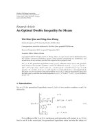
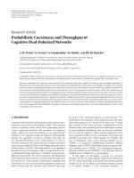
Figure 1: Proposed elliptical model.
3. Proposed Channel Model
The proposed channel model, shown in Figure 1,isbased
on the elliptical channel model first introduced in [2]. The
original model was intended for modelling a mobile to
basestation channel in a microcell, where the basestation is
not very high as in macrocells and a line of sight may exist.
Similar conditions are common in vehicular networks. The
number and position of the surroundings depend on the
terrain type. For highways, we expect a small number of
surroundings; the scatterers increase as we approach the city
where a large number of scatterers are more appropriate. The
surroundings are placed uniformly within two ellipses. The
parameters, a

m
and b
m
, of the outer ellipse are calculated
from the delay spread using the following equations [6],
while the inner ellipse is specified by the road geometries.
a
m
=
cτ
m
2
,
b
m
=
1
2

c
2
τ
2
m
−D
2
,
τ
m
= 3.244 σ

t
+ τ
0
,
(2)
where τ
m
is the maximum delay to be considered, σ
t
is
the delay spread, τ
0
is the minimum delay (line of sight
delay), D is the distance between the transmitter and receiver,
and c is the speed of light. The delay spread of VANET
hasbeenmeasuredforvariousroadsandtraffic conditions
in [9, 10]. The minimum mean delay spread measured
was 103 nanoseconds. We adopt this value in our model as
a worst-case scenario since a larger delay spread leads to
smaller antenna correlation.
We assume that the existence of objects (cars) between
the transmitter and receiver leads to blockage of line of sight.
When a line of sight exists, a ground reflection is added if the
distance between the transmitter and the receiver satisfies the
following equation:
D
≥
4π · h
t
·h

r
λ
,(3)
where h
t
and h
r
are the heights of the transmitter and receiver
antennas, respectively, and λ is the wavelength. The right-
hand side of (3) is the minimum distance for the first Fresnel
zone to touch the ground, and thus a ground reflection may
exist only if (3)issatisfied[11, 12].
EURASIP Journal on Wireless Communications and Networking 3
3210−1−2−3
Doppler frequency (normalized to Jakes’ maximum)
0
0.1
0.2
0.3
0.4
0.5
0.6
0.7
0.8
0.9
1
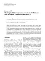
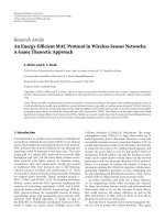
Doppler power spectral density
Figure 2: Channel autocorrelation function for proposed elliptical
and Jakes’ models.
The surroundings are not assumed fixed but their speeds

are uniformly distributed between 0 and a maximum limit.
For simplicity, we set the speed of the transmitter and sur-
roundings relative to the speed of the receiver. Surroundings
above the transmitter in Figure 1 are either fixed or moving
in a direction opposite to the transmitter (negative speed)
while those below the transmitter are either fixed or moving
in the same direction as the transmitter (positive speed). It
can be easily shown that the Doppler shift for any path (i)
is given by (4)or(5)[13, 14]. Equation (5)followsfrom
(4) since the last term in (4) is much smaller than the first.
Considering the elliptical model in Figure 1, the maximum
Doppler shift is no longer defined only by the relative speed
of the transmitter/receiver (v
T
-v
R
)asinJakes’modelbecause
the surroundings are not fixed [3, 14].
f
d
(i) = f

1+
v
T
−v
i
c
·cos


α
i


·

1+
v
i
−v
R
c
·cos

β
i


−
f ,
f
d
(i) =
f
c

v
T
−v
i


·
cos

α
i

+

v
i
−v
R

·
cos

β
i

+
f
c
2

v
T
−v
i


v
i
−v
R

cos

α
i

cos

β
i

,
(4)
f
d
(i) ≈
f
c

v
T
−v
i

·
cos


α
i

+

v
i
−v
R

·
cos

β
i

. (5)
The channel response (h(t)) at time (t)canberepresentedby
h(t)
=
N

i=0
g
i
·exp

j


2π · f
d
(i) · t
c
+ θ
i
+ ϕ
i

·
u

t −t
i

,
(6)
where g
i
is the reflection coefficient, t
i
and θ
i
are the excess
distance delay and phase, respectively, ϕ
i
is a random phase,
N is the number of paths, and u(t) is the unit step function.
The line of sight is represented by the i
= 0term.

109876543210
Spacing (
∗
λ)
0
0.1
0.2
0.3
0.4
0.5
0.6
0.7
0.8
0.9
1
Correlation coefficient
k = 0
k
= 4
k
= 6
k
= 8
k
= 10
Mathematical
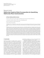
Figure 3: Antenna correlation versus spacing for sample line of
sight strengths, with ground reflection.
4. Model Statistics and Antenna Correlation
For our simulations, we use 10 scatterers. The maximum

speed was set to 120 km/h with the transmitter moving at
90 km/h and fixed receiver. The ratio of the line of sight
component to any of the other scatters is equal to k.The
delay spread is 103 nanoseconds as measured in [9]. The
distance (D) between the transmitter and receiver is 1 km,
which is the maximum transmission range specified for IEEE
802.11p [15], and the heights of the antennas were set to
1.5 m. The frequency is 5.9 GHz as specified by ASTM [16].
The amplitude distribution of the received signal using our
model was found to follow Rayleigh distribution for no
line of sight and Rician distribution when a line of sight
component exists. This agrees with the statistics obtained
from measurements in [11, 17]. The Rician distribution can
be approximated by a Gaussian distribution under strong
line of sight conditions [4].
The Doppler spectrum is shown in Figure 2. Comparing
Figure 2 with the classical Jakes spectrum [3], we observe
that the maximum Doppler shift exceeds that suggested
by Jakes due to the movement of the scatterers. In Jakes’
Doppler spectrum, the spectrum is bounded by f
d
given in
(1), whereas in VANET, the spectrum extends beyond this
value as observed from Figure 3.Thiseffect appears in the
autocorrelation function as faster variation compared to that
of Jakes’ model. Both models give identical results if the
speeds of the scatterers are set to zero. Similar conclusions
were reached in [18] via measurements.
The correlation between two antennas (ρ
ij

)canbe
calculated theoretically for Rayleigh fading using the AOA
probability distribution p(α) and the equation [19]
ρ
ij
=

2π
0
e
j((2·π)/λ)d cos(ϕ−ψ)
· p(ϕ) · dϕ,(7)
4 EURASIP Journal on Wireless Communications and Networking
where d is the spacing between the antennas and ψ is the
angle of orientation of the array (set to π/2 for broadside
and 0 for end fire). For mobile terminals, the surroundings
are usually assumed to be uniformly distributed in a circle
around the terminal (Lee’s model) leading to the AOA
distribution of the following equation [19]:
p(ϕ)
=
⎧
⎪
⎨
⎪
⎩
1
2π
,0
≤ ϕ ≤ 2π,

0, otherwise.
(8)
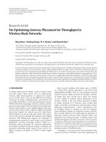
Figure 3 compares the correlation between the antennas
under various line of sight strengths and no line of sight
conditions using the elliptical model with the correlation
from (7). As can be seen, (7) gives an optimistic estimate
of the correlation due to the assumption of uniform angle
distribution which is realistic only in rich scattering channels.
We also note that the correlation increases as the line of
sight strength increases since the received signal becomes
dominated by the line of sight component. The ground
reflection reduces the correlation since the attenuation for
line of sight is inversely proportional to D
4
instead of D
2
,thus
the contribution of line of sight is reduced [11, 12]. Without
ground reflection, the correlation becomes higher, and it
is not possible to reduce it unless very large, impractical
antenna spacings are used.
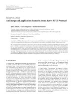
Although the line of sight condition is ideal for single
antenna systems, it can lead to severe degradation in the
performance of BLAST systems [19–21]. To illustrate this,
we used the channel model without ground reflection to
simulate a 2
× 4 VBLAST system using PSK modulation,
1 MHz bandwidth, and perfect channel knowledge. As shown
in Figure 4, the performance drops as the line of sight
increases. This is due to the correlation between the antennas

which leads to the loss of the diversity since the antennas
receive similar signals. In the next section, we introduce the
proposed channel update algorithm.
5. Channel Update
The performance of MIMO systems depends on the accuracy
of channel state information (CSI). In a fast varying channel,
the channel estimate must be updated more frequently.
Generally, a training sequence is used for channel estimation
[22–24]; however under fast varying conditions, the interval
between successive training sequences becomes small, and
thus the efficiency is reduced. Our aim in this section is to
develop an algorithm to update the channel estimate using
the received signal in order to increase the interval between
successive training intervals.
Several channel tracking algorithms are available for
single and multiple antenna systems. In [25], a maximum
likelihood channel tracking algorithm has been proposed.
Kalman filters have been considered in several papers. In
[26], the authors combined a Kalman filter with a decision
feedback equaliser (DFE). The DFE is used to estimate the
transmitted signal, and its output is fed to the Kalman
filter for channel tracking. In [27], an autoregressive moving
average (ARMA) filter was used to model the channel
20181614121086420
E
s
/N
0
(dB)
10

−5
10
−4
10
−3
10
−2
10
−1
10
0
BER
k = 0
k
= 2
k
= 3
k
= 4
k
= 6
k
= 8
Figure 4: Performance of VBLAST for various line of sight
strengths.
response based on Jakes’ channel power spectral density;
this was then used to design a Kalman filter for tracking.
The main limitation of these algorithms is complexity. The
decoding algorithms for MIMO systems are usually very
complicated and, therefore, it is desirable to minimise the

channel estimation and tracking complexity. In this section,
we develop a simple single tap Kalman filter to update the
channel and thus reduce the BER while keeping the increase
in hardware complexity to minimum.
For a p
× q VBLAST system with p transmit and q receive
antennas, q
≥ p, in a flat fading channel, the received signal
vector of length q (r
n−1
) at time index n −1canbewrittenas
r
n−1
= H
n−1
s
n−1
+ m
n−1
,(9)
where H
n−1
is the q × p channel matrix, s
n−1
is the column
vector of p transmitted symbols, and m
n−1
is the column
vector of q white noise samples at time n
−1. Unless otherwise

specified, bold upper-case characters represent matrices
and bold lower-case characters represent vectors while
normal lower-case characters represent elements within the
matrix/vector of the same character. Our analysis assumes
that the antenna separation is large enough for the received
signalstobeuncorrelated.
Let the estimated channel matrix be

H
n−1
. The simplest
BLAST receiver (zero-forcing receiver) calculates an estimate
of the transmitted symbols (
s
n−1
) using the pseudoinverse of
the channel matrix (

H
+
n
−1
)as[28]
s
n−1
=

H
+
n

−1
×r
n−1
. (10)
Define ΔH
n
as
ΔH
n
=

r
n−1
−

H
n−1
s
n−1

×s
+
n
−1
. (11)
EURASIP Journal on Wireless Communications and Networking 5
Substituting (9)in(11) and assuming correct decoding, we
find
ΔH
n

=

H
n−1
−

H
n−1

×
s
n−1
s
+
n
−1
+ m
n−1
s
+
n
−1
. (12)
Note that the term (r
n−1
−

H
n−1
s

n−1
) is calculated in the
cancellation step of the VBLAST decoding algorithm. ΔH
n
can be used with a first-order Kalman [13] filter to improve
the channel estimation as

H
n
=

H
n−1
+ K ·ΔH
n
, (13)
where K is a q
× p matrix of update parameters and the dot
in (13) represents the element-by-element multiplication.
We now need to find the optimum value of K,however,
since we assume that the receive antennas are not correlated;
we need to optimise for only one antenna. Equation (12)can
be rewritten for the elements of the matrix ΔH
n
as
Δh
n
ij
=


r
n−1
i
−
p

l=1

h
n−1
il
·s
n−1
l

a
n−1
j
. (14)
The subscripts identify the row (i)andcolumn(j or l)
which represent receive and transmit antennas, respectively,
while the superscript (n) denotes the time index. a
j
is the
element at column j of the row vector (
s
+
). Equation (14)
can be expanded using (9)as
Δh

n
ij
=

p

l=1

h
n−1
il
·s
n−1
l
−

h
n−1
il
·s
n−1
l
+ m
n−1
i


a
n−1
j

, (15)
and assuming correct decoding as
Δh
n
ij
=

p

l=1

h
n−1
il
−

h
n−1
il

·
s
n−1
l

a
n−1
j
+ m
n−1

i
a
n−1
j
= βε
n−1
ij
+
p

l=1
l
/
= j
ε
n−1
il
·s
n−1
l
·a
n−1
j
+ m
n−1
i
a
n−1
j
.

(16)
Here, ε
n−1
ij
= h
n−1
ij
−

h
n−1
ij
,andβ is the product of the s
n−1
j
and a
n−1
j
terms. The elements of the updated channel can be
written as

h
n
ij
=

h
n−1
ij
+ k

ij
Δh
n
ij
, (17)

h
n
ij
=

h
n−1
ij
+ βk
ij
ε
n−1
ij
+ k
ij
p

l=1
l
/
= j
ε
n−1
il

s
n−1
l
a
n−1
j
+ k
ij
m
n−1
i
a
n−1
j
.
(18)
With the assumption of independent identically dis-
tributed (i.i.d) white data and equal average signal to noise
ratio (SNR) for the receive antennas, the last two terms in
(18) can be approximated by white noise with average power
[13]:
N
0,j
=
P
0
ρ
j
⎛
⎜

⎜
⎜
⎝
1+
p

l=1
l
/
= j
e
l
⎞
⎟
⎟
⎟
⎠
, (19)
where P
0
is the original noise to signal power ratio for
receive antenna i, e
l
is the average error covariance reduction
value, and ρ
j
is a constant that specifies the fraction of noise
associated with stream j.Theoptimumvalueofk
ij
is the

one that minimises the expression E[
|h
n
ij
−

h
n
ij
|
2
]. For f
D
T
s
<
0.2, T
s
is the symbol duration, the channel autocorrelation
function (A(mT
s
)) can be approximated by (20)[29, 30].
Theoptimumvalueofk
ij
is then found using (21)to(24),
A

mT
s


≈
1 − π
2
f
2
D
T
2
s
·m
2
, (20)
k
ij
= k
j
∀i
,
(21)
k
j
= 3.6 ×
3





ρ
j


f
D
T
s

2
βP
0

1+

p
l
=1,l
/
= j
e
l

=
3.6 ×
3






f

D
T
s

2
P
0

1+

p
l
=1,l
/
= j
e
l

,
(22)
e
j
≈
0.75
p
k
j
,
(23)
P

0
=
1
E
s
/N
0
. (24)
We define E
s
/N
0
as the total SNR if all transmitting
antennas transmit the same symbol. We set β and ρ
j
equal to
1/p in (22)sinceweassumeequalaveragetransmit(receive)
power for each transmit (receive) antenna. The k
j
parameters
are calculated recursively. First, we assume no interference
from the other symbols and set e
j
= 0. This is best suited
for the last decoded symbol in VBLAST since all the other
symbols would be cancelled out by then. We then calculate k
j
and e
j
for this stream. Next, we substitute the new value of e

j
for the next to last decoded symbol and calculate the k
j
then
update e
j
. After all the initial k
j
parameters are calculated, the
processisrepeatedagainwithe
j
from the calculated k
j
. This
process converges very quickly, and the final values of k
j
are
not very different from the initial ones. The parameters then
can be used to update the channel estimate. The algorithm
requires the calculation of pk
j
parameters, one for each
transmit antenna (21)and(24). These can be calculated
once at the beginning of the packet and held constant for
the duration of the packet. ΔH
n
requires the pseudoinverse
of the (p
× 1) vector s, which can be precalculated and
stored, and then multiplying it by the term (r

n−1
−

H
n−1
s
n−1
),
(11), which is calculated in the VBLAST algorithm. This
multiplication consists of p
× q complex multiplication.
The update algorithm, (13), requires p
× q real-by-complex
multiplication and p
× q complex addition.
A simple analysis shows that the algorithm requires
6p
× q real multiplications and 4p × q real additions per
update. Assuming a 2
×4 system, the algorithm then requires
48 multiplications and 32 additions. If channel update is
conducted for every symbol, then a chosen 500 MHz DSP
processor, which executes a multiplication in 1 cycle, can
compute the update in 160 nanoseconds.
6 EURASIP Journal on Wireless Communications and Networking
26242220181614121086420
E
s
/N
0

(dB)
10
−5
10
−4
10
−3
10
−2
MSE
256
512
1024
256 no update
Figure 5: MSE of channel estimation for 180 km/h.
We ran a number of simulations using Matlab for a 2 ×
4 VBLAST system with a symbol rate of 1 MSymbol/s and
the elliptical channel model. The frequency was 5.9 GHz.
In our simulations, initially the algorithm would have
perfect channel knowledge rather than estimating from a
training sequence. This is necessary to isolate any errors that
might arise from the use of training sequence estimation.
The initial values of k
j
were used to reduce complexity,
and the channel estimate was updated for every sym-
bol.
Figure 5 shows the mean square error in the estimated
channel for the cases of 256, 512, and 1024 symbols per
antenna using QPSK modulation with channel update, using

(12)andfrom(21)to(24), compared to 256 without update.
As can be seen from Figure 5, the update algorithm reduces
the MSE by 50% at 12 dB E
s
/N
0
. The MSE in Figure 5
without update does not depend on the SNR because the
receiver is assumed to have perfect noise-free estimate of
the channel at the beginning of the packet, and this is held
constant for the duration of the packet. Figure 6 shows the
MSE versus the symbol number for 26 dB E
s
/N
0
. Initially,
the receiver will have perfect channel knowledge (MSE
≈
0) but with time this estimate becomes invalid due to the
high Doppler shift. If a training sequence was used, the
initial MSE will be greater than 0, thus shifting the curves
upwards. The difference between the curves, however, will
not change and, therefore, the MSE comparison will still
hold.
Figure 7 shows the BER performance of QPSK for various
relative vehicle speeds. As can be seen, the performance
improves considerably when the algorithm is used and is
2 dB from that of perfect channel knowledge for 60 km/h.
Figure 8 shows the performance of the same system using
QPSK with various packet lengths for a speed of 60 km/h.

120010008006004002000
Symbol number
10
−8
10
−7
10
−6
10
−5
10
−4
10
−3
10
−2
MSE
No update
With update
Thin line 100 kph
Thick line 180 kph
Figure 6: MSE of channel estimation versus the number of symbols
at 26 dB.
242220181614121086420
E
s
/N
0
(dB)
10

−5
10
−4
10
−3
10
−2
10
−1
10
0
BER
Perfect CSI
No update, 60 km/h
Update, 180 km/h
Update, 100 km/h
Update, 60 km/h
Figure 7: QPSK BER with and without channel update.
From Figure 8, we observe that the performance degrades
as the packet length increases; this is due to two reasons.
The first reason is estimation error, as the estimation process
proceeds, the error in the estimation accumulates, and for
long packets this will lead to erroneous results near the
end of the packet. The second reason is detection errors
since the probability of symbol errors increases as the packet
length increases. The estimation algorithm assumes correct
decoding; therefore, such errors will affect the performance
of the algorithm.
EURASIP Journal on Wireless Communications and Networking 7
2520151050

E
s
/N
0
(dB)
10
−5
10
−4
10
−3
10
−2
10
−1
10
0
BER
1024
512
256
Figure 8: BER for different packet sizes, 60 km/h.
6. Conclusion
In this paper, we introduced a channel model for vehicular
networks. The model was compared to Jakes’ model, and
it was shown that the Doppler power spectrum extends
beyond Jakes’ maximum frequency due to the movement of
the surroundings, transmitter, and receiver. The correlation
between antennas was then studied, and the results show that
under very strong line of sight conditions, the correlation is

high and, therefore, a small gain is expected from the use of
multiple antennas while for moderate and no line of sight
conditions the correlation is low. We also developed a simple
recursive algorithm to keep track of changes in the channel
and update the channel estimation matrix for VBLAST. The
update algorithm enhances the channel estimation on a
symbol-by-symbol basis, but this can be relaxed for high
symbol rates and/or slow fading as the channel coherence
time will be large compared to the symbol duration. The
proposed algorithm improves system BER and channel
estimate MSE via continuous and accurate channel updating
and has less computational complexity compared to existing
tracking algorithms as a result of using a simplified Kalman
filter. Simulation results showed remarkable improvements
when using the update algorithm compared to the training
of only channel estimation. The algorithm is capable of
updating the channel estimation for VBLAST for nodes
moving at high speeds thus improving the bit error rate and
reliability of VANET.
Acknowledgment
The authors would like to thank France Telecom and the
University of Plymouth for supporting this work as well as
the anonymous reviewers for their valuable comments.
References
[1] S. Haykin and M. Moher, Modern Wireless Communications,
Prentice-Hall, Upper Saddle River, NJ, USA, 2005.
[2] J.C.LibertiandT.S.Rappaport,“Ageometricallybasedmodel
for line-of-sight multipath radio channels,” in Proceedings of
the 46th IEEE Vehicular Technology Conference (VTC ’96), vol.
2, pp. 844–848, Atlanta, Ga, USA, April-May 1996.

[3] W. C. Jakes, Microwave Mobile Communications, IEEE Press,
Piscataway, NJ, USA, 1994.
[4] J. D. Parsons, TheMobileRadioPropagationChannel,John
Wiley & Sons, New York, NY, USA, 2001.
[5]W.C.Y.Lee,Mobile Communications Engineering, McGraw-
Hill, New York, NY, USA, 1982.
[6]R.B.Ertel,P.Cardieri,K.W.Sowerby,T.S.Rappaport,and
J. H. Reed, “Overview of spatial channel models for antenna
array communication systems,” IEEE Personal Communica-
tions, vol. 5, no. 1, pp. 10–22, 1998.
[7]C.S.Patel,G.L.St
¨
uber, and T. G. Pratt, “Simulation of
Rayleigh-faded mobile-to-mobile communication channels,”
IEEE Transactions on Communications, vol. 53, no. 11, pp.
1876–1884, 2005.
[8]A.G.Zaji
´
c and G. L. St
¨
uber, “A three-dimensional MIMO
mobile-to-mobile channel model,” in Proceedings of the
IEEE Wireless Communications and Networking Conference
(WCNC ’07), pp. 1885–1889, Hong Kong, March 2007.
[9]D.W.Matolak,I.Sen,W.Xiong,andN.T.Yaskoff,“5GHZ
wireless channel characterization for vehicle to vehicle com-
munications,” in Proceedings of IEEE Military Communications
Conference (MILCOM ’05), vol. 5, pp. 3022–3016, Atlatnic
City, NJ, USA, October 2005.
[10] A. Paier, J. Karedal, N. Czink, et al., “Car-to-car radio chan-

nel measurements at 5 GHz: pathloss, power-delay profile,
and delay-Doppler spectrum,” in Proceedings of 4th IEEE
Internatilonal Symposium on Wireless Communication Systems
(ISWCS ’07), pp. 224–228, Trondheim, Norway, October 2007.
[11] L. Cheng, B. E. Henty, D. D. Stancil, F. Bai, and P. Mudalige,
“Mobile vehicle-to-vehicle narrow-band channel measure-
ment and characterization of the 5.9 GHz dedicated short
range communication (DSRC) frequency band,” IEEE Journal
on Selected Areas in Communications, vol. 25, no. 8, pp. 1501–
1516, 2007.
[12] A. Polydoros, K. Dessouky, J. M. N. Pereira, et al., “Vehicle
to roadside communications study,” Research Reports UCB-
ITS-PRR-93-4, California Partners for Advanced Transit and
Highways (PATH), University of California, Berkeley, Calif,
USA, June 1993.
[13] F. T. Ulaby, Fundamentals of Applied Electromagnetics,
Prentice-Hall, Upper Saddle River, NJ, USA, 1999.
[14] T. P. Gill, The Doppler Effect, Logos Press, New York, NY, USA,
1965.
[15] IEEE Draft P802.11p/D2.0, November 2006.
[16] American Society for Testing and Materials (ASTM),
/>[17]J.Maurer,T.F
¨
ugen, and W. Wiesbeck, “Narrow-band
measurement and analysis of the inter-vehicle transmission
channel at 5.2 GHz,” in Proceedings of the 55th IEEE Vehicular
Technology Conference (VTC ’02), vol. 3, pp. 1274–1278,
Birmingham, Ala, USA, May 2002.
[18] L. Cheng, B. E. Henty, D. D. Stancil, and F. Bai, “Doppler
component analysis of the suburban vehicle-to-vehicle DSRC

propagation channel at 5.9 GHz,” in Proceedings of the IEEE
Radio and Wireless Symposium (RWS ’08), pp. 343–346,
Orlando, Fla, USA, January 2008.
8 EURASIP Journal on Wireless Communications and Networking
[19] D. Chizhik, F. Rashid-Farrokhi, J. Ling, and A. Lozano, “Effect
of antenna separation on the capacity of BLAST in correlated
channels,” IEEE Communications Letters, vol. 4, no. 11, pp.
337–339, 2000.
[20] D. Chizhik, G. J. Foschini, M. J. Gans, and R. A. Valen-
zuela, “Keyholes, correlations, and capacities of multielement
transmit and receive antennas,” IEEE Transactions on Wireless
Communications, vol. 1, no. 2, pp. 361–368, 2002.
[21] X. Li and Z. Nie, “Performance losses in V-BLAST due to
correlation,” IEEE Antennas and Wireless Propagation Letters,
vol. 3, no. 1, pp. 291–294, 2004.
[22] M. Biguesh and A. B. Gershman, “Training-based MIMO
channel estimation: a study of estimator tradeoffs and optimal
training signals,” IEEE Transactions on Signal Processing, vol.
54, no. 3, pp. 884–893, 2006.
[23] H. Minn and N. Al-Dhahir, “Optimal training signals for
MIMO OFDM channel estimation,” IEEE Transactions on
Wireless Communications, vol. 5, no. 5, pp. 1158–1168, 2006.
[24] B. Park and T. F. Wong, “Optimal training sequence in MIMO
systems with multiple interference sources,” in Proceedings
of the IEEE Global Telecommunications Conference (GLOBE-
COM ’04), vol. 1, pp. 86–90, Dallas, Tex, USA, November-
December 2004.
[25] E. Karami and M. Shiva, “Maximum likelihood MIMO
channel tracking,” in Proceedings of the 59th IEEE Vehicular
Technology Conference (VTC ’04), vol. 2, pp. 876–879, Milan,

Italy, May 2004.
[26] G. Yanfei and H. Zishu, “MIMO channel tracking based
on Kalman filter and MMSE-DFE,” in Proceedings of the
International Conference on Communications, Circuits and
Systems (ICCCAS ’05), vol. 1, pp. 223–226, Hong Kong, May
2005.
[27] L. Li, H. Li, H. Yu, B. Yang, and H. Hu, “A new algorithm
for MIMO channel tracking based on Kalman filter,” in Pro-
ceedings of the IEEE Wireless Communications and Networking
Conference (WCNC ’07), pp. 164–168, Hong Kong, March
2007.
[28] D. Gore, R. W. Heath Jr., and A. Paulraj, “On performance of
the zero forcing receiver in presence of transmit correlation,”
in Proceedings of IEEE International Symposium on Information
Theory (ISIT ’02), p. 159, Lausanne, Switzerland, June-July
2002.
[29]H.Meyr,M.Moeneclaey,andS.A.Fechtel,Digital Commu-
nication Receivers, John Wiley & Sons, New York, NY, USA,
1998.
[30]T.Wang,J.G.Proakis,E.Masry,andJ.R.Zeidler,“Per-
formance degradation of OFDM systems due to doppler
spreading,” IEEE Transactions on Wireless Communications,
vol. 5, no. 6, pp. 1422–1432, 2006.