Báo cáo hóa học: " Research Article An Iterative Soft Bit Error Rate Estimation of Any Digital Communication Systems Using a Nonparametric Probability Density Function" pptx
Bạn đang xem bản rút gọn của tài liệu. Xem và tải ngay bản đầy đủ của tài liệu tại đây (658.41 KB, 9 trang )
Hindawi Publishing Corporation
EURASIP Journal on Wireless Communications and Networking
Volume 2009, Article ID 512192, 9 pages
doi:10.1155/2009/512192
Research Article
An Iterative Soft Bit Error Rate Estimation of Any Digital
Communication Systems Using a Nonparametric Probability
Density Function
Samir Saoudi,
1, 2
Molka Troudi,
3
and Faouzi Ghorbel
4
1
Institut TELECOM, TELECOM Bretagne, UMR CNRS 3192 Lab-STICC, Technop
ˆ
ole Brest-Iroise CS 83818,
29238 Brest Cedex
∼3, France
2
Universit
´
eEurop
´
eenne de Bretagne, (UeB), France
3
Institut TELECOM, TELECOM Bretagne, Technop
ˆ
ole Brest-Iroise CS 83818, 29238 Brest Cedex∼3, France
4
Laboratoire CRISTAL, Ecole Nationale de Sciences de L’Informatique (ENSI), Campus Universitaire de la Manouba,
2010 Manouba, Tunisia
Correspondence should be addressed to Samir Saoudi,
Received 22 July 2008; Accepted 3 March 2009
Recommended by Sangarapillai Lambotharan
In general, performance of communication system receivers cannot be calculated analytically. The bit error rate (BER) is thus
computed using the Monte Carlo (MC) simulation (Bit Error Counting). It is shown that if we wish to have reliable results with
good precision, the total number of transmitted data must be conversely proportional to the product of the true BER by the
relative error of estimate. Consequently, for small BERs, simulation results take excessively long computing time depending on the
complexity of the receiver. In this paper, we suggest a new means of estimating the BER. This method is based on an estimation, in
an iterative and nonparametric way, of the probability density function (pdf) of the soft decision of the received bit. We will show
that the hard decision is not needed to compute the BER and the total number of transmitted data needed is very small compared
to the classical MC simulation. Consequently, computing time is reduced drastically. Some theoretical results are also given to
prove the convergence of this new method in the sense of mean square error (MSE) criterion. Simulation results of the suggested
BER are given using a simple synchronous CDMA system.
Copyright © 2009 Samir Saoudi et al. This is an open access article distributed under the Creative Commons Attribution License,
which permits unrestricted use, distribution, and reproduction in any medium, provided the original work is properly cited.
1. Introduction
The famous Monte Carlo (MC) simulation technique is the
most popular technique used for estimating bit error rate
(BER) of digital communication systems. The MC method is
used when we cannot analytically compute the performance
of communication system receivers. Unfortunately, it is well
known that the drawback of the MC method is its very
high computational cost. If we are studying, for example,
a channel with a BER equal to 10
−6
, it is shown that if
we hope to have a relative error estimation equal to 10
−1
,
the number of the incorrect received bits must be at least
equal to 10
2
and then the total number of transmitted
data must be at least equal to 10
8
(see [1]). Consequently,
simulation results take excessively long computing time. In
this paper, we suggest a new method to estimate the BER
based on an estimation, in an iterative and nonparametric
way, of the probability density function (pdf) of the soft
decision of the received bit. In this case, the hard decision
is not needed to compute the BER. The total number of
transmitted data needed is very small compared to the
classical MC simulation. Consequently, computing time is
reduced drastically. The paper is organized as follows. In
Section 2, a brief review of the MC simulation method is
given. Section 3 shows how a pdf can be estimated in a
parametric way. Section 4 gives some details about the new
suggested iterative soft BER estimation. The convergence of
this new method in the sense of Mean Square Error (MSE)
criterion is discussed in Section 5. Simulation results are
presented in Section 6. Finally, a brief summary of the results
is given in Section 7.
2 EURASIP Journal on Wireless Communications and Networking
2. Monte Carlo Simulation: a Brief Review
In this section, we will give a brief description of the MC
simulation for any digital communication system. Let us
consider any point to point system communication over
any channel transmission (Gaussian, multipath fading, etc.)
with or without channel coding using any transmission tech-
niques (CDMA, MC-CDMA, TDMA, etc.). Let (b
i
)
1≤i≤N
∈
{
+1, −1} asetofN independent transmitted bits. Let
(X
i
)
1≤i≤N
be the corresponding soft output at the receiver
such as the decision is taken by using its sign:
b
i
= sgn(X
i
).
Let us introduce the following error function defined by
a Bernoulli random variable:
ξ
b
i
=
⎧
⎪
⎨
⎪
⎩
1if
b
i
/
=b
i
,
0 otherwise.
(1)
Let p
e
be the true BER at the output of the receiver. We
have
p
e
= Pr
b
i
/
=b
i
=
Pr
ξ
b
i
=
1
= E
ξ
b
i
,(2)
where
E(·) is the mathematical expectation operator. The
MC method estimates BER using the following average:
p
e
=
1
N
N
i=1
ξ
b
i
. (3)
Theestimatorerrorisgivenby
e
= p
e
−
p
e
=
1
N
N
i=1
(p
e
− ξ(b
i
)). (4)
The MC estimator is unbiased since
E(e) = 0and
its variance is given by (assuming that the errors are
independent)
σ
2
e
= E
p
e
−
p
e
2
=
p
e
1 − p
e
N
. (5)
Let ε be the relating error of the MC estimator which is
given by
ε
=
σ
e
E
p
e
=
1 − p
e
p
e
N
. (6)
For small BER (p
e
1), we have
ε
≈
1
p
e
N
. (7)
Equation (7) gives the number of transmitted data
needed for a given BER and for a desired precision ε:
N
=
1
ε
2
p
e
. (8)
It is clear from (8) that, for example, if we wish to
study a channel with a BER equal to 10
−7
with a desired
precision of 10
−1
,wemusttransmitatleast10
9
information
bits. Consequently, simulation results take excessively long
computing time depending on the complexity of the receiver.
So, small BER values require large samples length N. That is
why, in the following sections, we will suggest a new method
to estimate the BER based on nonparametric pdf of soft
output decision X.
3. Nonparametric Probability Density
Function Estimation
Let f
X
(x) be the pdf of the soft output decision X at the
receiver. Let us note that all the received soft output decision
(X
i
)
1≤i≤N
are random variables having the same pdf, f
X
(x).
X
i
is the corresponding soft output at the receiver such as
the hard decision is taken by using its sign:
b
i
= sgn(X
i
).
The (b
i
)
1≤i≤N
are assumed to be independent and identically
distributed with P[b
i
=±1] = 1/2. The BER is then given by
p
e
= P
b
i
/
=b
i
,
= P
(X>0),
b
i
=−1
+ P
(X<0),
b
i
= +1
,
= P
X>0 | b
i
=−1
P
b
i
=−1
+ P
X<0 | b
i
= +1
P
b
i
= +1
,
= P
X>0 | b
i
=−1
,
= P
X<0 | b
i
= +1
,
(9)
then,
p
e
=
0
−∞
f
b
i
=+1
X
(x)dx
=
+∞
0
f
b
i
=−1
X
(x)dx
=
1
2
0
−∞
f
b
i
=+1
X
(x)dx +
1
2
+∞
0
f
b
i
=−1
X
(x)dx,
(10)
where f
b
i
=+1
X
(·)(resp.,f
b
i
=−1
X
(·)) is the conditional pdf of X
such as b
i
= +1 (resp., b
i
=−1).
Equation (10) clearly shows that an alternative method
for estimating the BER is to transmit, for example, a sequence
of N bits equal to +1, estimate the pdf of the soft output of
the receiver and then calculate the BER by computing the
appropriate integral given by (10).
However, in a practical situation, the nature of the
pdf of the observed random variable X depends on both
the type of receiver and the channel model; Gaussian
function for a simple additive white Gaussian noise (AWGN)
channel, a mixture of Gaussian functions for an AWGN
CDMA receiver, or other distributions used for Rayleigh,
Nakagami, or Rice fading channels. In the case of advanced
receivers using iterative techniques or nonlinear filters such
as turbo codes for multiple input multiple output (MIMO)
systems [2], it is very difficult to find the right parametric
model for the received distribution. That is why, for any
communication systems, we suggest using nonparametric
methods to estimate the pdf of the observed data, X.In
fact, the most popular nonparametric pdf estimations are the
Kernel method [3, 4] or the orthogonal series estimators such
as the Fourier series [5]. Recent suggestions for methods can
be found in [6, 7] with applications for shape classification
and speech coding. In this paper, we will focus on the use of
the Kernel method and its use for estimating the BER.
EURASIP Journal on Wireless Communications and Networking 3
The Kernel estimator is defined as
f
X,N
(x) =
1
Nh
N
N
i=1
K
x −X
i
h
N
, (11)
where (X
i
)
1≤i≤N
are random variables having the same pdf,
f
X
(x). X
i
is the soft output at the receiver right before the
hard decision. h
N
is the smoothing parameter which depends
on the length of the observed samples, N. K(
·) is any pdf
(called the kernel) assumed to be an even and regular (i.e.,
square integrated) function with unit variance and zero
mean.
The choice of the smoothing parameter h
N
is very
important. It is shown in [6, 7] that if h
N
tends towards
0 when N tends towards +
∞, the estimator
f
X,N
(x)is
asymptotically unbiased (i.e., for all x,
E[
f
X,N
(x)] → f
X
(x)).
It is also shown that if h
N
→ 0andNh
N
→ +∞ when
N
→ +∞, then the MSE of the Kernel estimator tends to
zero, that is, for all x:
lim
N →+∞
E
f
X,N
(x) − f
X
(x)
2
=
0. (12)
Moreover, the optimal smoothing parameter h
N
is com-
puted in the minimum of the Integrated Mean Squared Error
(IMSE) sense. An approximation of the IMSE is given by the
following formula: (see [8])
IMSE
≈
M(K)
Nh
N
+
J
f
X
h
4
N
4
, (13)
where M(K)
=
+∞
−∞
K
2
(x)dx, J( f
X
) =
+∞
−∞
( f
X
(x))
2
dx and
f
X
(x) is the second derivative of the pdf f
X
(x). The optimal
smoothing value, h
∗
N
, is then given by minimising the IMSE.
We then obtain
h
∗
N
= N
−1/5
J
f
X
−1/5
(M(K))
+1/5
. (14)
Equation (14) shows that we must compute J( f
X
)which
unfortunately depends on the unknown pdf, f
X
. In the rest of
this paper, we suggest the use of the most popular Gaussian
kernel: K(x)
= (1/
√
2π)exp(−x
2
/2). In this case, using (11),
we have (proof is given in Appendix A)
J
f
X,N
=
1
N
2
h
5
N
√
2
N
i=1
N
j=1
K
X
i
− X
j
√
2h
N
X
i
− X
j
2h
N
4
+
3
4
.
(15)
Let us note that we can easily show that for a zero mean
and unit variance Gaussian kernel, we have
M(K)
=
+∞
−∞
K
2
(x)dx =
1
2
√
π
. (16)
4. Soft BER Estimation
To find the optimal smoothing parameter h
∗
N
,wemust
resolve (14) using at the same time (15)and(16). Direct
resolution seems to be very difficult. That is why we suggest
resolving this equation in an iterative way; we begin by an
initial value of h
N
(h
(0)
N
= 1/N
1/5
), then, for each iteration
k:computeJ(
f
X,N
) using (15) with the previous h
(k−1)
N
and
then compute the new value of h
(k)
N
by using (14). Once the
optimal smoothing parameter is calculated, the pdf
f
X,N
(x),
if needed, can be estimated by using (11). To estimate the
BER of our system, we must evaluate the expression of
(10):
p
e
=
0
−∞
f
X,N
(x)dx. We can show that for the chosen
Gaussian kernel, a soft BER estimation can be given by the
following expression (see proof in Appendix B):
p
e,N
=
1
N
N
i=1
Q
X
i
h
N
, (17)
where Q(
·) denotes the complementary unit
cumulative Gaussian distribution, that is, Q(x)
=
+∞
x
(1/
√
2π)exp(−t
2
/2)dt. The erfc function can also
be used as follows: Q(x)
= 1/2erfc(x/
√
2).
Let us now summarize the new suggested algorithm
which estimates the soft BER of any communication system:
Soft BER algorithm:Let(X
i
)
1≤i≤N
be the received soft out-
put decision (corresponding to an N transmitted sequence
bits equal to +1, so as the estimated pdf will be the
conditional one of X such as b
= +1).
(1) Initialization. h
(0)
N
= 1/N
1/5
.
(2) For each iteration k:(k
= 1, 2, )
(i) Compute J(
f
(k)
X,N
) using h
(k−1)
N
(15).
(ii) Compute h
(k)
N
using J(
f
(k)
X,N
)andM(K)((14)
and (16)).
(iii) STOP iteration criterion:
|h
(k)
N
− h
(k−1)
N
| <
threshold
≈ 10
−3
.
(3) Soft BER computation:(see(17)).
5. Some Theoretical Studies
In this section we shall give some theoretical studies. The
following theorem will show that the suggested soft BER
estimator is asymptotically unbiased. Proof of this theorem
is given in Appendix C.
Theorem 5.1. Assume that f
X
is a second derivative pdf
function, that h
N
→ 0 as N → +∞. Then
p
e,N
is
asymptotically unbiased, that is,
lim
N →+∞
E
p
e,N
=
p
e
. (18)
The following theorem shows that the variance of the
suggested estimator also tends to zero. Proof of this theorem
is given in Appendix D.
Theorem 5.2. Assume that f
X
is a second derivative pdf
function, that h
N
→ 0 as N → +∞. Then, the variance of
p
e,N
tends to zero as N tends to +∞,thatis,
lim
N →+∞
E
p
e,N
− E
p
e,N
2
=
0. (19)
4 EURASIP Journal on Wireless Communications and Networking
Using Theorems 5.1 and 5.2, it is easy to show (see
Appendix E) that the suggested estimator is pointwise consis-
tent, that is, the MSE tends to zero as the number of samples
N tends to +
∞. This result can be given by the following
corollary.
Corollary 5.3. Assume that f
X
is a second derivative pdf
function, that h
N
→ 0 as N → +∞.Then,theMSEof
p
e,N
tends to zero as N tends to +∞,thatis,
lim
N →+∞
E
p
e,N
− p
e
2
=
0. (20)
In the following, some remarks are given.
(1) Asymptotic normality: Using the central limit theo-
rem, we can show that the sequence of BER estimator
p
e,N
= (1/N)
N
i
=1
Q(X
i
/h
N
) is asymptotically normal,
that is,
∀c ∈ R,lim
N →+∞
P
p
e,N
− E
p
e,N
σ
p
e,N
≤
c
=
c
−∞
1
√
2π
exp
−
y
2
2
dy.
(21)
(2) Boostrap:As
f
X,N
(x) is constructed by the Kernel
estimator (11) for a given observation X
1
, X
2
, , X
N
,
with kernel K and bandwidth h
N
, then it is easy to
find new independent realizations from this estima-
tor. It is not necessary to explicitly compute
f
X,N
(x)
in the simulation procedure. New realizations Y can
be drawn as follows:
(i) uniformly choose an index i with replacement
from the set
{1, , N};
(ii) generate a random variable ε having K as a pdf;
(iii) Set Y
= X
i
+ εh
∗
N
.
These new realizations can be used to improve the accuracy
of the estimator and therefore reduce the variance of the
estimator.
6. Simulation Results
Let us consider a simple example in order to verify that
our suggested BER estimator works well. In this section,
we shall consider a synchronous CDMA system with K
users employing normalized spreading codes s
1
, s
2
, , s
k
∈
{−
1/
√
SF, +1/
√
SF}
SF
of length SF chips, through an AWGN
channel using binary phase-shift keying (BPSK), where SF is
the spreading factor. The received signal is the superposition
of the data signals of K users given by
r
=
K
k=1
A
k
b
k
s
k
+ n, (22)
where,
r
∈ R
SF
is the received signal (SF = spreading factor);
s
k
∈{+1/
√
SF, −1/
√
SF}
SF
is the spreading code for the
kth user;
b
k
∈{+1, −1} is the transmitted binary information
symbol of the kth user;
A
k
is the received amplitude of the kth user;
n
∈ R
SF
is an additive white Gaussian noise with
zero mean and a covariance matrix equal to σ
2
I
SF
,(n ∼
N (0,σ
2
I
SF
)).
It is seen [9] that a sufficient statistic for demodulating
the data bits of the K users is given by the K-vector y whose
kth component is the output of a filter matched to s
k
, that is,
y
k
= s
k
r, k = 1, , K. (23)
Using (22)and(23), we can show that the output of the
kth matched filter is given by
y
k
= A
k
b
k
+
j
/
=k
A
j
b
j
ρ
j,k
+ n
k
, (24)
where ρ
j,k
is the normalized cross-correlation between the
spreading codes s
j
and s
k
, n
k
is the output additive Gaussian
noise (
n
k
∼ N (0,σ
2
)).
Note that the quantity (24) consists of three terms:
the required bit information of the kth user, A
k
b
k
;a
term
j
/
=k
A
j
b
j
ρ
j,k
which is the multiple access interference
(MAI) at the output of the matched filter due to the presence
of other users sharing the same channel; and a term
n
k
,due
to the output of the background noise through the matched
filter. Let us note that the additive noise, MAI +
n
k
, at the
output of the kth matched filter is a mixture of 2
K−1
Gaussian
distribution.
Several multiuser detection methods are given in [9].
Here, we shall focus on the conventional detector which is
given by
b
k
= sign
y
k
. (25)
We can show, using (24), that the true bit error rate of
the kth user for the conventional detector is given by the
following formula:
BER
k
=
1
2
K−1
b
−k
∈{±1}
K−1
Q
A
k
−
j
/
=k
A
j
b
j
ρ
j,k
σ
,
(26)
where b
−k
= (b
1
, b
2
, , b
k−1
, b
k+1
, , b
K
) ∈{−1,+1}
K−1
.
For numerical results, we focus, for example, on K
=
2 users with SF = 7. The two spreading codes are
chosen as s
1
= (+1,+1, +1, +1, −1, −1, −1)/
√
7ands
2
=
(−1, −1, +1, +1, −1, −1, −1)/
√
7. We have found that the
cross-correlation value of these two codes is equal to ρ
1,2
=
0.4286. Figure 1 (resp., 2) gives the conditional pdf such as
b
1
= +1 of the output of matched filter for user k = 1andfor
aSNR
= 6 dB (resp., SNR = 10 dB).
Figure 3 gives performance of the conventional CDMA
detector based on the true bit error rate (see (26)) compared
with the method suggested in this paper and based on soft
EURASIP Journal on Wireless Communications and Networking 5
3210−1−2−3
Output of MF of user 1
0
0.1
0.2
0.3
0.4
0.5
0.6
0.7
Probability density function
Figure 1: Conditional pdf such as b
1
= +1 of the output of matched
filter for user k
= 1 and for an SNR = 6dB.
3210−1−2−3
Output of MF of user 1
0
0.1
0.2
0.3
0.4
0.5
0.6
0.7
0.8
0.9
Probability density function
Figure 2: Conditional pdf such as b
1
= +1 of the output of matched
filter for user k
= 1 and for a SNR = 10 dB.
BER algorithm given in Section 4. For this last simulation,
we have taken a database of length of N
= 1.000 samples.
The figure shows that for SNR
= 10 dB, 1000 samples are
sufficient to have a good precision of the bit error rate. For
SNR
= 10 dB, the true BER is equal to 3.010
−3
, therefore,
the MC simulation needs at least 30 000 samples for similar
precision.
Other Receiver. In this section, instead of using a simple
standard receiver, we shall consider a second example using
an MMSE receiver which is an advanced technique using
multiuser detection (see [9]). In this case, the output of the
MMSE receiver is given by
z
= My, (27)
1086420
SNR
= E
b1
/N
0
(dB)
Single user BER
Tr ue B ER of M F d etec to r
New soft BER estimator
10
−6
10
−5
10
−4
10
−3
10
−2
10
−1
10
0
BER
Figure 3: Soft BER algorithm and true BER comparison for
synchronous CDMA system.
where y = [y
1
, , y
K
]
is the K-dimensional vector of
matched filter outputs (y
k
is given by (24)). The MMSE filter
is given by
M
=
R + σ
2
A
−2
−1
, (28)
where R is the normalized cross-correlation matrix (R
i,j
=
s
i
s
j
= ρ
i,j
), A = diag{A
1
, , A
K
} and σ
2
is the variance of
the additive white Gaussian noise.
The estimated bit for the kth user (1
≤ k ≤ K) is then
given by
b
k
= sign
z
k
=
sign
My
k
. (29)
We can show, using (27) and the fact that y
= S
r (where
S
= [s
1
, , s
K
] is the N×K matrix of signature vectors), that
the true bit error rate of the kth user for the MMSE receiver
is given by the following formula:
BER
k
=
1
2
K−1
b
−k
∈{±1}
K−1
Q
(MR)
k,k
A
k
−
j
/
=k
(MR)
k, j
A
j
b
j
σ
(MRM)
k,k
,
(30)
where b
−k
= (b
1
, b
2
, , b
k−1
, b
k+1
, , b
K
) ∈{−1,+1}
K−1
.
For numerical results, we focus on K
= 2 users with
the same spreading codes chosen for the first simulation
(conventional detector). Let us note that the conditional pdf
such as b
1
= +1 of the output of MMSE filter for each user is
amixtureof2
K−1
Gaussian distribution.
Figure 4 gives performance of the MMSE receiver based
on the true bit error rate (see (30)) compared with the
method suggested in this paper and based on soft BER
algorithm given in Section 4. For this last simulation, we have
6 EURASIP Journal on Wireless Communications and Networking
876543210
SNR
= E
b1
/N
0
(dB)
Single user BER
MF detector
True BER of MMSE receiver
New soft BER estimator
10
−4
10
−3
10
−2
10
−1
10
0
BER of user 1
Figure 4: Soft BER algorithm and true BER comparison for
synchronous MMSE-CDMA receiver.
taken a database of length of N = 3.000 samples. The figure
shows that for SNR
= 6 dB, 3000 samples are sufficient to
have a good precision of the bit error rate. For such SNR, the
true BER is equal to 5.010
−3
, therefore, the MC simulation
needs at least 50 000 samples for similar precision. Let us also
note that for SNR
= 8dB,Figure 4 shows that the true BER
is equal to 6.010
−4
. In this case, the MC simulation needs
at least 170 000 samples for a good precision. The soft BER
estimation, by using only 3000 samples, gives a value of the
BER with an error of 0.2dB.
7. Conclusions
In this paper, we have suggested a new iterative soft bit error
rate estimation for the study of any digital communication
system performance. This method is based on the use of
nonparametric pdf estimation of the soft decision of the
received bit. Small length of transmitted data, compared
to the MC method, is needed for the BER estimation.
Convergence of this method in the MSE criterion has
been proven. Some simulation results have been given in
synchronous CDMA system case with both conventional
detector and MMSE multiuser receiver.
Appendices
A. Proof of (15)
Proof. Using the definition of J( f
X
), we have
J
f
X,N
=
+∞
−∞
f
X,N
(x)
2
dx. (A.1)
For Gaussian Kernel K, we have, K
(x) = (x
2
−1)K(x). Then,
using (11), we have
J
f
X,N
=
1
N
2
h
6
N
N
i=1
N
j=1
+∞
−∞
x −X
i
h
N
2
− 1
×
x −X
j
h
N
2
− 1
×
K
x −X
i
h
N
K
x −X
j
h
N
dx,
=
1
N
2
h
6
N
N
i=1
N
j=1
+∞
−∞
x −X
i
h
N
2
− 1
×
x −X
j
h
N
2
− 1
×
K
2x −
X
i
+ X
j
√
2h
N
K
X
i
− X
j
√
2h
N
dx.
(A.2)
Let us use the following change of variable: t
= [2x−(X
i
+
X
j
)]/
√
2h
N
and let us note a
i,j
= (X
i
− X
j
)/2h
N
.wehave
x −X
j
h
N
2
− 1
x −X
j
h
N
2
− 1
=
t
4
4
+ t
2
2a
2
i,j
− 1
+
a
2
i,j
− 1
2
.
(A.3)
Using both (A.2)and(A.3), we obtain
J
f
X,N
=
1
N
2
h
5
N
√
2
N
i=1
N
j=1
K
√
2a
i,j
×
+∞
−∞
t
4
4
+ t
2
2a
2
i,j
− 1
+
a
2
i,j
− 1
2
K(t)dt.
(A.4)
For a zero mean and unit variance Gaussian Kernel, the
second and fourth moment are, respectively, equal to 1 and
3, that is,
t
2
K(t)dt = 1and
t
4
K(t)dt = 3. Therefore, (A.4)
becomes
J(
f
X,N
) =
1
N
2
h
5
N
√
2
N
i=1
N
j=1
K
√
2a
i,j
a
4
i,j
+
3
4
. (A.5)
B. Proof of (17)
Proof. We must evaluate the expression of (10) in the case
where
f
X,N
is estimated by Kernel method (see (11)). Then,
p
e,N
=
0
−∞
f
X,N
(x)dx,
=
0
−∞
1
Nh
N
N
i=1
K
x −X
i
h
N
dx.
(B.1)
EURASIP Journal on Wireless Communications and Networking 7
By using the following change of variable, t
= (x − X
i
)/h
N
,
we have
p
e,N
=
0
−∞
1
Nh
N
N
i=1
K
x −X
i
h
N
dx
=
N
i=1
(−X
i
/h
N
)
−∞
1
N
K(t)dt
=
1
N
N
i=1
(−X
i
/h
N
)
−∞
1
√
2π
e
−(t
2
/2)
dt
=
1
N
N
i=1
+∞
(X
i
/h
N
)
1
√
2π
e
−(t
2
/2)
dt
=
1
N
N
i=1
Q
X
i
h
N
.
(B.2)
C. Proof of Theorem 5.1
Proof. Let us first recall that the true BER is given by
p
e
=
0
−∞
f
X
(x)dx. (C.1)
The suggested soft BER estimator is given by
p
e,N
=
0
−∞
1
Nh
N
N
i=1
K
x −X
i
h
N
. (C.2)
Then,
E
p
e,N
=
0
−∞
1
Nh
N
N
i=1
E
K
x −X
i
h
N
dx
=
0
−∞
1
Nh
N
NE
K
x −X
1
h
N
dx
=
0
−∞
1
h
N
+∞
−∞
K
x −u
h
N
f
X
(u)du
dx.
(C.3)
Using the following change of variable t
= (x −u)/h
N
,we
have
E
p
e,N
=
0
−∞
1
h
N
+∞
−∞
K(t) f
X
x −h
N
t
dt
h
N
dx
=
0
−∞
+∞
−∞
K(t) f
X
x −h
N
t
dt
dx.
(C.4)
As f
X
is assumed to be second derivative pdf function, we
can use Taylor series expansion of f
X
as follows:
f
X
x −h
N
t
= f
X
(x) − h
N
tf
X
(x)+
h
2
N
t
2
2
f
X
(x)+O
h
3
N
t
3
.
(C.5)
Then, from (C.4), we have
E
p
e,N
=
0
−∞
+∞
−∞
K(t)
f
X
(x) − h
N
tf
X
(x)
+
h
2
N
t
2
2
f
X
(x)+O
h
3
N
t
3
dt
dx
=
0
−∞
f
X
(x)
+∞
−∞
K(t)dt − f
X
(x)h
N
+∞
−∞
tK(t)dt
+
h
2
N
2
f
X
(x)
+∞
−∞
t
2
K(t)dt
dx + O(h
3
N
).
(C.6)
As K is a zero mean and unit variance Gaussian Kernel,
(C.6)becomes
E
p
e,N
=
0
−∞
f
X
(x)dx +
h
2
N
2
f
X
(0) + O(h
3
N
). (C.7)
As h
N
→ 0 when N → +∞, then
lim
N →+∞
E
p
e,N
=
0
−∞
f
X
(x)dx = p
e
. (C.8)
D. Proof of Theorem 5.2
Proof. Let us first recall that the suggested soft BER estimator
is given by
p
e,N
=
0
−∞
1
Nh
N
N
i=1
K
x −X
i
h
N
,(D.1)
then, the variance of this estimator can be computed as
Var
p
e,N
=
Var
0
−∞
1
Nh
N
N
i=1
K
x −X
i
h
N
dx
=
1
N
2
h
2
N
N Var
0
−∞
K
x −X
1
h
N
dx
=
1
Nh
2
N
Var(A),
(D.2)
where A is given by
A
=
0
−∞
K
x −X
1
h
N
dx. (D.3)
Let us remark that from (D.1), we have
E[A] = h
N
E
p
e,N
,
(D.4)
and then, using (C.7), we have
E[A] = h
N
p
e
+
h
3
N
2
f
X
(0) + h
N
O
h
3
N
. (D.5)
8 EURASIP Journal on Wireless Communications and Networking
Now, to determine the analytical expression of (D.2), we
must calculate
E[A
2
]. Using (D.3), we have
E
A
2
= E
0
−∞
K
x −X
1
h
N
dx
0
−∞
K
y − X
1
h
N
dy
.
(D.6)
We can easily show that for the chosen Gaussian kernel, we
have
K
x −X
1
h
N
K
y − X
1
h
N
=
K
X
1
− (x + y/2)
h
N
/
√
2
K
x − y
√
2h
N
.
(D.7)
Using (D.6), (D.7), and the following change of variable,
(v, w)
= ((x + y/2), x − y), we have (using the fact that K(·)
is a pdf and then
R
K(w)dw = 1)
E
A
2
= E
0
−∞
0
−∞
K
X
1
− (x + y/2)
h
N
/
√
2
K
x − y
√
2h
N
dx dy
= E
+∞
w=−∞
0
v
=−∞
K
X
1
− v
h
N
/
√
2
K
w
√
2h
N
dv dw
= E
√
2h
N
0
−∞
K
X
1
− v
h
N
/
√
2
dv
.
(D.8)
Then
E
A
2
=
√
2h
N
u∈R
0
−∞
K
u −x
h
N
/
√
2
dx
f
X
(u)du,
(D.9)
using the following change of variable, t
= (u −x)/(h
N
/
√
2),
we have
E
A
2
=
h
2
N
t∈R
0
−∞
K(t) f
X
x +
th
√
2
dt dx. (D.10)
As f
X
is assumed to be a second derivative pdf, we can use
Taylor series expansion of f
X
as follows
f
X
x +
th
N
√
2
=
f
X
(x)+
th
N
√
2
f
X
(x)+
t
2
h
2
N
4
f
X
(x)+O
t
3
h
3
N
.
(D.11)
Then, from (D.10)and(D.11), we have (using the fact
that K is a zero mean and unit variance Gaussian kernel)
E
A
2
=
h
2
N
t∈R
0
−∞
K(t) f
X
(x)+
tK(t)h
N
√
2
f
X
(x)
+
t
2
K(t)h
2
N
4
f
X
(x)dt dx
= h
2
N
0
−∞
f
X
(x)dx +
h
2
N
4
f
X
(0)
+ O
h
5
N
=
h
2
N
p
e
+
h
2
N
4
f
X
(0)
+ O
h
5
N
.
(D.12)
Using (D.2), (D.5), and (D.12), we obtain
Var
p
e,N
= E
A
2
−
(E[A])
2
=
1
Nh
2
N
h
2
N
p
e
+
h
2
N
4
f
X
(0)
−
h
N
p
e
+
h
3
N
2
f
X
(0)
2
.
(D.13)
Then,
Var
p
e,N
=
p
e
1 − p
e
N
+
h
2
N
N
f
X
(0)
1
4
− p
e
−
h
4
N
4N
f
X
(0)
2
+
1
N
O
h
5
N
.
(D.14)
As h
N
→ 0asN → +∞, therefore
lim
N →+∞
Var
p
e,N
=
0. (D.15)
E. Proof of Corollary 5.3
Proof. We have,
E
p
e,N
− p
e
2
= E
p
e,N
− E
p
e,N
+ E
p
e,N
−
p
e
2
= E
p
e,N
− E
p
e,N
2
+
E
p
e,N
− p
e
2
+2E
p
e,N
− E[
p
e,N
]
E
p
e,N
− p
e
.
(E.1)
By developing the expression
E[(
p
e,N
−E[
p
e,N
])(E[
p
e,N
]−
p
e
)], it is easy to show that its value is equal to zero. Then, we
have
E
p
e,N
− p
e
2
= E
p
e,N
− E
p
e,N
2
+
E
p
e,N
−
p
e
2
.
(E.2)
As
p
e,N
is asymptotically unbiased (E[
p
e,N
] − p
e
→ 0as
N
→ +∞,seeTheorem 5.1) and the variance of
p
e,N
tends
to0asN
→ +∞ (see Theorem 5.2), then
lim
N →+∞
E
p
e,N
− p
e
2
=
0. (E.3)
This means that
p
e,N
is pointwise consistent.
References
[1] M. C. Jeruchim, “Techniques for estimating the bit error rate in
the simulation of digital communication systems,” IEEE Journal
on Selected Areas in Communications, vol. 2, no. 1, pp. 153–170,
1984.
EURASIP Journal on Wireless Communications and Networking 9
[2] T. Ait-Idir, S. Saoudi, and N. Naja, “Space-time turbo equal-
ization with successive interference cancellation for frequency-
selective MIMO channels,” IEEE Transactions on Vehicular
Technology, vol. 57, no. 5, pp. 2766–2778, 2008.
[3] M. Rosenblatt, “Remarks on some nonparametric estimates of
a density function,” The Annals of Mathematical Statistics, vol.
27, no. 3, pp. 832–837, 1956.
[4] E. Parzen, “On estimation of a probability density function and
mode,” The Annals of Mathematical Statistics,vol.33,no.3,pp.
1065–1076, 1962.
[5] R. Kronmal and M. Tarter, “The estimation of probability
densities and cumulatives by Fourier series methods,” Journal
of the American Statistical Association, vol. 63, no. 323, pp. 925–
952, 1968.
[6] S. Saoudi, A. Hillion, and F. Ghorbel, “Nonparametric prob-
ability density function estimation on a bounded support:
applications to shape classification and speech coding,” Applied
Stochastic Models and Data Analysis, vol. 10, no. 3, pp. 215–231,
1994.
[7] S. Saoudi, F. Ghorbel, and A. Hillion, “Some statistical proper-
ties of the kernel-diffeomorphism estimator,” Applied Stochastic
Models and Data Analysis, vol. 13, no. 1, pp. 39–58, 1997.
[8] M. Troudi, A. M. Alimi, and S. Saoudi, “Fast plug-in method
for parzen probability density estimator applied to genetic
neutrality study,” in Proceedings of the International Conference
on Computer as a Tool (EUROCON ’07), pp. 1034–1039,
Warsaw, Poland, September 2007.
[9] S. Verdu, Multiuser Detection, Cambridge University Press,
Cambridge, UK, 1998.