Báo cáo hóa học: " Research Article How Reed-Solomon Codes Can Improve Steganographic Schemes" potx

Hindawi Publishing Corporation
EURASIP Journal on Information Security
Volume 2009, Article ID 274845, 10 pages
doi:10.1155/2009/274845
Research Article
How Reed-Solomon Codes Can Improve
Steganographic Schemes
Caroline Fontaine and Fabien Galand
CNRS/IRISA-TEMICS Group, Campus de Beaulieu, 35 042 Rennes Cedex, France
Correspondence should be addressed to Caroline Fontaine,
Received 31 July 2008; Accepted 6 November 2008
Recommended by Miroslav Goljan
The use of syndrome coding in steganographic schemes tends to reduce distortion during embedding. The more complete model
comes from the wet papers (J. Fridrich et al., 2005) and allow to lock positions which cannot be modified. Recently, binary BCH
codes have been investigated and seem to be good candidates in this context (D. Sch
¨
onfeld and A. Winkler, 2006). Here, we
show that Reed-Solomon codes are twice better with respect to the number of locked positions; in fact, they are optimal. First, a
simple and efficient scheme based on Lagrange interpolation is provided to achieve the optimal number of locked positions. We
also consider a new and more general problem, mixing wet papers (locked positions) and simple syndrome coding (low number of
changes) in order to face not only passive but also active wardens. Using list decoding techniques, we propose an efficient algorithm
that enables an adaptive tradeoff between the number of locked positions and the number of changes.
Copyright © 2009 C. Fontaine and F. Galand. This is an open access article distributed under the Creative Commons Attribution
License, which permits unrestricted use, distribution, and reproduction in any medium, provided the original work is properly
cited.
1. Introduction
Steganography aims at sending a message through a cover-
medium, in an undetectable way. Undetectable means that
nobody, except the intended receiver of the message, should
be able to tell if the medium is carrying a message or not
[1]. Hence, if we speak about still images as cover-media,

the embedding should work with the smallest possible dis-
tortion, not being detectable with the quite powerful analysis
tools available [2, 3]. A lot of papers have been published
on this topic, and it appears that modeling the embedding
and detection/extraction processes with an error correcting
code point of view, usually called matrix embedding by
the steganographic community, may be helpful to achieve
these goals [4–15]. The main interest of this approach is
that it decreases the number of components modifications
during the embedding process. As a side effect, it was
remarked in [8] that matrix embedding could be used to
provide an effective answer to the adaptive selection channel
problem. The sender can embed the messages adaptively
with the cover-medium to minimize the distortion, and
the receiver can extract the messages without being aware
of the sender choices. A typical steganographic application
is the perturbed quantization [16]; during quantization
process, for example, JPEG compression, real values v have
to be rounded between possible quantized values x
0
, , x
j
;
when v lies close to the middle of an interval [x
i
, x
i+1
],
one can choose between x
i

and x
i+1
without adding too
much distortion. This allows to embed messages under the
condition that the receiver does not need to know which
positions were modified.
It has been shown that if random codes may seem
interesting for their asymptotic behavior, their use leads
to solve really hard problems; syndrome decoding and
covering radius computation, which are proved to be NP-
complete and Π
2
-complete, respectively (the Π
2
complexity
class includes the NP class) [17, 18]. Moreover, no efficient
decoding algorithm is known, even for a small nontrivial
family of codes. From a practical point of view, this implies
that the related steganographic schemes are too complex to
be considered as acceptable for real-life applications. Hence,
it is of great interest to have a deeper look at other kinds of
codes, structured codes, which are more accessible and lead
to efficient decoding algorithms. In this way, some previous
papers studied the Hamming code [4, 6, 9], the Simplex
code [11], and binary BCH codes [12]. Here, we focus
2 EURASIP Journal on Information Security
on this latter paper, that pointed out the interest in using
codes with deep algebraic structures. The authors distinguish
two cases, as previously introduced in [8]. The first one is
classical: the embedder modifies any position of the cover-

data (a vector which is extracted from the cover-medium,
and processed by the encoding scheme), the only constraint
being the maximum number of modifications allowed. In
this case, they showed that binary BCH codes behave well,
but pointed out that choosing the most appropriate code
among the BCH family is quite hard, we do not know good
complete syndrome decoding algorithms for BCH codes. In
the second case, some positions are locked and cannot be
used for embedding; this is due to the fact that modifying
these positions leads to a degradation of the cover-medium
that is noticeable. Hence, in order to remain undetectable,
the sender restricts himself to keep these positions and lock
them. This case is more realistic. The authors showed that
there is a tradeoff between the number of elements that can
be locked and the efficiency of the code.
This paper is organized as follows. In Section 2,wereview
the basic setting of coding theory used in steganography. In
Section 3, we recall the syndrome coding paradigm, includ-
ing wet paper codes and active warden. Section 4 presents
the classical Reed-Solomon codes and gives details on the
necessary tools to use them with syndrome coding, notably
the Guruswami-Sudan list decoding algorithm. Section 5
leads to the core of this paper; in Section 5.1,wedescribea
simple algorithm to use Reed-Solomon codes in an optimal
way for wet paper coding, and in Section 5.2 we describe
and analyze our proposed algorithm constructed upon the
Guruswami-Sudan decoding algorithm.
Before going deeper in the subject, please note that we
made the choice to represent vectors as horizontal vectors.
For general references to error correcting codes, we orientate

the reader toward [19].
2. A Word on Coding Theory
We review here a few concepts relevant to coding theory
applications in steganography.
Let
F
q
= GF(q) be the finite field with q elements, q being
a power of some prime number. We consider n-tuples over
F
q
, usually referring to them as words. The classical Hamming
weight wt(v)ofawordv is the number of coordinates that
is different from zero, and the Hamming distance d(u, v)
between two words u, v denotes the weight of their difference,
that is, the number of coordinates in which they differ. We
denote by B
a
(v) the ball of radius a centered on v, that is,
B
a
(v) ={u | d(u, v) ≤ a}. Recall that the volume of a ball,
that is, the number of its elements does not depend on the
center v, and is equal to V
a
=|B
a
(v)|=

a

i=0
(q −1)
i

n
i

in
dimension n.
A linear code C is a vector subspace of
F
n
q
for some
integer n, called the length of the code. The dimension k of
C corresponds to its dimension as a vector space. Hence, a
linear code of dimension k contains q
k
codewords. The two
main parameters of codes are their minimal distance and
covering radius.Theminimal distance of C is the minimal
Hamming distance between two distinct codewords and,
since we restrict ourself to linear codes, it is the minimum
weight of a nonzero codeword. The minimum distance is
closely related to the error correction capacity of the code;
a code of minimal distance d corrects any error vector of
weight at most t
=(d − 1)/2; that is, it is possible to
recover the original codeword c from any y
= c + e,with

wt(e)
≤ t. On the other hand, the covering radius ρ is the
maximum distance between any word of
F
n
q
and the set of
all codewords, ρ
= max d(z, C). A linear code of length n,
dimension k, minimum distance d, and covering radius ρ is
said to be [n, k, d]ρ.
An important point about linear codes is their matrix
description. Since a linear code is a vector space, it can be
described by a set of linear equations, usually in the shape
of a single matrix, called the parity check matrix . That is, for
any [n, k, d]ρ linear code C, there exists an (n
−k)×n matrix
H such that
c
∈ C ⇐⇒ c·H
t
= 0. (1)
An important consequence is the notion of syndrome of a
word, that uniquely identifies the cosets of the code. A cose t
of C is a set e + C
={e + c | c ∈ C}.Tworemarkshave
to be pointed out; first, the cosets of C form a partition of
the ambient space
F
n

q
; second, for any y ∈ e + C,wehave
y
·H
t
= e·H
t
, and each coset can be identified by the value of
the syndrome z
·H
t
of its elements z denoted here as E(z).
The two main parameters d and ρ have interesting
descriptions with respect to syndromes. For any word e
∈ F
n
q
of weight at most t =(d − 1)/2, the coset e + C has a
unique word of weight at most wt(e). Stated differently, if
the equation e
·H
t
= m has a solution of weight wt(e) ≤ t,
then it is unique. Moreover, t is maximal for this property to
hold. On the other hand, for m element of
F
n
q
, the equation
e

·H
t
= m always has a solution e of weight at most ρ. Again,
ρ is extremal with respect to this property; it is the smallest
possible value for this to be true.
A decoding mapping,denotedbyD, associates with a
syndrome m avectore of Hamming weight less than or equal
to ρ, which syndrome is precisely equal to m,wt(D(m))
≤
ρ and E(D(m)) = D(m)·H
t
= m.Forourpurpose,it
is not necessary that D returns the vector e of minimum
weight. Please, remark that the effective computation of D
corresponds to the complete syndrome decoding problem,
which is hard.
Finally, we need to construct a smaller code C
I
from a
bigger one C. The operation we need is called shortening;
for a fixed set of coordinates I, it consists in keeping all
codewords of C that have zeros for all positions in I and then
deleting these positions. Remark that if C has parameters
[n, k, d]withd>
|I|, then the resulting code, C
I
, has length
n
−|I| and dimension k −|I|.
3. Syndrome Coding

The behavior of a steganographic algorithm can be sketched
in the following way:
EURASIP Journal on Information Security 3
(1) a cover-medium is processed to extract a sequence of
symbols v,sometimescalledcover-data;
(2) v is modified into s to embed the message m; s is
sometimes called the stego-data;
(3) modifications on s are translated on the cover-
medium to obtain the stego-medium.
Here, we assume that the detectability of the embedding
increases with the number of symbols that must be changed
to go from v to s (see [6, 20] for some examples of this
framework).
Syndrome coding deals with this number of changes. The
key idea is to use some syndrome computation to embed the
message into the cover-data. In fact, such a scheme uses a
linear code C, more precisely its cosets, to hide m.Awords
hides the message m if s lies in a particular coset of C, related
to m. Since cosets are uniquely identified by the so-called
syndromes, embedding/hiding consists exactly in searching
s with syndrome m, close enough to v.
3.1. Simple Syndrome Coding. We first set up the notation
and describe properly the syndrome coding framework and
its inherent problems. Let v
∈ F
n
q
denote the cover-data and
m
∈ F

r
q
the message. We are looking for two mappings,
embedding Emb and extraction Ext, such that
∀(v, m) ∈ F
n
q
×F
r
q
, Ext(Emb(v, m)) = m,(2)
∀(v, m) ∈ F
n
q
×F
r
q
, d
H
(v, Emb(v, m)) ≤ T. (3)
Equation (2) means that we want to recover the message in
all cases; (3) means that we authorize the modification of at
most T coordinates in the vector v.
From Section 2, it is quite easy to show that the scheme
defined by
Emb(v, m)
= v + D(m −E(v)),
Ext(y)
= E(y) = y·H
t

(4)
enables to embed messages of length r
= n−k in a cover-data
of length n, while modifying at most T
= ρ elements of the
cover-data.
The parameter (n
−k)/ρ represents the (worst) embedding
efficiency, that is, the number of embedded symbols per
embedding changes in the worst case. In a similar way, one
defines the average embedding efficiency (n
− k)/ω,where
ω is the average weight of the output of D for uniformly
distributed inputs. Here, both efficiencies are defined with
respect to symbols and not bits. Linking symbols with bits is
not simple, as naive solutions lead to bad results in terms of
efficiency. For example, if elements of
F
q
are viewed as blocks
of  bits, modifying a symbol roughly leads to /2 bit flips on
average and  for the worst case.
3.2. Syndrome Coding with Locked Elements. Aproblem
raised by the syndrome coding, as presented above, is
that any position in the cover-data v can be changed. In
some cases, it is more reasonable to keep some coordinates
unchanged because they would produce too big artifacts in
the stego-data. This can be achieved in the following way.
Let I be the coordinates that must not be changed, let H
I

be
the matrix obtained from H by removing the corresponding
columns; this matrix defines the shortened code C
I
.Let
E
I
and D
I
be the corresponding encoding and decoding
mappings, that is, E
I
(y) = y·H
t
I
for y ∈ F
n−|I|
q
,and
D
I
(m) ∈ F
n−|I|
q
isavectorofweightatmostρ
I
such that its
syndrome, with respect to H
I
,ism.Here,ρ

I
is the covering
radius of C
I
. Finally, let us define D
∗
I
as the vector of F
n
q
such
that the coordinates in I are zeros and the vector obtained
by removing these coordinates is precisely D
I
.Now,wehave
D
∗
I
(m)·H = D
I
(m)·H
t
I
= m and, by definition, D
∗
I
(m)has
zeros in coordinates lying in I. Naturally, the scheme defined
by
Emb(v, m)

= v + D
∗
I
(m −E(v)),
Ext(y)
= E(y) = y·H
t
(5)
performs syndrome coding without disturbing the positions
in I. But, it is worth noting that for some sets I, the mapping
D
I
cannot be defined for all possible values of m because the
equation y
·H
t
I
= m has no solution. This always happens
when
|I| >k, since H
I
has dimension (n − k) × (n −|I|),
but can also happen for smaller sets.
3.3. Syndrome Coding for an Active Warden. The previous
setting focuses on distortion minimization to avoid detection
by the entity inspecting the communication channel, the
warden. This supposes the warden keeps a passive role, only
looking at the channel. But, the warden can, in a preventive
way, modify the data exchanged over the channel. To deal
with this possibility, we consider that the stego-data may

be modified by the warden, who can change up to w of
its coordinates. (In fact, we suppose that the action of the
warden on the stego-medium translates onto the stego-data
in such a way that at most w coordinates are changed.)
This case has been addressed independently with dif-
ferent strategies by [21, 22]. To address it with syndrome
coding, we want Ext(Emb(v, m)+e)
= m with wt(e) ≤ w.
This requires that the balls B
e
(Emb(v, m)) are disjoint for
different messages m. In fact, the requirements on Emb lead
to a known generalization of error correcting codes, called
centered error correcting codes (CEC codes). They are defined
by an encoding mapping f :
F
n
q
× F
k
q
→ F
n
q
such that
f (v, m)
∈ B
ρ
(v) and the balls B
w

( f (v, m)) do not intersect;
f is precisely what we need for Emb in the active warden
setting. A decoding mapping for this centered code plays the
role of Ext.
Ourproblemcanbereformulatedasfollows.Letus
consider an error correcting code C of dimension k and
length n used for syndrome coding, this code having a (n
−
k) ×n parity check matrix H; now, let us consider a subcode
C

of C, of dimension k

, defined by its (n − k

) × n parity
check matrix H

, which can be written as
H

=

H
H
1

. (6)
The k
− k


additional parity check equations given by H
1
correspond to the restriction from C to C

. The cosets of C

4 EURASIP Journal on Information Security
in C, that is, the sets
{c + C

, c ∈ F
n
q
}⊂C, can be indexed in
this way
C
i
={c ∈ F
n
q
, c·H
t
= 0,c·H
t
1
= i},0≤ i<k−k

.
(7)

The equation, c
·H
t
= 0, means that the word c belongs to
C,andc
·H
t
1
gives the coset of C

in which c lies. These cosets
are pairwise disjoint and their union is C. The index i may be
identified with its binary expansion, and we can identify the
embedding step with looking for a word Emb(v, m) such that
Emb(v, m)
·

H
H
1

t
=

Emb(v, m)·H
t
Emb(v, m)·H
t
1


=
(0 m).
(8)
Hence, we can choose Emb(v, m)
= v + y,wherey is a
solution of y
·(H
t
H
t
1
) = (0 m), with wt(y) ≤ T.
3.4. A Synthetic View of Syndrome Coding for Steganography.
The classical problem of syndrome coding presented in
Section 3.1 can be extended in several directions, as pre-
sented in Sections 3.2 and 3.3. It is possible to merge both
in one to get at the same time reduced distortion and active
warden resistance. This has some impact on the parity check
matrices we have to consider.
Starting from the setting of the active warden, the
problem becomes to find solutions of y
·H

t
= (0 m), with
the additional restriction that y
i
= 0fori ∈ I.Thismeans
that we have to solve a particular instance of syndrome
coding with locked elements, the syndrome has a special

shape (0 m).
4. What Reed-Solomon Codes Are, and Why
They May Be Interesting
Reed-Solomon codes over the finite field F
q
are optimal linear
codes. The nar row-sense RS codes have length n
= q −1and
can be defined as a particular subfamily of the BCH codes.
But, we prefer the alternative, and larger, definition as an
evaluation code, which leads to the generalized Reed-Solomon
codes (GRS codes).
4.1. Reed-Solomon Codes as Evaluation Codes. Roughly
speaking, a GRS code of length n
≤ q and dimension k
is a set of words corresponding to polynomials of degree
less than k evaluated over a subset of
F
q
of size n.More
precisely, let
{γ
0
, , γ
n−1
} be a subset of F
q
and define
ev(P)
= (P(γ

0
), P(γ
1
), ,P(γ
n−1
)), where P is a polynomial
over
F
q
. Then, we define GRS(n, k)as
GRS(n, k)
={ev(P) | deg(P) <k}. (9)
This definition, apriori, depends on the choice of the γ
i
and the order of evaluation; but, as the code properties do
not depend on this choice, we will only focus here on the
number n of γ
i
and will consider an arbitrary set {γ
i
} and
order. Remark that when γ
i
= β
i
with β a primitive element
of
F
q
and i ∈{0, , q−2}, we obtain the narrow-sense Reed-

Solomon codes .
As we said, GRS codes are optimal since they are max-
imum distance separable (MDS); the minimal distance of
GRS(n, k)isd
= n −k + 1, which is the largest possible. On
the other hand, the covering radius of GRS(n, k) is known
and equal to ρ
= n −k.
Concerning the evaluation function, recall that if we
consider n
≤ q elements of F
q
, then it is known that there is a
unique polynomial of degree at most n
− 1 taking particular
values on these n elements. This means that for every v in
F
n
q
, one can find a polynomial V with deg(V) ≤ n − 1,
such that ev(V)
= v;moreover,V is unique. With a slight
abuse of notation, we write V
= ev
−1
(v). Of course, ev is a
linear mapping, ev(α
·P + β·Q) = α·ev(P)+β·ev(Q)forany
polynomials P, Q and field elements α, β.
Thus, the evaluation mapping can be represented by the

matrix
Γ
=
⎛
⎜
⎜
⎜
⎜
⎜
⎝
ev(X
0
)
ev(X
1
)
ev(X
2
)
···
ev(X
n−1
)
⎞
⎟
⎟
⎟
⎟
⎟
⎠

=
⎛
⎜
⎜
⎜
⎜
⎜
⎜
⎝
γ
0
0
γ
0
1
··· γ
0
n
−1
γ
0
γ
1
··· γ
n−1
γ
2
0
γ
2

1
··· γ
2
n
−1
.
.
.
γ
n−1
0
γ
n−1
1
··· γ
n−1
n
−1
⎞
⎟
⎟
⎟
⎟
⎟
⎟
⎠
. (10)
If we denote by Coeff(V)
∈ F
n

q
the vector consisting of
the coefficients of V, then Coeff(V)
·Γ = ev(V). On the
other hand, Γ being nonsingular, its inverse Γ
−1
computes
Coeff(V)fromev(V). For our purpose, it is noteworthy that
the coefficients of monomials of degree at least k can be easily
computed from ev(V), splitting Γ
−1
in two parts
Γ
−1
=

A

k columns
B

n−k columns

, (11)
ev(V)
·B is precisely the coefficients vector of the monomials
of degree at least k in V.Infact,B is the transpose of a parity
check matrix of GRS(n, k), since a vector c is an element of
the code if and only if we have c
·B = 0. So, instead of B,we

write H
t
,asitisusuallydone.
4.2. A Polynomial View of Cosets. Now, let us look at the
cosets of GRS(n, k). A coset is a set of the type y +GRS(n, k),
with y
∈ F
n
q
not in GRS(n, k). As usual with linear codes,
a coset is uniquely identified by the vector y
·H
t
, syndrome
of y. In the case of GRS codes, this vector consists of the
coefficients of monomials of degree at least k.
4.3. Decoding Reed-Solomon Codes
4.3.1. General Case. Receiving a vector v, the output of the
decoding algorithm may be
(i) a single polynomial P, if it exists, such that the vector
ev(P) is at distance at most
(n − k +1)/2 from
v (remark that if such a P exists, it is unique), and
nothing otherwise;
EURASIP Journal on Information Security 5
(ii) a list of all polynomials P such that the vectors ev(P)
are at distance at most λ from v, λ being an input
parameter.
The second case corresponds to the so-called list decoding;
an efficient algorithm for GRS codes was initially provided by

[23], and was improved by [24], leading to the Guruswami-
Sudan (GS) algorithm.
We just set here the outline of the GS algorithm,
providing more details in the appendix. The Guruswami-
Sudan algorithm uses a parameter called the interpolation
multiplicity μ. For an input vector (a
0
, ,a
n−1
), the algo-
rithm computes a special bivariate polynomial R(X, Y)such
that each couple (γ
i
, a
i
)isarootofR with multiplicity μ.The
second and last step is to compute the list of factors of R,
of the form Y
− P(X), with deg(P) ≤ k − 1. For a fixed μ,
the list contains all the polynomials which are at distance at
most λ
μ
≈ n−

(1 + (1/μ))(k −1)n. The maximum decoding
radius is, thus, λ
GS
= n − 1 −

n·(k −1). Moreover, the

overall algorithm can be performed in less than O(n
2
μ
4
)
arithmetic operations over
F
q
.
4.3.2. Shortened GRS Case. The Guruswami-Sudan algo-
rithm can be used for decoding shortened GRS codes. For
afixedsetI of indices, we are looking for polynomials P
such that deg(P) <k, P(γ
i
) = 0fori ∈ I and P(γ
i
) =
Q(γ
i
)forasmanyi
/
∈I as possible. Such P can be written
as P(X)
= F(X)G(X)withF(X) =

i∈I
(X − γ
i
). Hence,
decoding the shortened code reduces to obtain G such that

deg(G) <k
−|I| and G(γ
i
) = (Q/F)(γ
i
)forasmany
i
/
∈I as possible. Stated differently, it reduces to decode in
GRS(n
−|I|, k−|I|), which can be done by the GS algorithm.
5. What Can Reed-Solomon Codes Do?
Our problem is the following. We have a vector v of n
symbols of
F
q
, extracted from the cover-medium, and a
message m. We want to modify v into s such that m is
embedded in s, changing at most T coordinates in v.
The basic principle is to use syndrome coding with a GRS
code. We use the cosets of a GRS code to embed the message,
finding a vector s in the proper coset, close enough to v.Thus,
wesupposethatwehavefixedγ
0
, , γ
n−1
∈ F
q
,constructed
the matrix Γ whose ith row is ev(X

i
), and inverted it. In
particular, we denote by H
t
the last n − k columns of Γ
−1
,
and therefore, according to section Section 4.1, H is a parity-
check matrix. Recall that a word s embeds the message m if
s
·H
t
= m.
To c o n s t r u c t s,weneedawordy such that its syndrome
is m
−v·H
t
;thus,wecansets = y +v, which leads to s·H
t
=
y·H
t
+ v·H
t
= m. Moreover, the Hamming weight of y is
precisely the number of changes we apply to go from v to s;
so, we need w(y)
≤ T.
When T is equal to the covering radius of the code
corresponding to H,suchavectory always exists. But,

explicit computation of such a vector y, known as the
bounded syndrome decoding problem, is proved to be NP-
hard for general linear codes. Even for families of deeply
structured codes, we usually do not have polynomial time
(in the length n) algorithms to solve the bounded syndrome
decoding problem up to the covering radius. This is precisely
the problem faced by [12].
GRS codes overcome this problem in a nice fashion. It is
easy to find a vector with syndrome m
= (m
0
, , m
n−1−k
).
Let us consider the polynomial M(X) that has coefficient m
i
for the monomial X
k+i
, i ∈{0, , n − 1 − k}; according to
the previous section, we have ev(M)
·H
t
= m. Now, finding
y can be done by computing a polynomial P of degree less
than k such that for at least k elements γ
∈{γ
0
, ,γ
n−1
},

we have P(γ)
= M(γ) −V(γ). With such a P, the vector y =
ev(M−V −P) has at least k coordinates equal to zero, and the
correct syndrome value. Hence, T
= n −k and the challenge
lies in the construction of P.
It is noteworthy to remark that locking the position i, that
is, requiring s
i
= v
i
,isequivalenttorequirey
i
= 0 and, thus,
to ask for P(γ
i
) = M(γ
i
) −V(γ
i
).
5.1. A Simple Construction of P
5.1.1. Using Lagrange Interpolation. A very simple way to
construct P is Lagrange interpolation. We choose k coordi-
nates I
={i
1
, , i
k
} and compute

P(X)
=

i∈I
(M(γ
i
) −V(γ
i
))·L
(i)
I
(X), (12)
where L
(i)
I
is the unique polynomial of degree at most k − 1
taking values 0 on γ
j
, j
/
=i and 1 on γ
i
, that is,
L
(i)
I
(X) =

j∈I\{i}
(γ

i
−γ
j
)
−1
(X − γ
j
). (13)
The polynomial P we obtain by this way clearly satisfies
P(γ
i
) = M(γ
i
) − V(γ
i
)foranyi ∈ I and, thus, can match
y
= ev(M − V − P). As pointed out earlier, since, for i ∈ I,
we have y
i
= 0, we also have s
i
= v
i
+ y
i
= v
i
, that is, positions
in I are locked.

Theaboveproposedsolutionhasanicefeature;by
choosing I, we can choose the coordinates on which s and v
are equal, and this does not require any loss in computational
complexity or embedding efficiency. This means that we
can perform the syndrome decoding directly with the
additional requirement of wet papers keeping unchanged the
coordinates whose modifications are detectable.
5.1.2. Optimal Management of Locked Positions. We can
embed r
= n − k elements of F
q
, changing not more than
T
= n − k coordinates, so the embedding efficiency r/T is
equal to 1 in the worst case. But, we can lock any k positions
to embed our information.
This is to be compared with [12], where binary BCH
codes are used. In [12], the maximal number of locked
positions, without failing to embed the message m,is
experimentally estimated to be k/2. To be able to lock up to
k
−1 positions, it is necessary to allow a nonzero probability
of nonembedding. It is also noteworthy that the average
embedding efficiency decreases fast.
6 EURASIP Journal on Information Security
In fact, embedding r
= n − k symbols while locking
k symbols amongst n is optimal. We said in Section 3 that
locking the positions in I leads to an equation y
·H

t
I
= m,
where H
I
has dimension (n−k)×(n−|I|). So, when |I| >k,
there exist some values m for which there is no solution. On
the other hand, let us suppose we have a code with parity
check matrix H such that for any I of size k,andanym, this
equation has a solution, that is, H
I
is invertible. This means
that any (n
− k) × (n − k)submatrixofH is invertible. But,
it is known that this is equivalent to require the code to be
MDS (see, e.g., [19, Corollary 1.4.14]), which is the case of
GRS codes. Hence, GRS codes are optimal in the sense that
we can lock as many positions as possible, that is, up to k for
a message length of r
= n −k.
5.2. A More Efficient Construction of P. If the number of
locked positions is less than k, Lagrange interpolation is
not optimal since it changes n
− k positions, almost always.
Unfortunately, Lagrange interpolation is unable to use the
additional freedom brought by fewer locked positions.
A possible way to address this problem is to use a
decoding algorithm in order to construct P, that is, we try
to decode ev(M
− V). Locked positions can be dealt with

as explained in Section 3.2. If it succeeds, we get a P in
the ball centered on ev(M
− V)ofradiusλ,whereλ is
the decoding radius of the decoding algorithm. Here, the
Guruswami-Sudan algorithm helps; it provides a large λ, that
is, greater chances of success, and outputs a list of P which
allows to choose the best one with respect to some additional
constraints on undetectability. In case of a decoding failure,
we can add a new locked position and retry. If we already have
k locked positions, we fall back on Lagrange interpolation.
5.2.1. Algorithm Description. We start with the “while loop”
of the algorithm. So suppose that we have a set I of positions
to lock. Let L(X) be the Lagrange interpolation polynomial
for
{(γ
i
, M(γ
i
)−V(γ
i
))}, that is, L(γ
i
) = M(γ
i
)−V(γ
i
)forall
i
∈ I.Thus,wecanwriteM(X) −V(X)−L(X) = F(X)G(X)
with F(X)

=

i∈I
(X − γ
i
). We perform a GS decoding on
G(X)inGRS(n
−|I|, k −|I|), that is, we compute the list of
polynomials U(X) such that deg(U) <k
−|I| and
U(γ
i
) =

M − V −L
F

(γ
i
) (14)
for at least n
−|I|−λ values i ∈ 0, , n −1 ⊂ I ,whereλ
is the decoding radius of the GS algorithm, which depends
on n
−|I| and k −|I|. If the decoding is successful, then
ev(F(X)U(X)) has zeros on positions in I and is equal to
ev(M(X)
− V(X) − L(X)) for at least n −|I|−λ positions
i
∈{0, , n − 1}\I.PickupU such that the distortion

induced by y
= ev(M − V − L − FU) is as low as possible.
Remark that here P is equal to L
−FU.
The full algorithm (see Algorithm 1) is simply a while
loop on the previous procedure, at the end of which, in case
of a decoding failure, we add a new position to
|I|.Before
commenting the algorithm, let us describe the three external
procedures that we use:
0
2
4
6
8
10
Average number of modifications
02468101214
Number of fixed positions
k
= 5
k
= 6
k
= 7
k
= 8
k
= 9
k

= 10
k
= 11
k
= 12
k
= 13
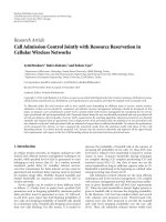
Figure 1: Average number of changes with respect to the number of
locked positions for q
= 16. Only curves with Δω ≥ 0.3 are plotted.
(i) the Lagrange(Q(X), I)procedureoutputsapolyno-
mial L such that L(γ
i
) = Q(γ
i
)foralli ∈ I and
deg(L) <
|I|;
(ii) the GSdecode procedure refers to the Guruswami-
Sudan list decoding (Section 4.3.1). For the sake
of simplicity, we just write GSdecode(Q(X), I)
for the output list of the GS decoding of
(Q(γ
i
0
), ,Q(γ
i
n

−

1
)), i
j
∈{0, , n − 1}\I
with respect to GRS(n
−|I|, k −|I|). So, this
procedure returns a good approximation U(X)of
Q(X), on the evaluation set, of degree less than
k
−|I|;
(iii) the selectposition procedure returns an integer
from the set given as a parameter. This procedure
is used to choose the new position to lock before
retrying list decoding.
Lines 1 to 5 of the algorithm depicted in Algorithm 1 simply
do the setup for the while loop. The while loop, Lines 6 to
12, tries to use list decoding to construct a good solution, as
described above. Remark that if all GS decodings fail, we have
Y
= M −V −L with L is equal to polynomial P of Section 5.1,
that is, we just fall back on Lagrange interpolation. Lines 13
to 16 use the result of the while loop in case of a decoding
success, according to the details given above.
Correctness of this algorithm follows from the fact that
through the whole algorithm we have ev(Y)
·H
t
= m −v·H
t
and Y (γ

i
) = 0fori ∈ I. Termination is clear since each
iteration of the Loop 6-12 increases
|I|.
5.2.2. Algorithm Analysis. The most important property of
embedding algorithms is the number of changes introduced
during the embedding. Let ω(n, k, i) be the average number
of such changes when GRS (n, k)isusedandi positions
are locked. For our algorithm, this quantity depends on two
parameters related to the Guruswami-Sudan algorithm:
EURASIP Journal on Information Security 7
Inputs: v = (v
0
, , v
n−1
), the cover-data
m
= (m
0
, , m
n−k−1
), symbols to hide
I, set of coordinates to remain unchanged,
|I|≤k
Output: s
= (s
0
, , s
n−1
), the stego-data

(s
·H
t
= m; s
i
= v
i
, i ∈ I; d
H
(s, v) ≤ n − k)
(1) V(X)
⇐ v
0
X
0
+ ···+ v
n−1
X
n−1
(2) M(X) ⇐ m
0
X
k
+ ···+ m
n−k−1
X
n−1
(3) L(X) ⇐ Lagrange(M −V, I)
(4) Y(X)
⇐ M(X) −V(X) −L(X)

(5) F(X)
⇐ Lagrange(0, I)
(6) while
|I| <kand GSdecode(
Y
F
, I) = θ do
(7) i
⇐ selectposition({0, , n −1}\I)
(8) I
⇐ I ∪{i}
(9) L(X) ⇐ Lagrange(M −V, I)
(10) F(X)
⇐ Lagrange(0, I)
(11) Y(X)
⇐ M(X) −V(X) −L(X)
(12) end while
(13) if GSdecode(
Y
F
, I)
/
=θ then
(14) U(X)
⇐ GSdecode(
Y
F
, I)
(15) Y(X)
⇐ Y(X) −F(X)U(X)

(16) end if
(17) s
⇐ v +ev(Y)
(18) return s
Algorithm 1: Algorithm for embedding with locked positions using a GRS(n, k)code(γ
0
, , γ
n−1
fixed). It embeds r = n − k F
q
symbols
with up to k locked positions and at most n
−k changes.
(i) the probability p(n, k) that the list decoding of a word
in
F
n
q
outputs a nonempty list of codewords in GRS
(n, k);
(ii) the average distance δ(n, k) between the closest
codewords in the (nonempty) list and the word to
decode.
We deno te by q(n, k) the probability of an empty list and
for conciseness let n

= n −|I|, k

= k −|I|. Thus, the
probability that the first 

− 1 list decodings fail and the th
succeeds can be written as p
∗
()

−1
e=0
q
∗
(e)withp
∗
() =
p(n

−, k

−)andq
∗
(e) = q(n

−e, k

−e). Remark that in
this case, δ
∗
() = δ(n

−, k

−) coordinates are changed on

average.
Now, the average number of changes required to perform
the embedding can be expressed by the following formula:
ω(n, k, i)
=

k

−1

=0
δ
∗
()·p
∗
()
−1

e=0
q
∗
(e)

+(n − k)
k

−1

e=0
q

∗
(e).
(15)
(a) Estimating p and δ. To (upper) estimate p(n, k), we
proceed as follows. Let Z be the random variable equal
to the size of the output list of the decoding algorithm.
The Markov inequality yields Pr(Z
≥ 1) ≤ E(Z), where
E(Z) denotes the expectation of Z.But,Pr(Z ≥ 1) is the
probability that the list is nonempty and, thus, Pr(Z
≥ 1) =
p(n, k). Now, E(Z) is the average number of elements in
the output list, but this is exactly the average number of
0
1
2
3
4
5
6
7
8
9
Average number of modifications
0102030405060
Number of fixed positions
k
= 54
k
= 55

k
= 56
k
= 57
k
= 58
k
= 59
k
= 60
k
= 61
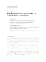
Figure 2: Average number of changes with respect to the number of
locked positions for q
= 64. Only curves with Δω ≥ 0.3 are plotted.
codewords in a Hamming ball of radius λ
GS
. Unfortunately,
no adequate information can be found in the literature
to properly estimate it; the only paper studying a similar
quantity is [25], but it cannot be used for our
E(Z).
8 EURASIP Journal on Information Security
0
2
4
6
8
10
Average number of modifications

0 20 40 60 80 100 120
Number of fixed positions
k
= 116
k
= 118
k
= 119
k
= 120
k
= 121
k
= 122
k
= 123
k
= 124
k
= 125
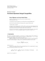
Figure 3: Average number of changes with respect to the number
of locked positions for q
= 128. Only curves with Δω ≥ 0.3are
plotted.
So, we set
E(Z) =
q
k
q
n

·V
λ
GS
=

λ
GS
i=0
(q −1)
i

n
i

q
n−k
, (16)
where V
λ
GS
is the volume of a ball of radius λ
GS
. This would
be the correct value if GRS codes were random codes over
F
q
of length n,withq
k
codewords uniformly drawn from F
n

q
.
That is, we estimate
E(Z)asifGRScodeswererandomcodes.
Thus, we use
p = min(1, q
k−n
V
λ
GS
)toupperestimatep.
The second parameter we need is δ(n, k), the average
number of changes required when the list is nonempty. We
consider that the closest codeword is uniformly distributed
over the ball of radius λ
GS
and, therefore, we have
δ(n, k)
=

λ
GS
i=0
i·(q −1)
i

n
i

V

λ
GS
. (17)
(b) Estimating the Average Number of Changes. Using our
previous estimations for p(n, k)andδ(n, k), we plotted
ω(n, k, i)inFigure 1 (q
= 16), Figure 2 (q = 64), Figure 3
(q
= 128). For each figure, we set n = q −1 and plotted ω for
several values of k.
Remember that i
≤ k and that when i = k,our
algorithm simply uses Lagrange interpolation, which leads to
the maximum number of changes, that is, ω(n, k, k)
= n −k.
On the other side, when i
= 0, our algorithm tries to use
Guruswami-Sudan algorithm as much as possible. Therefore,
our algorithm improves upon the simpler Lagrange interpo-
lation when
Δω
=
ω(n, k, k) −ω(n, k,0)
n −k
(18)
is large. A second criterion to estimate the performance is the
slope of the plotted curves, the slighter, the better.
With this in mind, looking at Figure 1, we can see that
k
= 13 provides good performances; Δω = 0.5, which means

that list decoding avoids up to 50% of the changes required
by Lagrange interpolation, and on the other hand, the slope
is nearly 0 when i
≤ 8. For higher embedding rate, all values
of k less than 3 have Δω
≥ 0.28.
In Figure 2, Δω
≥ 0.3fork ≥ 54. In Figure 3, Δω ≥
0.3fork ≥ 116, except for k = 117. Remark that k = 120,
the slope is nearly 0 for i
≤ 70, which means that we can
lock about half the coordinates and still have Δω
= 42% of
improvement with respect to Lagrange interpolation.
6. Conclusion
We have shown in this paper that Reed-Solomon codes
are good candidates for designing efficient steganographic
schemes. They enable to mix wet papers (locked positions)
and simple syndrome coding (small number of changes) in
order to face not only passive but also active wardens. If
we compare them to the previous studied codes, as binary
BCH codes, Reed-Solomon codes improve the management
of locked positions during embedding, hence ensuring a
better management of the distortion; they are able to lock
twice the number of positions. Moreover, they are optimal
in the sense that they enable to lock the maximal number
of positions. We first provide an efficient way to do it
through Lagrange interpolation. We then propose a new
algorithm based on Guruswami-Sudan list decoding, which
is slower but provides an adaptive tradeoff between the

number of locked positions and the average number of
changes.
In order to use them in real applications, several issues
still have to be addressed. First, we need to choose an
appropriate measure to properly estimate the distortion
induced at the medium level when modifying the symbols
at the data level. Second, we need to use a nonbinary, and
preferably large, alphabet. A straightforward way to deal with
this would be to simply regroup bits to obtain symbols of
our alphabet and consider that a symbol should be locked
if it contains a bit that should be. Unfortunately, it would
lead to a large number of locked symbols (e.g., 5% of locked
bits leads to up to 20% of locked symbols if we use GF(16)).
A better way would be to use grid coloring [26], keeping
a 1-to-1 ratio. But, the price to this 1-to-1 ratio would be
a cut in payload. We think a good solution has yet to be
figured out. Nevertheless, in some settings, a large alphabet
arises naturally; for example, in [14], a (binary) wet paper
code is used on the syndromes of a [2
k
− 1, 2
k
− k − 1]
Hamming code, some of these syndromes being locked; here,
since whole syndromes are locked, we can view syndromes
as elements of the larger field GF(2
k
) and use our proposal.
Third, no efficient implementation of the Guruswami-Sudan
list decoding algorithm is available. And, as the involved

mathematical problems are really tricky, only a specialist can
perform a real efficient one. Today, these three issues remain
open.
EURASIP Journal on Information Security 9
Appendix
Guruswami-Sudan Algorithm
We provide here the core of the Guruswami-Sudan algo-
rithm, without deep details on (important) algorithms that
are required to achieve a good complexity (the interested
reader may refer to [19, 24, 25]).
A.1. Des cription. Recall we have a vector ev(Q)
= (Q(γ
0
),
, Q(γ
n−1
)) and we want to find all polynomials P such that
ev(P) is at distance at most λ from ev(Q), and deg(P) <k.
We construct a bivariate polynomial R over
F
q
such that
R(γ
i
, P(γ
i
)) = 0forallP at distance at most λ from Q.Then,
we compute all P from a factorization of R.
First, let us define what is called the multiplicity of a
zero for bivariate polynomial: R(X, Y)hasazero(a, b)of

multiplicity μ if and only if the coefficients of the monomials
X
i
Y
j
in R(X +a, Y +b)areequaltozeroforalli, j with i+ j<
μ.Thisleadsto

μ+1
2

linear equations in the coefficients of
R. Writing R(X, Y)
=

i,j
r
i,j
X
i
Y
j
, then R(X + a, Y + b) =

i,j
r
i,j
(a, b)X
i
Y

j
with
r
i,j
(a, b) =

i

≥i
j

≥j

i

i

j

j

r
i

,j

a
i

−i

b
j

−j
. (A.1)
Since a multiplicity μ in (a, b)isexactlyr
i,j
(a, b) = 0fori+j<
μ,andwehave

μ+1
2

values of i and j such that i + j<μ,we
have the right number of equations.
The principle is to use the n

μ+1
2

linear equations in the
coefficients of R, obtained by requiring (γ
i
, Q(γ
i
)) to be a zero
of R with multiplicity μ for i
∈{0, , n − 1}. Solving this
system leads to the bivariate polynomial R,but,tobesure
our system has a solution, we need more unknowns than

equations. To address this point, we impose a special shape
on R. For a fixed integer ,wesetR(X, Y)
=

j≤
R
j
(X)Y
j
with the restriction that deg(R
j
) ≤ μ(n −λ)− j(k −1). Thus,
R has at most

j≤l
deg(R
j
) = ( +1)μ(n −λ) −
( +1)
2
(k
−1) (A.2)
coefficients. Choosing  such that

j≤
deg(R
j
) >n

μ+1

2

guarantees to have nonzero solutions. Of course, since
degrees of R
j
must be nonnegative integers, we have λ ≤
n −(/μ)(k −1).
On the other hand, under the conditions we imposed on
R, one can prove that for all polynomials P of degree less than
k and at distance at most λ from Q, Y
−P(X)dividesR(X, Y).
Detailed analysis of the parameters shows it is always possible
to take  less than or equal to

≤

k
(k −1)
2
n(μ +1)μ (A.3)
(see [19, Chapter 5]). Thus, we have the formula λ
≈ n −1 −


n(k −1)(1 + (1/μ)), which leads to the maximum radius
λ
GS
= max
μ≥1
λ = n −1 −


n(k −1) for μ large enough.
A.2. Complexity. Using 
= m
√
n/k in (A.2), there are n

μ
2

linear equations with roughly nμ
2
unknowns. Solving these
equations with fast general linear algebra can be done in
less than O(n
5/2
μ
5
) arithmetic operations over F
q
(see [27,
Chapter 12]).
Finding the factor Y
− P(X) can be achieved in a
simple way, considering an extension of
F
q
of order k.A
(univariate) polynomial P over
F

q
of degree less than k can be
uniquely represented by an element

P of F
q
k
and, under this
representation, to find factors Y
−P(X)ofR is equivalent to
find factors Y
−

P of

R(Y) =

j≤l

R
j
Y
j
, that is, to compute
factorization of a univariate polynomial of degree  over
F
q
k
which can be done in at most O(μ·
√

n·k
3
)operationsover
F
q
, neglecting logarithmic factors (see [27, Chapter 14]).
The global cost of this basic approach is heavily dom-
inated by the linear algebra part in O(n
5/2
μ
5
)witha
particularly large degree in μ. It is possible to perform
the Guruswami-Sudan algorithm at a cheaper cost, still in
O(n
2
μ
4
), with less naive algorithms. Complete details can be
found in [25].
To sum up, Guruswami-Sudan decoding algorithm finds
polynomials P of degree at most k and at distance at most
n
− 1 −

n(k −1) from Q using simple linear algebra and
factorization of univariate polynomial over a finite field for a
cost in less than O(n
5/2
μ

5
) arithmetic operations in F
q
. This
can be reduced to O(n
2
μ
4
) with dedicated algorithms.
Acknowledgments
Dr. C. Fontaine is supported (in part) by the European
Commission through the IST Programme under Contract
IST-2002-507932 ECRYPT and by the French National
Agency for Research under Contract ANR-RIAM ESTIVALE.
TheauthorsareindebttoDanielAugotfornumerous
comments on this work, in particular for pointing out the
adaptation of the Guruswami-Sudan algorithm to shortened
GRS used in the embedding algorithm.
References
[1] G. J. Simmons, “The prisoners’ problem and the subliminal
channel,” in Advances in Cryptology, pp. 51–67, Plenum Press,
New York, NY, USA, 1984.
[2] R. B
¨
ohme and A. Westfeld, “Exploiting preserved statistics for
steganalysis,” in Proceedings of the 6th International Workshop
on Information Hiding (IH ’04), vol. 3200 of Lecture Notes in
Computer Science, pp. 82–96, Springer, Toronto, Canada, May
2004.
[3] E. Franz, “Steganography preserving statistical properties,” in

Proceedings of the 5th International Workshop on Information
Hiding (IH ’02), vol. 2578 of Lecture Notes in Computer Science,
pp. 278–294, Noordwijkerhout, The Netherlands, October
2002.
[4] R. Crandall, Some notes on steganography. Posted on
steganography mailing list, 1998, />∼westfeld/crandall.pdf.
[5] J. Bierbrauer, On Crandall’s problem. Personal communica-
tion, 1998, />.pdf.
10 EURASIP Journal on Information Security
[6] A. Westfeld, “F5—a steganographic algorithm: high capacity
despite better steganalysis,” in Proceedings of the 4th Interna-
tional Workshop on Information Hiding (IH ’01), vol. 2137 of
Lecture Notes in Computer Science, pp. 289–302, Pittsburgh, Pa,
USA, April 2001.
[7] F. Galand and G. Kabatiansky, “Information hiding by cov-
erings,” in Proceedings of IEEE Information Theory Workshop
(ITW ’03), pp. 151–154, Paris, France, March-April 2003.
[8] J. Fridrich, M. Goljan, P. Lisonek, and D. Soukal, “Writing on
wet paper,” IEEE Transactions on Signal Processing, vol. 53, no.
10, part 2, pp. 3923–3935, 2005.
[9] J. Fridrich, M. Goljan, and D. Soukal, “Efficient wet paper
codes,” in Proceedings of the 7th International Workshop on
Information Hiding (IH ’05), vol. 3727 of Lecture Notes in
Computer Science, pp. 204–218, Barcelona, Spain, June 2005.
[10] J. Fridrich, M. Goljan, and D. Soukal, “Wet paper codes
with improved embedding efficiency,” IEEE Transactions on
Information Forensics and Security, vol. 1, no. 1, pp. 102–110,
2006.
[11] J. Fridrich and D. Soukal, “Matrix embedding for large
payloads,” IEEE Transactions on Information Forensics and

Securit y, vol. 1, no. 3, pp. 390–395, 2006.
[12] D. Sch
¨
onfeld and A. Winkler, “Embedding with syndrome
coding based on BCH codes,” in Proceedings of the 8th
Workshop on Multimedia and Security (MM&Sec ’06), pp. 214–
223, ACM, Geneva, Switzerland, September 2006.
[13] D. Sch
¨
onfeld and A. Winkler, “Reducing the complexity of
syndrome coding for embedding,” in Proceedings of the 9th
International Workshop on Information Hiding (IH ’07), vol.
4567 of Lecture Notes in Computer Science, pp. 145–158,
Springer, Saint Malo, France, June 2007.
[14] W. Zhang, X. Zhang, and S. Wang, “Maximizing stegano-
graphic embedding efficiency by combining Hamming codes
and wet paper codes,” in Proceedings of the 10th International
Workshop on Information Hiding (IH ’08), vol. 5284 of Lecture
Notes in Computer Science, pp. 60–71, Santa Barbara, Calif,
USA, May 2008.
[15] J. Bierbrauer and J. Fridrich, “Constructing good covering
codes for applications in steganography,” in Transactions
on Data Hiding and Multimedia Security III, vol. 4920 of
Lecture Notes in Computer Science, pp. 1–22, Springer, Berlin,
Germany, 2008.
[16] J. Fridrich, M. Goljan, and D. Soukal, “Perturbed quantization
steganography,” ACM Multimedia and Security Journal, vol. 11,
no. 2, pp. 98–107, 2005.
[17] A. Vardy, “The intractability of computing the minimum
distance of a code,” IEEE Transactions on Information Theory,

vol. 43, no. 6, pp. 1757–1766, 1997.
[18] A. McLoughlin, “The complexity of computing the covering
radius of a code,” IEEE Transactions on Information Theory,
vol. 30, no. 6, pp. 800–804, 1984.
[19] W. C. Huffman and V. Pless, Fundamentals of Error-Correcting
Codes, Cambridge University Press, Cambridge, UK, 2003.
[20] Y. Kim, Z. Duric, and D. Richards, “Modified matrix encoding
technique for minimal distortion steganography,” in Proceed-
ings of the 8th International Workshop on Information Hiding
(IH ’06), vol. 4437 of Lecture Notes in Computer Science,pp.
314–327, Springe, Alexandria, Va, USA, June 2006.
[21] F. Galand and G. Kabatiansky, “Steganography via covering
codes,” in Proceedings of the IEEE International Symposium on
Information Theory (ISIT ’03), p. 192, Yokohama, Japan, June-
July 2003.
[22] X. Zhang and S. Wang, “Stego-encoding with error correction
capability,” IEICE Transactions on Fundamentals of Electronics,
Communications and Computer Sciences, vol. E88-A, no. 12,
pp. 3663–3667, 2005.
[23] M. Sudan, “Decoding of Reed Solomon codes beyond the
error-correction bound,” Journal of Complexity, vol. 13, no. 1,
pp. 180–193, 1997.
[24] V. Guruswami and M. Sudan, “Improved decoding of Reed-
Solomon and algebraic-geometry codes,” IEEE Transactions on
Information Theory, vol. 45, no. 6, pp. 1757–1767, 1999.
[25] R. J. McEliece, “The Guruswami-Sudan decoding algorithm
for Reed-Solomon codes,” IPN Progress Report 42-153,
California Institute of Technology, Pasadena, Calif, USA, May
2003, />report/42-153/153F
.pdf.

[26] J. Fridrich and P. Lisonek, “Grid colorings in steganography,”
IEEE Transactions on Information Theory,vol.53,no.4,pp.
1547–1549, 2007.
[27] J. von zur Gathen and J. Gerhard, Modern Computer Algebra,
Cambridge University Press, Cambridge, UK, 2nd edition,
2003.