Báo cáo hóa học: " Research Article On the Impact of Entropy Estimation on Transcriptional Regulatory Network Inference Based on Mutual Information" potx

Hindawi Publishing Corporation
EURASIP Journal on Bioinformatics and Systems Biology
Volume 2009, Article ID 308959, 9 pages
doi:10.1155/2009/308959
Research Article
On the Impact of Entropy Estimation on Transcriptional
Regulatory Network Inference Based on Mutual Information
Catharina Olsen, Patrick E. Meyer, and Gianluca Bontempi
Machine Learning Group, Computer Science D epartme nt, Faculty of Scie nce, Universit
´
e Libre de Bruxelles,
CP 212, 1050 Brussels, Belgium
Correspondence should be addressed to Catharina Olsen,
Received 31 May 2008; Accepted 8 October 2008
Recommended by Dirk Repsilber
The reverse engineering of transcription regulatory networks from expression data is gaining large interest in the bioinformatics
community. An important family of inference techniques is represented by algorithms based on information theoretic measures
which rely on the computation of pairwise mutual information. This paper aims to study the impact of the entropy estimator
on the quality of the inferred networks. This is done by means of a comprehensive study which takes into consideration three
state-of-the-art mutual information algorithms: ARACNE, CLR, and MRNET. Two different setups are considered in this work.
The first one considers a set of 12 synthetically generated datasets to compare 8 different entropy estimators and three network
inference algorithms. The two methods emerging as the most accurate ones from the first set of experiments are the MRNET
method combined with the newly applied Spearman correlation and the CLR method combined with the Pearson correlation.
The validation of these two techniques is then carried out on a set of 10 public domain microarray datasets measuring the
transcriptional regulatory activity in the yeast organism.
Copyright © 2009 Catharina Olsen et al. This is an open access article distributed under the Creative Commons Attribution
License, which permits unrestricted use, distribution, and reproduction in any medium, provided the original work is properly
cited.
1. Introduction
The inference of regulatory networks by modeling depen-
dencies at the transcription level aims at providing biologists

with an additional insight about cell activities. This task
belongs to the domain of systems biology which studies the
interactions between the components of biological systems
and how these interactions give rise to the function and the
behavior of the whole system. This approach differs from
the so-called “reductionist approach” that limits its focus to
the building blocks of the system without providing a global
picture of the cell behavior, as stated in [1]:
“the reductionist approach has successfully
identified most of the components and many
of the interactions but, unfortunately, offers no
convincing concepts or methods to understand
how system properties emerg the pluralism of
causes and effects in biological networks is better
addressed by observing, through quantitative
measures, multiple components simultaneously
and by rigorous data integration with mathe-
matical models.”
The reverse engineering of transcriptional regulatory
networks (TRNs) from expression data is known to be a
very challenging task because of the large amount of noise
intrinsic to the microarray technology, the high dimension-
ality, and the combinatorial nature of the problem. Also, a
gene-to-gene network inferred on the basis of transcriptional
measurements returns only a rough approximation of a com-
plete biochemical regulatory network since many physical
connections between macromolecules might be hidden by
shortcuts. Notwithstanding, in recent years, computational
techniques have been applied with success to this domain,
as witnessed by successful validations of the interaction

networks predicted by the algorithms [2].
Network inference consists in representing the stochastic
dependencies between the variables of a dataset by means
of a graph. Mutual information networks are an important
category of network inference methods.
2 EURASIP Journal on Bioinformatics and Systems Biology
Information-theoretic approaches typically rely on the
estimation of mutual information (MI) from expression
data in order to measure the statistical dependence between
genes [3]. In these methods, a link between two nodes is
established if it exhibits a significant score estimated by
mutual information. The role of the mutual information
estimator is therefore essential to guarantee a high accuracy
rate. Notwithstanding, few experimental studies about the
impact of the estimator on the quality of the inferred network
exist [4]. To the best of our knowledge, this paper presents
the first comprehensive experimental comparison of several
mutual information estimation techniques and state-of-the-
art inference methods like MRNET [3], ARACNE [5], and
CLR [6]. An additional contribution of this paper is the study
of the impact of the correlation estimator (notably Spearman
and Pearson) on the mutual information computation once
a hypothesis of normality is done. Interestingly enough, the
Spearman- and the Pearson-based information estimators
emerge as the most competitive techniques once combined
with the MRNET and the CLR inference strategies, respec-
tively.
The first part of the experimental session aims at studying
the sensitivity to noise and missing values of different
discretization, estimation, and network inference methods.

For this purpose, a synthetic benchmark is created by means
of the SynTReN data generator [7].
In the second part, the techniques which appeared to
be the most effective in the synthetic session are assessed
by means of a biological microarray benchmark which
integrates several public domain yeast microarray datasets.
The outline of the paper is as follows. Section 2
reviews the most important mutual information estimators.
Section 3 introduces some state-of-the-art network inference
algorithms. Section 4 contains the description of the syn-
thetic data generator, the description of the real data setting,
and the related discussions of the results. Section 5 concludes
the paper.
2. Estimators of Information
An information theoretic network inference technique aims
at identifying connections between two genes (variables)
by estimating the amount of information between them.
Different information measures exist in the literature [8]. In
this article, we focus on the mutual information measure and
the related estimation techniques. Note that, if the estimation
technique has been conceived for discrete random variables,
a discretization procedure has to be executed before applying
the estimation procedure to expression data.
2.1. Mutual Information. Mutual information is a well-
known measure which quantifies the stochastic dependency
between two random variables without making any assump-
tion (e.g., linearity) about the nature of the relation [9].
Let X be a discrete random vector whose ith component
takes values in the discrete set X
i

of size |X
i
|. The (i, j)th
element of the mutual information matrix (MIM) associated
to X is defined by
MIM
ij
= H

X
i

+ H

X
j

−
H

X
i
, X
j

=
I

X
i

; X
j

=

k
i
∈X
i

k
j
∈X
j
p

x
k
i
, x
k
j

log

p

x
k
i

, x
k
j

p

x
k
i

p

x
k
j


,
(1)
where the entropy of a discrete random variable X
i
is defined
as
H

X
i

=−


k
i
∈X
i
p

x
k
i

log p

x
k
i

,(2)
and I(X
i
; X
j
) is the mutual information between the random
variables X
i
and X
j
.
2.2. Entropy Estimation. In practical setups, the underlying
distribution p of the variables is unknown. Consequently,
the entropy terms in (1) cannot be computed directly but

require an estimation. Many different approaches to entropy
estimation have been introduced. In this paper, we restrict
the choice to the following five estimators: empirical, Miller-
Madow, shrink, Pearson and Spearman correlation.
2.2.1. Empirical. Let X be a continuous random variable
taking values in the real interval [a, b]. Suppose the interval
is partitioned into
|X| bins, where X denotes the bin index
vector, nb(x
k
) denotes the number of data points in the kth
bin, and m
=

k∈X
nb(x
k
) stands for the total number of
observations.
The empirical estimator, also known as the maximum
likelihood estimator, is the entropy of the empirical distribu-
tion

H
emp
=−

k∈X
nb


x
k

m
log
nb

x
k

m
. (3)
It has been shown in [10] that the asymptotic bias of this
estimator amounts to
bias


H
emp

=−
|
X|−1
2m
. (4)
2.2.2. Miller-Madow. The Miller-Madow estimator [10]
corrects the biased empirical estimator by removing the
estimatedbiastermfromit(4):

H

mm
=

H
emp
+
|X|−1
2m
. (5)
This estimator reduces the bias of (3) without increasing its
variance.
2.2.3. Shrink. The shrink estimator [8] combines two differ-
ent estimators, one with low variance and one with low bias,
by using the weighting factor λ
∈ [0, 1]:

p
λ

x
k

=
λ
1
|X|
+(1−λ)
nb

x

k

m
. (6)
EURASIP Journal on Bioinformatics and Systems Biology 3
Let
λ
∗
= arg min
λ∈[0,1]
E
⎡
⎣

k∈X


p
λ

x
k

− p

x
k

2
⎤

⎦
(7)
be the value minimizing the mean square function [8]. It has
been shown in [11] that the optimal λ is given by
λ
∗
=
|
X|

m
2
−

k∈X
nb

x
k

2

(m − 1)

|
X|

k∈X
nb


x
k

2
− m
2

. (8)
2.2.4. Pearson Correlation. Correlation is a statistic measur-
ing the strength and the direction of the linear relationship
between two random variables. The Pearson correlation
between two random variables X and Y is defined as
ρ
=
cov(X,Y)
σ
X
σ
Y
. (9)
Correlation takes values in [
−1, 1], where |ρ|=1denotesa
linear relation between the variables X and Y. If the variables
are independent, the correlation is equal to zero while the
opposite is not necessarily true (e.g., nonlinear dependency).
It can be shown that correlation and mutual information
are related if the joint distribution is normal.
Let
f (X)
=

1

(2π)
n
|C|
exp
(−(1/2)(x−μ)
T
C
−1
(x−μ))
(10)
be the density of a multivariate Gaussian variable X with
mean μ and covariance matrix C. The entropy of this
distribution is given by
H(X)
=
1
2
ln

(2πe)
n
|C|

, (11)
where
|C| is the determinant of the covariance matrix [12].
The mutual information between two variables X
i

and X
j
is
then given by
I

X
i
, X
j

=
1
2
log

σ
ii
σ
jj
|C|

(12)
=−
1
2
log

1 − ρ
2


,
(13)
where ρ is the Pearson’s correlation.
Since the functional relation (13) between the mutual
information and the correlation is a monotone function, it
is sufficient to use ρ
2
when computing this value.
The Pearson correlation can be estimated from the
measurements x
i
and y
i
of two genes X and Y by the
following equation:
ρ =

m
i
=1
x
i
y
i
−

m
i
=1

x
i

m
i
=1
y
i

n

m
i=1
x
2
i
−


m
i=1
x
i

2

n

m
i=1

y
2
i
−


m
i=1
y
i

2
. (14)
2.2.5. Spearman Correlation. The Spearman rank correlation
coefficient is a special case of the Pearson correlation in which
the data are converted to rankings before calculating the
coefficient.
The Spearman correlation can be calculated using (14),
where the terms x
i
and y
i
are replaced by their respective
ranks. Note that the Spearman rank correlation coefficient
generalizes the Pearson correlation coefficient by being able
to detect not only linear relationships between the variables
but also any kind of monotone relation without making any
assumptions about the distributions of the variables.
2.3. Discretization Methods. The mutual information esti-
mators in Sections 2.2.1, 2.2.2,and2.2.3 apply to discrete

random variables. In order to use them for continuous
random variables, a discretization step is required. The two
most widely used methods for discretization are the equal
width and the equal frequency methods [13].
Equal Width. This discretization method partitions the
domain of X into
|X| subintervals of equal size. As a
consequence, the number of data points in each bin is likely
to be different.
Equal Frequency. This method divides the interval [a, b] into
|X| subintervals, each containing the same number of data
points. It follows that subinterval sizes are typically different.
The number of subintervals should be chosen so that all
bins contain a significant number of samples. In [14], the
authors propose to use
|X|=
√
m,wherem is the total
number of samples.
3. Network Inference Algorithms
The network inference proceeds in two steps. In the first
step, the mutual information matrix is calculated. In the
second step, the chosen algorithm is applied to the mutual
information matrix in order to compute a score that is used
to weigh the links between network nodes.
3.1. The MRNET Method. The MRNET method [3]isbased
on the maximum relevance/minimum redundancy (MRMR)
feature selection technique [15]. This iterative selection
technique chooses at each step, among the least redundant
variables, the one having the highest mutual information

with the target.
The method ranks the set of inputs according to a score
which is the difference between the mutual information with
the output variable Y (maximum relevance) and the average
mutual information with the previously ranked variables
(minimum redundancy). The network is inferred by deleting
all edges whose score lies below a given threshold.
Direct interactions should be well ranked whereas indi-
rect interactions should be badly ranked. In the first step,
variable X
i
which has the highest mutual information to the
target Y is selected. The second selected variable X
j
will be
the one with a high information I(X
j
; Y) to the target and at
the same time a low information I(X
j
; X
i
) to the previously
selected variable.
4 EURASIP Journal on Bioinformatics and Systems Biology
In the next steps, given a set X
S
of selected variables, the
criterion updates X
S

by choosing the variable that maximizes
the score
s
j
= I

X
j
; Y

−
1
|S|

X
k
∈X
S
I

X
j
; X
k

, (15)
which can be described as a relevance term minus a
redundancy term.
For each pair
{X

i
, X
j
}, the algorithm returns two scores
s
i
and s
j
and computes the maximum of the two. All edges
with a score below a given threshold are then deleted.
3.2. The ARACNE Method. The algorithm for the recon-
struction of accurate cellular networks (ARACNEs) [5]is
based on the data processing inequality [16]. This inequality
states that if the interaction between X
1
and X
3
depends on
X
2
, then
I

X
1
; X
3

≤
min


I

X
1
; X
2

, I

X
2
; X
3

. (16)
The algorithm assigns a weight to each pair of nodes which is
equal to the mutual information between the variables. Then,
the minimal mutual information between three variables is
computed, and eventually the edge with the lowest value is
interpreted as an indirect connection and removed if the
difference between the two lowest weights is above a given
threshold.
3.3. The CLR Method. In the context likelihood or relat-
edness (CLR) algorithm [6], the mutual information is
calculated for each pair of variables. Then, a score related to
the empirical distribution of these MI values is computed. In
particular, instead of considering the information I(X
i
; X

j
)
between two variables X
i
and X
j
, the algorithm takes into
account the score z
ij
=

z
2
i
+ z
2
j
,where
z
i
= max

0,
I

X
i
; X
j


− 
μ
i
σ
i

, (17)
and
μ
i
and σ
i
are, respectively, the mean and the standard
deviations of the empirical distribution of the mutual
information values I(X
i
, X
k
), k = 1, , n.
4. Experiments
This section contains two parts. In the first part, several
inference methods and estimators are applied to synthetic
datasets with different noise and missing values configura-
tions. The aim of this part is to identify the best combination
of estimator and inference method. Once the assessment
on the synthetic benchmark is done, the best performing
techniques are then applied to a biological problem. The
aim of this second experiment is to assess the capability
of the algorithms of discovering interactions of the yeast
transcriptome uniquely on the basis of expression data.

All computations were carried out using the R-pack-
age MINET [17]( />minet). This recently introduced package allows the use of
three different inference methods, namely, ARACNE [5],
CLR [6], and MRNET [3].
The following entropy estimators are also made available
to calculate the mutual information: empirical, Miller-
Madow, shrink, and Pearson correlation.
Note that, in order to apply the first three estimators
to expression data, two different discretization methods are
implemented: equal frequency and equal width discretiza-
tion with default size
|X|=
√
m.
4.1. Synthetic Data
4.1.1. Network Generation. The synthetic benchmark relies
on several artificial microarray datasets generated by the
SynTReN generator [7]. This simulator emulates the gene
expression process by adopting topologies derived from
subnetworks of E.coli and S.cerevisiae networks. Interaction
kinetics are modeled by nonlinear differential equations
based on Michaelis-Menten and Hill kinetics.
We used the SynTReN generator to create twelve bench-
mark datasets whose number m of samples and number n of
genes are detailed in Tab le 1.
4.1.2. Introducing Missing Values. In order to study the
impact of missing values, expression values were removed
from the generated datasets. The number of missing values
is distributed according to the β(a, b) distribution with
parameters a

= 2andb = 5. The maximal allowed
number of missing values is a third of the entire dataset. This
distribution was utilized, instead of the uniform distribution,
because the latter one could have favored the empirical
estimator.
4.1.3. Setup. For each experiment, ten repetitions were
carried out. Each dataset was analyzed using three infer-
ence methods (i.e., MRNET, ARACNE, and CLR) and the
following estimators: Pearson correlation, empirical, Miller-
Madow, shrink, and the Spearman correlation coefficient.
The empirical, the Miller-Madow, and the shrink estimator
were computed applying the equal width and the equal
frequency discretization approaches. Furthermore, the com-
putation was carried out with and without additive Gaussian
noise (having 50% variance of the observed values). Each
of these setups was also assessed with introduced missing
values.
4.1.4. Validation. Network inference algorithms infer either
the presence or the absence of an edge for each pair of nodes.
Similarly to classification, we define the possible outcomes
of inference as follows. A true positive (TP) occurs when an
edge is correctly predicted as existing, a false positive (FP)
occurs when a nonexisting edge is inferred, true negative
(TN) occurs when a nonexisting edge is not inferred, and
false negative (FN) occurs when an existing edge is not
detected.
EURASIP Journal on Bioinformatics and Systems Biology 5
Table 1: Generated datasets. Number of genes n, number of
samples m.
No. Dataset Source net nm

1 ecoli 300 300 E.coli 300 300
2 ecoli
300 200 E.coli 300 200
3 ecoli
300 100 E.coli 300 100
4 ecoli
300 50 E.coli 300 50
5 ecoli 200 300 E.coli 200 300
6 ecoli
200 200 E.coli 200 200
7 ecoli
200 100 E.coli 200 100
8 ecoli
200 50 E.coli 200 50
9 ecoli 100 300 E.coli 100 300
10 ecoli
100 200 E.coli 100 200
11 ecoli
100 100 E.coli 100 100
12 ecoli
100 50 E.coli 100 50
Once the numbers of TP, FP, TN, and FN are computed,
we can measure precision and recall
p
=
TP
TP + FP
,
r
=

TP
TP + FN
.
(18)
Precision measures the fraction of real edges among the ones
classified as positive while recall quantifies the fraction of real
edges that are correctly inferred.
A weighted harmonic average of precision and recall is
returned by the F-score [18]:
F
=
2pr
r + p
∈ [0, 1], (19)
which attains its maximum value 1 when the returned
network is without any error.
To validate the simulation’s results, the maximal F-score
was computed for each experiment. Using a paired t-test,
the maximal F-scores were then compared and statistically
validated.
4.1.5. Discussion of Results. The results of the synthetic
benchmark are collected in Ta bl e 2 which returns the F-
score for each combination of inference method, mutual
information estimator, and nature of the dataset (noisy
versus not noisy, complete versus missing data). Note that the
maximal F-score is highlighted together with the F-scores
which are not significantly different from the best.
We analyze the results according to four different aspects:
the impact of the estimator, the impact of the discretization,
the impact of the inference algorithm, and the influence of

sample and network size.
The section concludes with the identification of the best
combination of inference algorithm and estimator.
Impact of the Estimator. In case of complete datasets with
no noise, the empirical and the Miller-Madow estimators
with equal-frequency binning lead to the highest F-scores
for the MRNET and the ARACNE inference methods. The
Spearman correlation is not significantly different from the
best, in case of ARACNE, and is close to the best in case of
MRNET. The CLR method is less sensitive to the estimator,
and the best result is obtained with the Pearson correlation.
In case of noisy data or missing value (NA) configura-
tions, the Pearson correlation and the Spearman correlation
lead to the highest F-score for all inference methods. A slight
better accuracy of the Pearson correlation can be observed
in presence of missing values. The Spearman correlation
outperforms the other estimators in MRNET and ARACNE
when complete yet noisy datasets are considered. In CLR,
Pearson and Spearman correlations lead the ranking without
being significantly different.
Impact of the Discretization. In case of complete datasets with
no noise, the equal frequency binning approach outperforms
the equal width binning approach for all discrete estimators.
The gap between the two discretization methods is clearly
evident in MRNET and less striking in ARACNE and CLR.
In case of noisy or missing data configurations, differences
are attenuated.
Impact of the Inference Algorithm. In case of complete
datasets with no noise, the MRNET inference technique
outperforms the other algorithms.

The situation changes in presence of noisy or missing
values. Here, CLR appears to be the most robust by returning
the highest F-scores for all combinations of noise and
missing values.
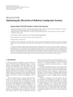
Impact of Number of Sample and N etwork Sizes. The role
of network size is illustrated in Figure 1 (first row) which
shows how the F-score decreases as long as the network size
increases. This behavior can be explained by the increasing
difficulty of recovering a larger underlying network in front
of an increasing dimensionality of the modeling task.
In Figure 1 (second row), the values of the F-score seem
not to be influenced substantially by the number of samples.
Conclusion. A concise summary of the previously discussed
results is displayed in Ta b le 3 which averages the accuracy
over the different data configurations.
It emerges that the most promising combinations are
represented by the MRNET algorithm with the Spearman
estimator and the CLR algorithm with the Pearson correla-
tion. The former seems to be less biased because of its good
performance in front of nonnoisy datasets while the latter
seems to be more robust since it is less variant in front of
additive noise.
4.2. Biological Data. The second part of the experimental
session aims to assess the performance of the two selected
techniques once applied to a real biological task.
We proceeded by (i) setting up a dataset which combines
several public domain microarray datasets about the yeast
transcriptome activity, (ii) carrying out the inference with
6 EURASIP Journal on Bioinformatics and Systems Biology
300200100

Number of genes
0
0.1
0.2
0.3
0.4
F-score
30020010050
Number of samples
0
0.1
0.2
0.3
0.4
F-score
(a)
300200100
Number of genes
0
0.1
0.2
0.3
0.4
F-score
30020010050
Number of samples
0
0.1
0.2
0.3

0.4
F-score
(b)
300200100
Number of genes
0
0.1
0.2
0.3
0.4
F-score
30020010050
Number of samples
0
0.1
0.2
0.3
0.4
F-score
(c)
Figure 1: (First row) Mean F-scores and standard deviation with respect to number of genes. (Second row) Mean F-scores and standard
deviation with respect to number of samples. For all, 10 repetitions with additive Gaussian noise of 50% with full datasets (no missing
values). Inference methods: (a) MRNET, (b) ARACNE, and (c) CLR.
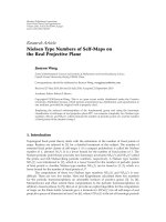
10.80.60.40.20
FPR
Harbison
CLR with Pearson correlation
MRNET with Spearman correlation
CLR with Miller-Madow, equal frequency
MRNET with Miller-Madow, equal frequency

Random
0
0.2
0.4
0.6
0.8
1
TPR
Figure 2: ROC curves: Harbison network, CLR combined with
Pearson correlation, MRNET with Spearman correlation, CLR
combined with the Miller-Madow estimator using the equal fre-
quency discretization method, MRNET with Miller-Madow using
equal frequency discretization and random decision.
the two selected techniques, and (iii) assessing the quality
of the inferred network with respect to two independent
sources of information: the list of interactions measured
by means of an alternative genomic technology and a list
of biologically known gene interactions derived from the
TRANSFAC database.
4.2.1. The Datas et. The dataset was built by first normal-
izing and then joining ten public domain yeast microarray
datasets, whose number of samples and origin is detailed in
Ta bl e 4. The resulting dataset contains the expression of 6352
yeast genes in 711 experimental conditions.
4.2.2. Assessment by ChIP-Chip Technology. The first vali-
dation of the network inference outcome is obtained by
comparing the inferred interactions with the outcome of a
set of ChIP-chip experiments. The ChIP-chip technology,
detailed in [28], measures the interactions between proteins
and DNA by identifying the binding sites of DNA-binding

proteins. The procedure can be summarized as follows. First,
the protein of interest is cross-linked with the DNA site it
binds to, then double-stranded parts of DNA fragments are
extracted. The ones which were cross-linked to the protein of
interest are filtered out from this set and reverse cross-linked.
Also, their DNA is purified. In the last step, the fragments
are analyzed using a DNA microarray in order to identify
gene-gene connections. For our purposes, it is interesting to
remark that the ChIp-chip technology returns for each pair
of genes a probability of interaction. In particular we use,
for the validation of our inference procedures, the ChIp-chip
measures of the yeast transcriptome provided in [29].
4.2.3. Assessment by Biological Knowledge. The second vali-
dation of the network inference outcome relies on existing
biological knowledge and in particular on the list of putative
interactions in Saccharomyces cerevisiae published in [30].
EURASIP Journal on Bioinformatics and Systems Biology 7
Table 2: MINET results: noise stands for Gaussian additive noise,
NA for missing values, eqf for equal frequency, and eqw for
equal width. In bold face maximum F-scores and significantly not
different values.
Method MRnet
Estimator
No noise,
no NA
Noise,
no NA
No noise,
NA
Noise,

NA
Pearson
0.2006 0.1691 0.1790 0.1611
Spearman
0.3230 0.1771 0.1464 0.1333
Emp eqf
0.3420 0.1551 0.1136 0.0868
Emp eqw
0.2028 0.1650 0.1036 0.0822
MM eqf
0.3396 0.1524 0.1140 0.0924
MM eqw
0.1909 0.1592 0.1068 0.0883
Shr eqf
0.3306 0.1506 0.1150 0.0788
Shr eqw
0.1935 0.1574 0.1090 0.0839
Aracne
Pearson
0.1117 0.1082 0.1054 0.1069
Spearman
0.1767 0.1156 0.1167 0.1074
Emp eqf
0.1781 0.1042 0.0993 0.0765
Emp eqw
0.1287 0.1082 0.0892 0.0727
MM eqf
0.1786 0.1032 0.0985 0.0783
MM eqw
0.1217 0.1049 0.0931 0.0767

Shr eqf
0.1736 0.1000 0.1009 0.0697
Shr eqw
0.1152 0.1045 0.0898 0.0717
CLR
Pearson
0.2242 0.1941 0.2231 0.1911
Spearman
0.2197 0.1915 0.1806 0.1582
Emp eqf
0.2123 0.1729 0.1847 0.1397
Emp eqw
0.2098 0.1724 0.1799 0.1327
MM eqf
0.2128 0.1729 0.1860 0.1427
MM eqw
0.2083 0.1723 0.1845 0.1384
Shr eqf
0.2096 0.1670 0.1864 0.1311
Shr eqw
0.2030 0.1659 0.1822 0.1333
Table 3: For each method and estimator, the mean over the four
different setups: no NA, no noise; no NA, noise; NA, no noise; NA
noise. In bold face the best mean F-score.
Estimator Method
MRnet Aracne CLR
Pearson 0.1775 0.1081 0.2081
Spearman 0.1950 0.1285 0.1863
Emp eqf 0.1744 0.1145 0.1774
Emp eqw 0.1384 0.0997 0.1737

MM eqf 0.1746 0.1147 0.1786
MM eqw 0.1363 0.0881 0.1759
Shr eqf 0.1688 0.1111 0.1735
Shr eqw 0.1360 0.0953 0.1711
This list contains 1222 interactions involving 725 genes,
and in the following we will refer to this as the Simonis list.
Table 4: Number of samples and bibliographic references of the
yeast microarray data used for network inference.
Dataset Number of samples Origin
17[19]
27[20]
377[21]
44[22]
5 173 [23]
652[24]
763[25]
8 300 [25]
98[26]
10 20 [27]
Table 5: AUC: Harbinson, CLR with Gaussian, MRNET with
Spearman, CLR with Miller-Madow, MRNET with Miller-Madow.
AUC
Harbison 0.6632
CLR Pearson 0.5534
MRNET Spearman 0.5433
MRNET Miller-Madow 0.5254
CLR Miller-Madow 0.5207
4.2.4. Results. In order to make a comparison with the
Simonis list of known interactions, we limited our inference
procedure to the 725 genes contained in the list.

The quantitative assessment of the final results is dis-
played by means of receiver operating characteristics (ROCs)
and the associated area (AUC). This curve compares the true
positive rate (TPR) to the false positive rate (FPR) which are
defined as follows:
TPR :
=
TP
TP + FN
,
FPR :
=
FP
FP + TN
.
(20)
Note that this assessment considers as true only the interac-
tions contained in the Simonis list.
Figure 2 displays the ROC curves, and Tab l e 5 reports the
associated AUC for the following techniques: the ChIP-chip
technique, the MRNET-Spearman correlation combination,
the CLR-Gaussian combination, the CLR-Miller-Madow
combination, the MRNET-Miller-Madow combination, and
the random guess.
A first consideration to be made about these results is that
network inference methods are able to be significantly better
than a random guess also in real biological settings. Also the
two combinations which appeared to be the best in synthetic
datasets confirmed their supremacy over the Miller-Madow-
based techniques also in real data.

However, the weak, though significative, performance of
the networks inferred from microarray data requires some
specific considerations.
8 EURASIP Journal on Bioinformatics and Systems Biology
(1) With respect to the ChIP-chip technology, it is
worth mentioning that the information coming from
microarray datasets is known to be less informative
than the one coming from the ChIP-chip technology.
Microarray datasets remain nowadays however more
easily accessible to the experimental community, and
techniques able to extract complex information from
them are still essential for system biology purposes.
(2) Both the microarray dataset we set up for our
experiment and the list of known interactions we
used for assessment are strongly heterogeneous and
concern different functionalities in yeast. We are
confident that more specific analysis on specific
functionalities could increase the final accuracy.
(3) Like in any biological validation of bioinformatics
methods, the final assessment is done with respect to
a list of putative interactions. It is probable that some
of our false positives could be potentially true inter-
actions or at least deserve additional investigation.
5. Conclusion
The paper presented an experimental study of the influence
of the information measure and the estimator on the quality
of the inferred interaction network. The study concerned
both synthetic and real datasets.
The study on synthetically generated datasets allowed
to identify two effective techniques with complementary

properties. The MRNET method combined with the Spear-
man correlation appeared to be effective mainly in front
of complete and accurate measures. The CLR method
combined with the Pearson correlation was ranked as the
best one in the case of noisy and missing values.
The experiments on real microarray data confirmed
the potential of these inference methods and showed that,
though in presence of noisy and heterogeneous datasets, the
techniques are able to return significative results.
Acknowledgments
The authors intend to thank Professor Jacques Van Helden
and Kevin Kontos for useful suggestions and comments and
for providing and formatting the datasets of the biological
experience.
References
[1] U. Sauer, M. Heinemann, and N. Zamboni, “Getting closer to
the whole picture,” Science, vol. 316, no. 5824, pp. 550–551,
2007.
[2] T. S. Gardner and J. J. Faith, “Reverse-engineering transcrip-
tion control networks,” Physics of Life Reviews, vol. 2, no. 1,
pp. 65–88, 2005.
[3] P. E. Meyer, K. Kontos, F. Lafitte, and G. Bontempi,
“Information-theoretic inference of large transcriptional reg-
ulatory networks,” EURASIP Journal on Bioinformatics and
Systems Biology, vol. 2007, Article ID 79879, 9 pages, 2007.
[4] C. Olsen, P. M. Meyer, and G. Bontempi, “On the impact
of entropy estimator in transcriptional regulatory network
inference,” in Proceedings of the 5th International Workshop on
Computational Systems Biology (WCSB ’08), Leipzig, Germany,
June 2008.

[5] A. A. Margolin, I. Nemenman, K. Basso, et al., “ARACNE: an
algorithm for the reconstruction of gene regulatory networks
in a mammalian cellular context,” BMC Bioinformatics, vol. 7,
supplement 1, article S7, pp. 1–15, 2006.
[6] J. J. Faith, B. Hayete, J. T. Thaden, et al., “Large-scale mapping
and validation of Escherichia coli transcriptional regulation
from a compendium of expression profiles,” PLoS Biology, vol.
5, no. 1, article e8, pp. 1–3, 2007.
[7] T. Van den Bulcke, K. Van Leemput, B. Naudts, et al.,
“SynTReN: a generator of synthetic gene expression data for
design and analysis of structure learning algorithms,” BMC
Bioinformatics, vol. 7, article 43, pp. 1–12, 2006.
[8] J. Hausser, Improving entropy estimation and the inference
of genetic regulatory networks, M.S. thesis, Department of
Biosciences, National Institute of Applied Sciences of Lyon,
Cedex, France, August 2006.
[9] R. Steuer, J. Kurths, C. O. Daub, J. Weise, and J. Selbig, “The
mutual information: detecting and evaluating dependencies
between variables,” Bioinformatics, vol. 18, supplement 2, pp.
S231–S240, 2002.
[10] L. Paninski, “Estimation of entropy and mutual information,”
Neural Computation, vol. 15, no. 6, pp. 1191–1253, 2003.
[11] J. Sch
¨
afer and K. Strimmer, “A shrinkage approach to large-
scale covariance matrix estimation and implications for
functional genomics,” Statistical Applications in Genetics and
Molecular Biology, vol. 4, no. 1, article 32, 2005.
[12] S. Haykin, Neural Networks: A Comprehensive Foundation,
Prentice Hall, Upper Saddle River, NJ, USA, 1999.

[13] J. Dougherty, R. Kohavi, and M. Sahami, “Supervised and
unsupervised discretization of continuous features,” in Pro-
ceedings of the 20th International Conference on Machine
Learning (ICML ’95), pp. 194–202, Tahoe City, Calif, USA, July
1995.
[14] Y. Yang and G. I. Webb, “On why discretization works for
na
¨
ıve-bayes classifiers,” in Proceedings of the 16th Australian
Joint Conference on Artificial Intelligence (AI ’03), pp. 440–452,
Perth, Australia, December 2003.
[15] C. Ding and H. Peng, “Minimum redundancy feature selection
from microarray gene expression data,” Journal of Bioinfor-
matics and Computational Biology, vol. 3, no. 2, pp. 185–205,
2005.
[16] T. M. Cover and J. A. Thomas, Elements of Information Theory,
John Wiley & Sons, New York, NY, USA, 1990.
[17] P. E. Meyer, F. Lafitte, and G. Bontempi, “minet: Mutual
Information Network Inference,” R package version 1.1.3.
[18] M. Sokolova, N. Japkowicz, and S. Szpakowicz, “Beyond accu-
racy, f-score and roc: a family of discriminant measures for
performance evaluation,” in Proceedings of the AAAI Workshop
on Evaluation Methods for Machine Learning
, Boston, Mass,
USA, July 2006.
[19]J.L.DeRisi,V.R.Iyer,andP.O.Brown,“Exploringthe
metabolic and genetic control of gene expression on a genomic
scale,” Science, vol. 278, no. 5338, pp. 680–686, 1997.
[20] S. Chu, J. DeRisi, M. Eisen, et al., “The transcriptional
program of sporulation in budding yeast,” Science, vol. 282,

no. 5389, pp. 699–705, 1998.
[21] P. T. Spellman, G. Sherlock, M. Q. Zhang, et al., “Com-
prehensive identification of cell cycle-regulated genes of the
yeast Saccharomyces cerevisiae by microarray hybridization,”
Molecular Biology of the Cell, vol. 9, no. 12, pp. 3273–3297,
1998.
EURASIP Journal on Bioinformatics and Systems Biology 9
[22] T. L. Ferea, D. Botstein, P. O. Brown, and R. F. Rosenzweig,
“Systematic changes in gene expression patterns following
adaptive evolution in yeast,” Proceedings of the National
Academy of Sciences of the United States of America, vol. 96, no.
17, pp. 9721–9726, 1999.
[23] A. P. Gasch, P. T. Spellman, C. M. Kao, et al., “Genomic expres-
sion programs in the response of yeast cells to environmental
changes,” Molecular Biology of the Cell, vol. 11, no. 12, pp.
4241–4257, 2000.
[24]A.P.Gasch,M.Huang,S.Metzner,D.Botstein,S.J.Elledge,
and P. O. Brown, “Genomic expression responses to DNA-
damaging agents and the regulatory role of the yeast ATR
homolog Mec1p,” Molecular Biology of the Cell, vol. 12, no. 10,
pp. 2987–3003, 2001.
[25] T. R. Hughes, M. J. Marton, A. R. Jones, et al., “Functional
discovery via a compendium of expression profiles,” Cell, vol.
102, no. 1, pp. 109–126, 2000.
[26] N. Ogawa, J. DeRisi, and P. O. Brown, “New components
of a system for phosphate accumulation and polyphosphate
metabolism in Saccharomyces cerevisiae revealed by genomic
expression analysis,” Molecular Biology of the Cell, vol. 11, no.
12, pp. 4309–4321, 2000.
[27]P.Godard,A.Urrestarazu,S.Vissers,etal.,“Effect of 21

different nitrogen sources on global gene expression in the
yeast Saccharomyces cerevisiae,” Molecular and Cellular Biology,
vol. 27, no. 8, pp. 3065–3086, 2007.
[28] M. J. Buck and J. D. Lieb, “ChIP-chip: considerations for the
design, analysis, and application of genome-wide chromatin
immunoprecipitation experiments,” Genomics, vol. 83, no. 3,
pp. 349–360, 2004.
[29] C. T. Harbison, D. B. Gordon, T. I. Lee, et al., “Transcriptional
regulatory code of a eukaryotic genome,” Nature, vol. 430, no.
7004, pp. 99–104, 2004.
[30]N.Simonis,S.J.Wodak,G.N.Cohen,andJ.vanHelden,
“Combining pattern discovery and discriminant analysis to
predict gene co-regulation,” Bioinformatics, vol. 20, no. 15, pp.
2370–2379, 2004.