Báo cáo hóa học: " Research Article Comparison of Linear Prediction Models for Audio Signals" pdf

Hindawi Publishing Corporation
EURASIP Journal on Audio, Speech, and Music Processing
Volume 2008, Article ID 706935, 24 pages
doi:10.1155/2008/706935
Research Article
Comparison of Linear Prediction Models for Audio Signals
Toon van Waterschoot and Marc Moonen
Division SCD, Department of Electrical Engineering (ESAT), Katholieke Universiteit Leuven, Kasteelpark Arenberg 10,
3001 Leuven, Belgium
Correspondence should be addressed to Toon van Waterschoot,
Received 12 June 2008; Accepted 18 December 2008
Recommended by Mark Clements
While linear prediction (LP) has become immensely popular in speech modeling, it does not seem to provide a good approach
for modeling audio signals. This is somewhat surprising, since a tonal signal consisting of a number of sinusoids can be perfectly
predicted based on an (all-pole) LP model with a model order that is twice the number of sinusoids. We provide an explanation
why this result cannot simply be extrapolated to LP of audio signals. If noise is taken into account in the tonal signal model, a
low-order all-pole model appears to be only appropriate when the tonal components are uniformly distributed in the Nyquist
interval. Based on this observation, different alternatives to the conventional LP model can be suggested. Either the model should
be changed to a pole-zero, a high-order all-pole, or a pitch prediction model, or the conventional LP model should be preceded
by an appropriate frequency transform, such as a frequency warping or downsampling. By comparing these alternative LP models
to the conventional LP model in terms of frequency estimation accuracy, residual spectral flatness, and perceptual frequency
resolution, we obtain several new and promising approaches to LP-based audio modeling.
Copyright © 2008 T. van Waterschoot and M. Moonen. This is an open access article distributed under the Creative Commons
Attribution License, which permits unrestricted use, distribution, and reproduction in any medium, provided the original work is
properly cited.
1. INTRODUCTION
Linear prediction (LP) is a widely used and well-understood
technique for the analysis, modeling, and coding of speech
signals [1]. Its success can be attributed to its correspondence
with the speech generation process. The vocal tract can
be modeled as a slowly time-varying, low-order all-pole

filter, while the glottal excitation can be represented either
by a white noise sequence (for unvoiced sounds), or by
an impulse train generated by periodic vibrations of the
vocal chords (for voiced sounds). By using this so-called
source-filter model, a speech segment can be whitened with
a cascade of a formant predictor for removing short-term
correlation, and a pitch predictor for removing long-term
correlation [2].
The source-filter model is much less popular in audio
analysis than in speech analysis. First of all, the generation
of musical sounds is highly dependent on the instruments
used, hence it is hard to propose a generic audio signal
generation model. Second, from a physical point of view,
polyphonic audio signals should be analyzed using multiple
source-filter models, which seems to be rather impractical.
Finally, the enormous success of perceptual audio coders [3]
and the recent advent of parametric coders based on the
sinusoidal model [4], originally proposed for speech analysis
and synthesis [5], have shifted the research interest in audio
analysis away from the LP approach. Nevertheless, some
audio coding algorithms still rely on LP [6–15], which is then
usually performed on a warped frequency scale [16]. Also,
in audio signal processing applications other than coding,
prediction error filters obtained with LP are used for the
whitening of audio signals, for example, to produce robust
and fast converging acoustic echo and feedback cancelers
[17–20].
Since many audio signals exhibit a large degree of
tonality, that is, their frequency spectrum is characterized
by a finite number of dominant frequency components, it

is useful to analyze LP of audio signals in the frequency
domain, that is, from a spectral estimation point of view.
Intuitively, one could expect that performing LP using a
model order that is twice the number of tonal components
leads to a signal estimate in which each of the spectral peaks
is modeled with a complex conjugate pole pair close to (but
inside) the unit circle. In practice, however, this does not
2 EURASIP Journal on Audio, Speech, and Music Processing
seem to be the case, and very often a poor LP signal estimate
is obtained. The fundamental problem when performing LP
of an audio signal is that apart from the tonal components, a
broadband noise term should generally also be incorporated
in the tonal model. The noise term can either account
for imperfections in the signal tonal behavior, or for noise
introduced when working with finite-length data windows.
Whereas a sum of N sinusoids can be perfectly modeled
using an AR(2N) model, that is, an autoregressive or all-pole
model of order 2N,asumofN sinusoids plus (white) noise
should instead be modeled using an ARMA(2N,2N)model,
that is, an autoregressive moving-average or pole-zero model
with 2N zeros and 2N poles [21–25].
A first consequence of incorporating a noise term in
the tonal signal model is that the LP spectral estimate
is smoothed [22, 26] due to the fact that the estimated
poles are drawn toward the origin of the z-plane [22, 27].
A second consequence, which to our knowledge has not
been recognized up till now, is that the estimated poles
tend to be equally distributed around the unit circle when
noise is present, even at high signal-to-noise ratios and
for low-AR model orders. From this observation, it follows

that signals with tonal components that are approximately
equally distributed in the Nyquist interval can be better
represented with an all-pole model than signals that have
their tonal components concentrated in a selected region of
the Nyquist interval. Unfortunately, audio signals tend to
belong to the latter class of signals, since they are typically
sampled at a sampling frequency that is much higher than
the frequency of their dominating tonal components.
In [28], it was shown that audio signals having their
dominating tonal components in a frequency region that is
small compared to the entire signal bandwidth may exhibit
a large autocorrelation matrix eigenvalue spread and hence
tend to produce inaccurate LP models due to numerical
instability. A stabilization method based on a selective LP
(SLP) model [1] was proposed, which reduces the LP model
bandwidth to the frequency region of interest. The influence
of the signal frequency distribution on LP performance
was also recognized with the development of the so-called
frequency-warped linear prediction (WLP) [12, 16]. The
warping operation is a nonuniform frequency transform
which is usually designed to approximate the constant-Q
frequency scale [29], and also provides a good match with
the Bark or ERB psychoacoustic scales, provided that the
warping parameter is chosen properly [30]. In [12], WLP
was shown to outperform conventional LP in terms of
resolving adjacent peaks in the signal spectrum, however,
no gain in spectral flatness of the LP residual was obtained.
We will review the SLP and WLP models, as well as three
other LP models that appear to be suited for tonal audio
signals, and show how all of these models are capable of

solving the frequency distribution issue described above.
More specifically, we will also consider high-order all-pole
models [22], constrained pole-zero models [24, 25, 31–37],
and pitch prediction models. Pitch prediction (PLP), also
known as long-term prediction, was originally proposed
for speech modeling and coding, and was more recently
applied to audio signal modeling in the context of the
MPEG-4 advanced audio coder (AAC) [38, 39]. High-order
(HOLP) and pole-zero (PZLP) linear prediction models have
not been applied to audio modeling before, however, some
speech analysis techniques rely on a PZLP model [40–42]. All
considered approaches result in stable LP models, and some
outperform the WLP model both in terms of conventional
measures, such as frequency estimation error and residual
spectral flatness [43,Chapter6],andintermsofperceptually
motivated measures, such as interpeak dip depth (IDD) [12].
Moreover, many of these alternative models perform even
better when cascaded with a conventional LP model. The LP
models described in this paper were evaluated and compared
experimentally for a synthetic audio signal in [44]. This
work is extended here by also performing a mathematical
analysis of the different LP models, and describing additional
simulation results for synthetic signals and true monophonic
and polyphonic audio signals.
This paper is organized as follows. Section 2 provides
some background material on the signal model and the LP
criterion. In Section 3, we analyze the performance of the
conventional LP model, and illustrate the influence of the
distribution of the tonal components in the analyzed signal.
In Section 4, five alternative LP models are reviewed and

interpreted as potential solutions to the observed frequency
distribution problem. The emphasis is on the influence of
using models other than the conventional low-order all-
pole model, and not on how the model parameters are
estimated. However, for each LP model, references to existing
estimation methods are provided. LP model pole-zero plots
and magnitude responses for a synthetic audio signal are
presented throughout Sections 3 and 4. A detailed analysis
is only provided for the pole-zero LP model, since all other
alternative LP models are all-pole models, which can be
analyzed using an approach similar to the conventional LP
model analysis in Section 3.InSection 5,weprovideLP
model pole-zero plots and magnitude responses for true
monophonic and polyphonic audio signals. Furthermore,
the conventional and alternative LP models are compared
in terms of frequency estimation accuracy, residual spectral
flatness, and perceptual frequency resolution, both for
synthetic and true audio signals. Finally, Section 6 concludes
the paper.
2. PRELIMINARIES
2.1. Tonal audio signal model
We will only consider tonal audio signals, that is, signals
having a continuous spectrum containing a finite num-
ber of dominant frequency components. In this way, the
majority of audio signals is covered, except for the class
of percussive sounds. The performance of the different LP
models described below will be evaluated for three types of
audio signals: synthetic audio signals consisting of a sum of
harmonic sinusoids in white noise, true monophonic audio
signals, and true polyphonic audio signals.

The fundamental frequency of monophonic audio sig-
nals is usually, that is, for most musical instruments, in
the range 100–1000 Hz. The number of relevant harmonics
T. van Waterschoot and M. Moonen 3
(i.e., frequency components at multiples of the fundamental
frequency, having a magnitude that is significantly larger
than the average signal power) is typically between 10 and
20. It can, thus, be seen that most dominating frequency
components in audio signals, sampled at f
s
= 44.1 kHz, lie
in the lower half of the Nyquist interval, that is, between 0
and 11025 Hz (corresponding to the angular frequency range
from 0 to π/2). This property will be a key issue in the rest of
the paper.
Like for speech signals, we can also assume short-term
stationarity for audio signals. Monophonic audio signals can
typically be divided in musical notes of different durations.
Each note can then be subdivided in four parts: the attack,
decay, sustain, and release parts. The sustain part is usually
the longest part of the note, and exhibits the highest degree of
stationarity. The attack and decay parts are the shortest, and
may show transient behavior, such that stationarity can only
be assumed on very short time windows (a few milliseconds).
Whereas LP of speech signals is typically performed on time
windows of around 20 milliseconds, longer windows appear
to be beneficial for LP of audio signals. In our examples, a
time window of 46.4 milliseconds is used, corresponding to
L
= 2048 samples at f

s
= 44.1 kHz, or, in musical terms, 1/32
note at 161.5 beats per minute. In our theoretical derivations,
however, we will assume L
→∞to avoid window end effects.
The underlying signal model that is assumed for all audio
signals throughout this paper is as follows:
y(t)
=
N

n=1
α
n
cos

ω
n
t + φ
n

+ r(t), t = 1, , L,(1)
where, for ease of notation, the time index t has been
normalized with respect to the sampling period T
s
= 1/f
s
.
This signal model is referred to as the tonal signal model,
and may differ from the sinusoidal model [5] used in speech

and audio coding in that only the tonal components in the
observed audio signal y(t) are modeled by sinusoids, while
the nontonal components are contained in the noise term
r(t). The tonal components correspond to the fundamental
frequencies and their relevant harmonics and are character-
ized by their amplitudes α
n
, (radial) frequencies ω
n
∈ [0, π]
and phases φ
n
∈ [0, 2π), n = 1, , N. The noise term r(t)
will generally have a nonwhite, continuous spectrum, and
may also contain low-power harmonics.
Two special cases of the tonal signal model are of par-
ticular interest in audio signal modeling. In the monophonic
signal model, it is assumed that all tonal components are
harmonically related to a single fundamental frequency ω
0
,
that is,
y(t)
=
N

n=1
α
n
cos


nω
0
t + φ
n

+ r(t), t = 1, , L. (2)
In the polyphonic sig nal model, the signal is assumed to
contain multiple sets of harmonically related sinusoids, with
multiple fundamental frequencies ω
0,n
, n = 1, , N:
y(t)
=
N

n=1

M
n

m=1
α
n,m
cos

mω
0,n
t+φ
n,m



+ r(t), t = 1, , L.
(3)
Note that the number of relevant harmonics (M
n
− 1) may
differ for each of the N fundamental frequencies ω
0,n
,and
that only one overall noise term is added.
The monophonic signal model in (2) is a harmonic signal
model, while the tonal and polyphonic signal models in (1)
and (3) are not. We should stress that of all LP models
described below, the pitch prediction model described in
Section 4.3 is the only model in which the harmonicity
property is exploited. The other models do not rely on
harmonicity, although the calculation of the LP model
parameters may be simplified by taking harmonicity into
account.
Example 1 (synthetic audio signal). A synthetic audio signal,
generated from the monophonic signal model in (2), is
well suited for examining the properties of the LP models
presented below, since it provides exact knowledge of the
fundamental frequency f
0
= ω
0
( f
s

/2π) and the number of
harmonics. In the examples throughout Sections 3 and 4,a
synthetic audio signal is used with L
= 2048 samples, N =
15 tonal components and random, uniformly distributed
amplitudes α
n
∈ [0,1] and phases φ
n
∈ [0,2π). The
synthetic audio signal and its magnitude spectrum are shown
in Figures 1(a) and 1(b), respectively. The radial fundamental
frequency was chosen to be ω
0
= 2π/64, that is, with 64
samples per period T
0
, such that, at f
s
= 44.1 kHz, the
fundamental frequency f
0
≈ 689.1 Hz is in the midrange of
musical notes (i.e., slightly lower than F5). The fundamental
frequency and its harmonics are then also in the discrete
set of frequencies at which the length-L discrete Fourier
transform (DFT) is evaluated (see Figure 1(b)). The pitch
period T
0
being equal to an integer number of sampling

periods (T
0
= 64T
s
) will allow us to clearly illustrate the
effect of pitch prediction in Section 4.3. Finally, T
0
also
being an integer multiple of 2(N +1)T
s
will yield an integer
downsampling operation in the SLP method in Section 4.5.
2.2. Linear prediction criterion
The aim of LP is to obtain a linear parametric model G(z)
that predicts the observed signal y(t)uptoanuncorrelated
residual e(t, ξ):
Y(z)
= G(z)E(z,ξ), (4)
or
E(z, ξ)
= H(z)Y(z), (5)
where ξ represents a vector that contains the LP model
parameters, Y(z)andE(z, ξ) denote the z-transform of
the observed and residual signal, respectively, and H(z)
=
G
−1
(z) corresponds to the prediction error filter (PEF),
which has the property of whitening the input signal y(t).
The PEF transfer function H(z) is required to be stable, while

the LP model transfer function G(z)isnot.Infact,when
modeling sinusoidal components in the observed signal y(t),
an unstable LP model G(z) having poles on the unit circle
can be very useful.
4 EURASIP Journal on Audio, Speech, and Music Processing
−5
−4
−3
−2
−1
0
1
2
3
4
5
x(t)
00.01 0.02 0.03 0.04
t (s)
(a)
−300
−250
−200
−150
−100
−50
0
50
100
20 log

10
|X(e
j2πf/f
s
)| (dB)
00.511.52
×10
4
f (Hz)
(b)
Figure 1: Synthetic audio signal: (a) time-domain waveform, (b) magnitude spectrum.
The LP model is generally an infinite impulse response
(IIR) model, that is,
G(z)
=
B(z)
A(z)
=
b
0
+ b
1
z
−1
+ ···+ b
2Q
z
−2Q
1+a
1

z
−1
+ ···+ a
2P
z
−2P
(6)
with the numerator and denominator orders defined as 2Q
and 2P, respectively. While in conventional LP, G(z)isanall-
pole model (i.e., B(z)
≡ 1); in this paper, we also consider
pole-zero LP models. For analyzing the LP performance for
tonal input signals, it will be useful to consider the radial
representation of G(z):
G(z)
=
b
0

Q
l
=1

1 −ρ
l
e
jζ
l
z
−1


1 −ρ
l
e
−jζ
l
z
−1


P
l
=1

1 −ν
l
e
jθ
l
z
−1

1 −ν
l
e
−jθ
l
z
−1


=
b
0

Q
l
=1

1 −2ρ
l
cos ζ
l
z
−1
+ ρ
2
l
z
−2


P
l=1

1 −2ν
l
cos θ
l
z
−1

+ ν
2
l
z
−2

(7)
with ρ
l
, ν
l
denoting the zero and pole radii, and ζ
l
, θ
l
the numerator and denominator resonance frequencies,
respectively. In the sequel, we will assume b
0
= 1, such that
the LP model parameter vector can be defined as follows:
ξ
=

θ
1
, , θ
P
, ν
1
, , ν

P
, ζ
1
, , ζ
Q
, ρ
1
, , ρ
Q

T
. (8)
From a spectral estimation point of view, the parameter
vector ξ should be estimated such that the LP residual e(t, ξ)
has an approximately flat spectrum [1]. In the case of audio
LP, the residual does not have to be a white noise signal, as is
often assumed in other LP applications, but it can also be a
Dirac impulse, which also has a flat spectrum. The parameter
vector estimate is the result of minimizing a least-squares
(LSs) criterion, which can be expressed in the time domain
as well as in the frequency domain, following the Parceval
theorem:
min
ξ
J(ξ) = min
ξ
L

t=1
e

2
(t, ξ)
= min
ξ
1
L
L−1

k=0


E

e
j(2πk/L)
, ξ



2
(9)
with E(e
j(2πk/L)
, ξ), k = 0, , L − 1 the L-point discrete
Fourier transform (DFT) of the LP residual.
In the theoretical analysis, we will assume an infinitely
long observation window (L
→∞), such that (9)becomes
min
ξ

J(ξ) = min
ξ
1
2π

2π
0


E

e
jω
, ξ



2
dω
= min
ξ
1
2π

2π
0


H


e
jω



2


Y

e
jω



2
dω,
(10)
using (5) to obtain the second equality, in which
|H(e
jω
)|
2
denotes the PEF magnitude response and |Y(e
jω
)|
2
is the
power spectrum of y(t). From the tonal signal model in (1),
and assuming that the cross-spectrum of the tonal part and

the noise part of y(t)iszero,weobtain


Y

e
jω



2
=
N

n=1
α
2
n
4

δ

ω −ω
n

+ δ

ω + ω
n


+


R

e
jω



2
,
(11)
such that (10) can be rewritten, using
|H(e
jω
n
)|
2
=
|
H(e
−jω
n
)|
2
,as
min
ξ
J(ξ) = min

ξ

N

n=1
α
2
n
2


H

e
jω
n



2
+
1
2π

2π
0


H


e
jω



2


R

e
jω



2
dω

.
(12)
To simplify the analysis, we assume that the noise term r(t)in
the tonal signal model has a flat spectrum, that is,
|R(e
jω
)|
2
=
σ
2
r

, ∀ω, such that
min
ξ
J(ξ)=min
ξ

N

n=1
α
2
n
2


H

e
jω
n



2
+
σ
2
r
2π


2π
0


H

e
jω



2
dω

.
(13)
This approximation can be justified in the LP analysis by
noting that the noise term in the tonal signal model is
T. van Waterschoot and M. Moonen 5
spectrally much flatter than the tonal part of the observed
signal.
3. CONVENTIONAL LINEAR PREDICTION MODEL
We now analyze the minimization of the LP criterion in (13)
for a conventional, all-pole LP model. The PEF is in this case
an all-zero filter:
H(z)
=
P

l=1


1 −2ν
l
cos θ
l
z
−1
+ ν
2
l
z
−2

. (14)
We will examine the effect of setting P
= N, since we know
that an AR(2N) model should be capable of perfectly mod-
eling a noiseless sum of N sinusoids [25]. However, in the
tonal signal model (1), a noise term is also present, hence the
solution to the LP estimation problem will be a compromise
of attenuating the tonal components, while increasing (or
maintaining) the flatness of the noise spectrum. In [22],
this compromise was analyzed with respect to its effect on
the radii
{ν
l
}
P
l
=1

of the PEF zeros, while disregarding the
effect on the PEF zero angles
{θ
l
}
P
l
=1
. In our analysis, we will
focus on the effect of the noise on the estimated PEF zero
angles.
The LP model parameters in ξ
= [θ
1
, , θ
P
, ν
1
, , ν
P
]
T
can be obtained as the solution to a system of 2P equations,
that are obtained by differentiating the LP criterion in (13)
with respect to
{θ
l
}
P
l

=1
and {ν
l
}
P
l
=1
, that is,
∂
∂θ
l

N

n=1
α
2
n
2


H

e
jω
n



2

+
σ
2
r
2π

2π
0


H

e
jω



2
dω

=
0,
l
= 1, , P,
∂
∂ν
l

N


n=1
α
2
n
2


H

e
jω
n



2
+
σ
2
r
2π

2π
0


H

e
jω




2
dω

=
0,
l
= 1, , P.
(15)
We will first consider the case in which the noise term is
equal to zero, that is, σ
2
r
= 0. In this case, the LP estimation
problem can be formulated as follows:
min
ξ
J(ξ) = min
ξ
N

n=1
α
2
n
2



H

e
jω
n



2
, (16)
which leads to the following system of equations:
N

n=1
α
2
n
2

∂
∂θ
l


H

e
jω




2

ω=ω
n
= 0, l = 1, , P,
(17)
N

n=1
α
2
n
2

∂
∂ν
l


H

e
jω



2

ω=ω

n
= 0, l = 1, , P.
(18)
From the PEF transfer function in (14), we can calculate
the PEF magnitude response, and its partial derivatives with
respect to the parameters θ
l
, ν
l
, l = 1, , P:


H

e
jω



2
=
P

l=1


1 −ν
2
l


2
+4ν
2
l

cos ω − cos θ
l

2
−4ν
l

1 −ν
l

2
cos θ
l
cos ω

,
(19)
∂
∂θ
l


H

e

jω



2
= 4ν
l
sin θ
l

1+ν
2
l

cos ω − 2ν
l
cos θ
l

×
P

k=1
k
/
=l


1 −ν
2

k

2
+4ν
2
k

cos ω − cos θ
k

2
−4ν
k

1 −ν
k

2
cos θ
k
cos ω

,
(20)
∂
∂ν
l


H


e
jω



2
= 4

ν
3
l
−

3ν
2
l
+1

cos θ
l
cos ω
+ ν
l

cos
2
ω −sin
2
ω +2cos

2
θ
l

×
P

k=1
k
/
=l


1 −ν
2
k

2
+4ν
2
k

cos ω − cos θ
k

2
−4ν
k

1 −ν

k

2
cos θ
k
cos ω

.
(21)
The system of (17)-(18)with(20)-(21) generally has mul-
tiple solutions, even when the PEF zero angles
{θ
l
}
P
l
=1
are
constrained to lie in [0, π], which correspond to (local)
minima of the LP criterion. The global minimum J(ξ)
= 0
in case P
= N is obtained for the parameter values
θ
l
= ω
l
, l = 1, , P,
ν
l

= 1, l = 1, , P.
(22)
The PEF, thus, behaves as a cascade of second-order all-zero
notch filters, with all the zeros on the unit circle and with
the notch frequencies equal to the frequencies of the tonal
components. Note that the corresponding LP model transfer
function G(z)
= H
−1
(z) is in this case unstable.
Next, we will illustrate the influence of a nonzero noise
term on the solution (22) obtained in the noiseless case. The
second term in the LP criterion (13), which is due to the
noise, can be rewritten using the Parceval theorem as follows:
σ
2
r
2π

2π
0


H

e
jω




2
dω = σ
2
r

1+
2P

i=1
a
2
i

. (23)
It can, hence, be seen that this term acts as a minimum norm
constraint in the LP criterion, in the sense that it penalizes
the squared norm of the PEF impulse response coefficient
vector:
a
=

1 a
1
··· a
2P

T
. (24)
6 EURASIP Journal on Audio, Speech, and Music Processing
−1

−0.8
−0.6
−0.4
−0.2
0
0.2
0.4
0.6
0.8
1
Imaginary part
−1 −0.50 0.51
Real part
30
(a)
−200
−150
−100
−50
0
50
100
150
20 log
10
|H(e
j2πf/f
s
)| (dB)
00.511.52

×10
4
f (Hz)
(b)
Figure 2: Conventional LP model of synthetic audio signal with order 2P = 30 and covariance method: (a) PEF pole-zero plot, (b) PEF
magnitude response.
This minimum norm constraint has two effects on the
solution (22) that was obtained in the noiseless case. A
first effect, which was investigated in [22], is that the
estimated PEF zeros are drawn toward the origin of the z-
plane, and hence the estimated PEF zero radii
{ν
l
}
P
l
=1
are
less than one. A second effect is related to the estimated
PEF zero angles
{θ
l
}
P
l
=1
. Consider the following constrained
estimation problem:
min
ξ

J(ξ) = min
ξ
σ
2
r

1+
2P

i=1
a
2
i

s.t. ν
l
> 0, l = 1, , P.
(25)
In this estimation problem, the squared norm of the PEF
impulse response coefficient vector is minimized under a
constraint that rules out the trivial solution a
1
= ··· =
a
2P
= 0. It is straightforward to see that the solution to
(25) can be obtained by setting a
1
= ··· = a
2P−1

= 0and
a
2P
= β with |β| > 0, which results in a PEF that behaves as a
comb filter. The PEF zeros are then uniformly distributed on
a circle with radius
2P

β, and with an angle π/P between the
neighboring zeros. In case β>0, the PEF zero angles in the
Nyquist interval correspond to θ
l
= π/2P +(l −1)(π/P), l =
1, , P, while if β<0, the PEF has P + 1 zeros in the Nyquist
interval, that is, θ
l
= (l −1)(π/P), l = 1, , P + 1. The latter
case corresponds to a one-tap pitch prediction filter (see
Section 4.3), which in fact deviates from the conventional
LP model in (14), since the zeros at DC and at the Nyquist
frequency do not have a corresponding complex conjugate
zero.
We can, therefore, expect that when noise is present,
the estimated PEF zeros are both shifted toward the origin
and rotated around the origin, hence tending to a uniform
angular distribution. The extent to which the zeros are
displaced as compared to the noiseless solution depends on
the noise power σ
2
r

which determines the relative importance
of the minimum norm constraint in the LP criterion (13).
The angular effect described above can also be observed in
the noiseless case when the LP model order 2P>2N,in
which case the 2P
− 2N “extraneous” PEF zeros tend to be
uniformly distributed around the unit circle if a minimum
norm constraint is incorporated in the LP criterion [45].
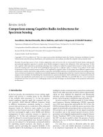
Example 2 (conventional LP of synthetic audio signal).
When we estimate a conventional LP model of order 2P
=
2N = 30 for the synthetic audio signal defined in Example 1,
using the covariance method [1] to calculate the model
parameters, we obtain a PEF as illustrated by the pole-
zero plot and magnitude response in Figures 2(a) and 2(b),
respectively. The conventional LP model nearly succeeds at
correctly modeling all the tonal components in the synthetic
audio signal. However, if we add Gaussian white noise to the
observed signal, the covariance method yields the estimated
conventional LP model shown in Figures 3(a) and 3(b),
for a signal-to-noise ratio (SNR) of 25 dB. The PEF zero
configuration is in this case clearly a compromise between
the LP solutions to the tonal part and the noise part of
the signal. The PEF has 9 complex conjugate zero pairs
in the sum of sinusoids frequency region, and another 6
complex conjugate zero pairs which are nearly uniformly
distributed in the upper half of the Nyquist interval. A
similar result is obtained when we use the autocorrelation
method [1] instead of the covariance method to predict the
noiseless synthetic audio signal. Indeed, the autocorrelation

method introduces noise in the autocorrelation domain by
distorting the signal periodicity due to zero padding. This
example illustrates the above statement that for conventional
LP models, the PEF zero configuration is a tradeoff between
suppressing the tonal components and keeping the noise
spectrum as flat as possible. Note that in the absence of noise
(Figure 2(b)), the PEF high-frequency response may become
extremely large.
4. ALTERNATIVE LINEAR PREDICTION MODELS
In this section, we present five existing alternative LP
models, and we illustrate how all these models attempt
to compensate for the shortcomings of the conventional
T. van Waterschoot and M. Moonen 7
−1
−0.8
−0.6
−0.4
−0.2
0
0.2
0.4
0.6
0.8
1
Imaginary part
−1 −0.50 0.51
Real part
30
(a)
−30

−25
−20
−15
−10
−5
0
5
10
15
20
20 log
10
|H(e
j2πf/f
s
)| (dB)
00.511.52
×10
4
f (Hz)
(b)
Figure 3: Conventional LP model of synthetic audio signal plus noise (SNR = 25 dB) with order 2P = 30 and covariance method: (a) PEF
pole-zero plot, (b) PEF magnitude response.
LP model, described in Section 3, when the input signal
tonal components are concentrated in the lower half of the
Nyquist interval. In the first three alternative LP models,
namely, the constrained pole-zero LP (PZLP) model, the
high-order LP (HOLP) model, and the pitch prediction
(PLP) model, the influence of the input signal frequency
distribution is decreased by using a model different from

the conventional low-order all-pole model. In the last two
alternative LP models, namely, the warped LP (WLP) model
and the selective LP (SLP) model, the performance of the
conventional low-order all-pole model is increased by first
transforming the input signal such that its tonal components
are spread in the entire Nyquist interval. As stated earlier, we
will mainly focus on the alternative LP models, and not on
how the model parameters can be estimated.
4.1. Constrained pole-zero LP model
It is well known that whereas a sum of N sinusoids can
be exactly modeled using an AR(2N)model,asumofN
sinusoids plus white noise should be modeled using an
ARMA(2N,2N)model[21–24]withequalcoefficients in the
AR and MA parts, that is, the zeros coinciding with the poles
[23, 25]. This observation can be extended to a sum of (finite-
bandwidth) damped sinusoids plus white noise, but in this
case the zeros should be slightly displaced toward the origin,
remaining on the same radial line as the poles [24, 25]. The
LP model in (7) can then be simplified to a constrained pole-
zero LP (PZLP) model with an equal number of poles and
zeros:
G(z)
=
P

l=1

1 −2ρ
l
cos θ

l
z
−1
+ ρ
2
l
z
−2


1 −2ν
l
cos θ
l
z
−1
+ ν
2
l
z
−2

(26)
with the constraint being that the poles and zeros are on the
same radial lines, that is, ζ
l
= θ
l
, l = 1, , P, with the poles
positioned between the zeros and the unit circle, that is, 0


ρ
l
< ν
l
≤ 1, l = 1, , P.
We now analyze the PZLP model performance for
predicting tonal signals corresponding to the signal model
(1), when P
= N, by substituting the PEF magnitude
response
|H(e
jω
)|
2
, obtained by inverting the magnitude
response of G(z)in(26), in the LP criterion (13). First, we
evaluate the second term of the LP criterion (13). Using the
direct-form representation of the PZLP model in (6), with
Q
= P and b
0
= 1, the PEF magnitude response can be
calculated as


H

e
jω




2
=


A

e
jω



2


B

e
jω



2
(27)
=
r
a
(0) + 2


2P
i=1
cos(iω)r
a
(i)
r
b
(0) + 2

2P
i=1
cos(iω)r
b
(i)
(28)
with r
a
(i) =

2P
p=i
a
p
a
p−i
and r
b
(i) =


2P
p=i
b
p
b
p−i
the
autocorrelation functions of the PEF numerator and denom-
inator coefficients, respectively. Note that when predicting
tonal signals, the PEF poles and zeros are typically very close
to the unit circle, and the PEF zeros are allowed to lie on
the unit circle. We can then approximately state that the
PEF pole radii are equal, that is, ρ
1
=···=ρ
P
= ρ and
likewise that the PEF zero radii are equal, that is, ν
1
=···=
ν
P
= ν. In this case, the numerator and denominator of the
PEF transfer function admit a particular structure, as shown
in [31]:
H(z) =
1+νg
1
z
−1

+ ···+ ν
P−1
g
P−1
z
−P+1
+ ν
P
g
P
z
−P
+ ν
P+1
g
P−1
z
−P−1
+ ···+ ν
2P−1
g
1
z
−2P+1
+ ν
2P
z
−2P
1+ρg
1

z
−1
+ ···+ ρ
P−1
g
P−1
z
−P+1
+ ρ
P
g
P
z
−P
+ ρ
P+1
g
P−1
z
−P−1
+ ···+ ρ
2P−1
g
1
z
−2P+1
+ ρ
2P
z
−2P

, (29)
8 EURASIP Journal on Audio, Speech, and Music Processing
and, as a consequence, the autocorrelation function of
the PEF numerator coefficients can be rewritten, for i
=
0, ,2P,as
r
a
(i) =
⎧
⎪
⎪
⎪
⎪
⎪
⎪
⎪
⎪
⎪
⎪
⎪
⎪
⎪
⎪
⎪
⎪
⎪
⎪
⎪
⎪

⎪
⎨
⎪
⎪
⎪
⎪
⎪
⎪
⎪
⎪
⎪
⎪
⎪
⎪
⎪
⎪
⎪
⎪
⎪
⎪
⎪
⎪
⎪
⎩
P−i

p=0
g
p
g

p+i

ν
2p+i
+ ν
4P−(2p+i)

+
(i−1)/2

p=1
g
P−p
g
P−i+p

ν
2P−i
+ ν
2P+i

, i = odd,
P−i

p=0
g
p
g
p+i


ν
2p+i
+ ν
4P−(2p+i)

+
(i/2)−1

p=1
g
P−p
g
P−i+p

ν
2P−i
+ ν
2P+i

+g
2
P
−(i/2)
ν
2P
, i = even,
(30)
and similarly for r
b
(i), i = 0, ,2P, by replacing ν with ρ in

(30). Since ν and ρ areassumedtobecloseto1,wecanmake
the following approximations:
ν
2p+i
+ ν
4P−(2p+i)
≈ 2ν
2P
, i = 0, ,2P, p = 0, , P −i,
ν
2P−i
+ ν
2P+i
≈ 2ν
2P
, i = 0, ,2P, p = 1, ,

i −1
2

,
ρ
2p+i
+ ρ
4P−(2p+i)
≈ 2ρ
2P
, i = 0, ,2P, p = 0, , P −i,
ρ
2P−i

+ ρ
2P+i
≈ 2ρ
2P
, i = 0, ,2P, p = 1, ,

i −1
2

,
(31)
where
x denotes the floor function, which returns the
highest integer less than or equal to x.Wecanhencerewrite
r
a
(i)in(30)andr
b
(i)as
r
a
(i) = ν
2P
γ
i
, i = 0, ,2P,
r
b
(i) = ρ
2P

γ
i
, i = 0, ,2P
(32)
with
γ
i
=
⎧
⎪
⎪
⎪
⎪
⎪
⎪
⎨
⎪
⎪
⎪
⎪
⎪
⎪
⎩
2
P−i

p=0
g
p
g

p+i
+2
(i−1)/2

p=1
g
P−p
g
P−i+p
, i = odd,
2
P−i

p=0
g
p
g
p+i
+2
(i/2)−1

p=1
g
P−p
g
P−i+p
+ g
2
P
−i/2

, i = even.
(33)
Substituting (32)in(28) yields


H

e
jω



2
=
ν
2P

γ
0
+2

2P
i
=1
cos(iω)γ
i

ρ
2P


γ
0
+2

2P
i=1
cos(iω)γ
i

=
ν
2P
ρ
2P
, (34)
which is expected to be a good approximation except in
the close neighborhood of the PEF pole-zero angles θ
l
, l =
1, , P, where the PEF magnitude response approaches zero
because the PEF zeros are closer to the unit circle than
the poles. However, when integrating the PEF magnitude
response over the entire frequency range [0, 2π), the notches
in
|H(e
jω
)|
2
at ω = θ
l

are negligible, such that the second
term in the LP criterion (13)canbewrittenas
σ
2
r
2π

2π
0


H

e
jω



2
dω = σ
2
r
ν
2P
ρ
2P
. (35)
We now consider the minimization of the LP criterion
(13) for the PZLP model (26), assuming that ν
1

=···=
ν
P
= ν and ρ
1
= ··· = ρ
P
= ρ with 0  ρ<ν ≤ 1and
using the approximation (31) such that the result in (35)can
be applied. Since ν and ρ are close to each other, they cannot
be treated as independent variables, and minimizing the LP
criterion with respect to ν and ρ can be achieved by setting
the total derivative with respect to ν and ρ to zero, which
leads to the following system of equations:
∂J(ξ)
∂θ
l
=
N

n=1
α
2
n
2

∂
∂θ
l



H

e
jω



2

ω=ω
n
+
∂
∂θ
l

σ
2
r
ν
2P
ρ
2P

=
0, l = 1, , P,
(36)
dJ(ξ)
dν

=
∂J(ξ)
∂ν
+
∂J(ξ)
∂ρ
dρ
dν
= 0,
(37)
dJ(ξ)
dρ
=
∂J(ξ)
∂ρ
+
∂J(ξ)
∂ν
dν
dρ
= 0
(38)
with
∂J(ξ)
∂ν
=
N

n=1
α

2
n
2

∂
∂ν


H

e
jω



2

ω=ω
n
+
∂
∂ν

σ
2
r
ν
2P
ρ
2P


=
0,
∂J(ξ)
∂ρ
=
N

n=1
α
2
n
2

∂
∂ρ


H

e
jω



2

ω=ω
n
+

∂
∂ρ

σ
2
r
ν
2P
ρ
2P

=
0.
(39)
Since ν and ρ are close to each other, we can assume
dρ
dν
≈
dν
dρ
≈ 1. (40)
Moreover,
∂
∂ν

σ
2
r
ν
2P

ρ
2P

≈−
∂
∂ρ

σ
2
r
ν
2P
ρ
2P

. (41)
Substituting (39)–(41)in(37)and(38) and noting that
the expression in (35) does not depend on the PEF pole-
zero angles θ
l
, we can see that all the terms in the system
of (36)–(38) that are due to the noise component in the
observed signal cancel out. In other words, if the PEF poles
and zeros are close to the unit circle, then the solution to the
LP estimation problem using the PZLP model is insensitive
to (white) noise in the observed signal. This is the main
strength of the PZLP model as compared to the conventional
LP model, which was shown in Section 3 to be much more
sensitive to noise when predicting tonal signals.
It remains to show that the PEF angles calculated

from (36)–(38) converge to the frequencies of the tonal
components. The PZLP PEF magnitude response and its
T. van Waterschoot and M. Moonen 9
partial derivatives with respect to θ
l
, l = 1, , P, ν,andρ
can be calculated as


H

e
jω



2
=
P

l=1


A
l

e
jω




2


B
l

e
jω



2
=
P

l=1

1−ν
2

2
+4ν
2

cos ω−cos θ
l

2
−4ν(1−ν)

2
cos θ
l
cos ω

1−ρ
2

2
+4ρ
2

cos ω−cos θ
l

2
−4ρ(1−ρ)
2
cos θ
l
cos ω
,
∂
∂θ
l


H

e

jω



2
=


B
l

e
jω



2
{C}


A
l

e
jω



2
−



A
l

e
jω



2
{C}


B
l

e
jω



2


B
l

e
jω




4
×
P

k=1
k
/
=l


A
k

e
jω



2


B
k

e
jω




2
,
∂
∂ν


H

e
jω



2
=
P

l=1

(∂/∂ν)


A
l

e
jω




2


B
l

e
jω



2
P

k=1
k
/
=l


A
k

e
jω




2


B
k

e
jω



2

,
∂
∂ρ


H

e
jω



2
=−
P

l=1




A
l

e
jω



2
(∂/∂ρ)


B
l

e
jω



2


B
l

e

jω



4
P

k=1
k
/
=l


A
k

e
jω



2


B
k

e
jω




2

,
(42)
where
{C} denotes (∂/∂θ
l
)with
∂
∂θ
l


A
l

e
jω



2
= 4ν sin θ
l

1+ν
2


cos ω − 2ν cos θ
l

,
∂
∂θ
l


B
l

e
jω



2
= 4ρ sin θ
l

1+ρ
2

cos ω − 2ρ cos θ
l

,
∂
∂ν



A
l

e
jω



2
= 4[2ν

cos ω − cos θ
l

2
−(1−ν)(1−3ν)cosθ
l
cos ω−ν

1−ν
2

,
∂
∂ρ


B

l

e
jω



2
= 4[2ρ

cos ω − cos θ
l

2
−(1−ρ)(1−3ρ)cosθ
l
cos ω−ρ

1−ρ
2

.
(43)
The global minimum of (13)withP = N, corresponding to
J(ξ)
= σ
2
r
, is obtained when



A
l

e
jω
l



2
= 0, l = 1, , P,
∂
∂θ
l


A
l

e
jω
l



2
= 0, l = 1, , P,
∂
∂ν



A
l

e
jω
l



2
= 0,
(44)
or, equivalently,
θ
l
= ω
l
, l = 1, , P,
ν
= 1,
(45)
and, hence, following the assumption that the PEF poles are
close to the zeros, ρ
→ 1.
Example 3 (constrained pole-zero LP of synthetic audio
signal). The PZLP model parameters can be estimated,
either using an adaptive notch filtering (ANF) algorithm, for
which several implementations have been suggested [24, 25,

31–35], or using the constrained pole-zero linear prediction
(CPZLP) algorithm for multitone frequency estimation [36,
37]. Alternatively, if the PEF pole and zero radii are fixed a
priori, any existing frequency estimation algorithm may be
used to estimate the unknown PEF angles. When harmonic-
ity can be assumed, that is, for monophonic audio signals,
an adaptive comb filter (ACF) may be a useful alternative to
the ANF, as it relies on only one unknown parameter (i.e.,
the fundamental frequency) [32, 35]. Similarly, a comb filter-
based variant of the CPZLP algorithm has been described in
[37].
Figures 4(a) and 4(b) show the PEF pole-zero plot and
magnitude response of a PZLP model of the synthetic audio
signal introduced in Example 1, and with additive Gaussian
white noise (SNR
= 25 dB). The PZLP model parameters
were calculated using the CPZLP algorithm with a comb
filter model [37]oforder2P
= 30, pole radius ρ = 0.95,
and zero radius ν
= 1, and with a numerical line search
method using the BFGS quasi-Newton algorithm with initial
fundamental frequency estimate ω
(0)
0
= 0.001 and line search
parameters as suggested in [36]. It can be seen that the
PEF magnitude response exhibits a notch filter behavior
at the frequencies of the tonal components, while being
approximately flat in the remainder of the Nyquist interval.

4.2. High-order LP model
It is well known that a pole-zero model can be arbitrarily
closely approximated with an all-pole model, provided that
the model order is chosen large enough. This means that a
noisy sum of sinusoids can also be modeled using a high-
order all-pole model instead of a pole-zero model [22]. In
Section 3, the LP minimization problem (13) was analyzed
for the case of an all-pole model of order P
= N. When
noise is present in the observed signal, the LP solution was
shown to be a compromise between cancelling the tonal
components and maintaining a flat high-frequency residual
spectrum. By increasing the model order, the density of the
zeros near the unit circle is increased accordingly, and hence
the frequency resolution in the tonal components frequency
range improves without sacrificing high-frequency residual
spectral flatness. However, as the LP model order 2P
approaches the observation window length L, the variance
of the estimated model parameters may be unacceptably
large, leading to spurious peaks in the signal spectral estimate
[22]. It has been suggested that the order 2P of a high-
order LP (HOLP) model should be chosen in the interval
10 EURASIP Journal on Audio, Speech, and Music Processing
−1
−0.8
−0.6
−0.4
−0.2
0
0.2

0.4
0.6
0.8
1
Imaginary part
−1 −0.50 0.51
Real part
(a)
−100
−80
−60
−40
−20
0
20
20 log
10
|H(e
j2πf/f
s
)| (dB)
00.511.52
×10
4
f (Hz)
(b)
Figure 4: Constrained pole-zero LP model of synthetic audio signal plus noise (SNR = 25 dB) with order 2P = 30 and CPZLP algorithm:
(a) PEF pole-zero plot, (b) PEF magnitude response.
2
2

2
2
2
2
2
2
1024
−1
−0.8
−0.6
−0.4
−0.2
0
0.2
0.4
0.6
0.8
1
Imaginary part
−1 −0.50 0.51
Real part
(a)
−50
−40
−30
−20
−10
0
10
20

20 log
10
|H(e
j2πf/f
s
)| (dB)
00.511.52
×10
4
f (Hz)
(b)
Figure 5: High-order LP model of synthetic audio signal plus noise (SNR = 25 dB) with order 2P = 1024 and autocorrelation method: (a)
PEF pole-zero plot, (b) PEF magnitude response.
L/3 ≤ 2P ≤ L/2 to obtain the best spectral estimate for a
noisy sum of sinusoids [22, 46].
Example 4 (high-order LP of synthetic audio signal). Per-
forming a L/2
= 1024th-order LP of the noisy synthetic
audio signal fragment defined before, using the autocorre-
lation method to estimate the model parameters, we obtain
a PEF pole-zero plot and magnitude response as shown in
Figures 5(a) and 5(b). Examining the distribution of the
PEF zeros in the complex plane reveals that this approach
produces approximately 1024
−2N zeros, lying on and nearly
equally spaced around the unit circle (to provide overall
spectral flatness of the PEF magnitude response), and 2N
additional zeros at the frequencies
±nω
0

, n = 1, , N of
the tonal components (to provide the notch filter behavior).
Note that when applying the covariance method to the
estimation of the HOLP model parameters, a similar result
is obtained.
4.3. Pitch prediction model
In LP of speech signals, the conventional LP model is usually
cascaded with the so-called pitch prediction (PLP) model,
with the aim of removing the long-term correlation from
the signal. This technique can also be used to remove the
(quasi) periodicity from monophonic audio signals, since it
implicitly relies on the harmonicity of the observed signal.
If we consider a sum of harmonic sinusoids having a pitch
period T
0
that corresponds to an integer number of sampling
periods KT
s
,whereK is referred to as the pitch lag, then
perfect prediction can be obtained by using a one-tap pitch
predictor, of which the PEF transfer function is given by
H(z)
= 1 −z
−K
= 1 −z
−T
0
/T
s
= 1 −z

−2π/ω
0
. (46)
The PEF magnitude response corresponding to (46)is


H

e
jω



2
= 2

1 −cos

2πω
ω
0

. (47)
T. van Waterschoot and M. Moonen 11
It can be seen that |H(e
jω
)|
2
= 0atω = kω
0

, ∀k ∈ Z,
which corresponds to a comb filter behavior, that is, the PEF
zeros are positioned on and equally spaced around the unit
circle, at angles corresponding to integer multiples of the
fundamental frequency ω
0
. In other words, referring to the
analysis in Section 3, the requirements of having the PEF
zeros on the unit circle at angles nω
0
, n = 1, , N (for
cancelling the tonal components) and uniformly distributed
on the unit circle (for maintaining the LP residual spectral
flatness) are both fulfilled with the PLP model in (46).
However, for the PLP model to be capable of producing
a good spectral estimate of a monophonic audio signal,
we should improve the model in (46)intwoways.First
of all, in audio signals the amplitudes of the harmonics
nω
0
typically decrease with increasing n (see, e.g., Figures
11(b) and 14(b) in Section 5). This effect requires the PEF
magnitude response to be spectrally shaped such that the
comb filter notch depth decreases for increasing frequency.
This can be achieved by using a multitap PLP model [47]
which features multiple nonzero filter coefficients centered
around the pitch lag value. In speech processing, a 3-tap
PLP model is often applied, since this configuration usually
provides enough flexibility in terms of spectral shaping:
H(z)

= 1+a
K−1
z
−(K−1)
+ a
K
z
−K
+ a
K+1
z
−(K+1)
. (48)
From the 3-tap PEF magnitude response


H

e
jω



2
=

cos Kω + a
K
+


a
K−1
+ a
K+1

cos ω

2
+

sin Kω+

a
K−1
−a
K+1

sin ω

2
,
(49)
it can be derived that the desired spectral shaping for our
application, that is, a decreasing notch depth for increasing
frequency, is obtained when
−1 ≤ a
K
< (a
K−1
+ a

K+1
) < 0
[47].
Secondly, the PLP model in (47) is based on the
assumption that the pitch lag K
= T
0
/T
s
is an integer
number, which is generally not the case. Noninteger pitch
lags can be incorporated in the PLP model in two ways:
either by using a multitap PLP model for interpolation (see,
e.g., [2]) or by using a fractional delay filter [48], for which
numerous design methods exist [49]. We prefer to combine
both approaches, such that the multitap structure may be
primarily used for spectral shaping, whereas interpolation
for noninteger pitch lags is achieved with a fractional delay
filter. A combined fractional multitap PLP model has been
proposed in [47], with
H(z)
= 1+
K+1

l=K−1
a
l
z
−l
×


I−1

i=−I
w
h

I +
f
D

sinc

I +
f
D

z
i

.
(50)
The fractional delay interpolation filter is a Hamming-
windowed, truncated (length-2I) approximation of the ideal
sinc-like interpolation filter [49], with w
h
(t) denoting the
Hamming window (centered at t
= 0). In (50), D is the
interpolation ratio (where 1/D is referred to as the pitch

resolution) and f
= 0,1, , D − 1 denotes the fractional
phase.
Typically, for estimating the PLP model parameters, in
a first step, the optimal pitch lag K and fractional phase
f are estimated by an exhaustive search of the minimal
fractional 1-tap PLP residual power over the interval K
∈
[K
min
, K
max
]and f ∈ [0, D − 1]. In speech analysis, the
pitch lag limits correspond to the highest-pitched (female)
and lowest-pitched (male) voices being analyzed and are
typically chosen in the range K
min
= 20, ,40and K
max
=
120, , 160 samples, at f
s
= 8kHz. For pitch analysis of
audio signals, we propose to set the pitch lag range such
that it corresponds to a fundamental frequency range of
100, , 1000 Hz, that is, at f
s
= 44.1 kHz, K ∈ [44, 441].
In a second step, the fractional 3-tap PLP model parameters
a

l
, l ∈ [K − 1, K + 1] are estimated using the estimated
pitch lag and fractional phase from the first step. Some
useful approximations for efficiently calculating the 3-tap
PLP model parameters from the input signal autocorrelation
function have been suggested in [2].
Example 5 (pitch prediction of synthetic audio signal). The
parameters of the fractional 3-tap PLP model given in
(50) were estimated for the noisy synthetic audio signal
defined earlier using the method proposed in [47], with an
interpolation filter of length 2I
= 32 and an interpolation
ratio D
= 8, and by forcing the input correlation matrix
to be Toeplitz [2]. The resulting PEF magnitude response
and pole-zero plot are shown in Figures 6(a) and 6(b).
Note the additional circle of zeros around the origin in
Figure 6(a), which is due to the fractional part of the
PEF transfer function, and the spectral shaping effect in
Figure 6(b), which is obtained by using multiple taps in the
PLP model.
4.4. Warped LP Model
Warped linear prediction (WLP) is probably the most well-
known technique for LP of audio signals, see [12]and
references therein. In WLP, the input signal undergoes a
nonuniform frequency transformation before a conventional
LP is performed, with the aim of enhancing the frequency
resolution in certain frequency regions. The frequency
transformation is usually defined by an all-pass bilinear
transform in the z-domain, which maps the unit circle onto

itself:
z
−1
−→ z
−1
=
z
−1
−λ
1 −λz
−1
. (51)
The so-called warping parameter λ is typically chosen such
that the corresponding frequency mapping
ω
−→ ω = ω + 2 arctan

λ sin ω
1 −λ cos ω

(52)
12 EURASIP Journal on Audio, Speech, and Music Processing
81
−1
−0.8
−0.6
−0.4
−0.2
0
0.2

0.4
0.6
0.8
1
Imaginary part
−1 −0.50 0.51
Real part
(a)
−40
−35
−30
−25
−20
−15
−10
−5
0
5
10
20 log
10
|H(e
j2πf/f
s
)| (dB)
00.511.52
×10
4
f (Hz)
(b)

Figure 6: Fractional 3-tap PLP model of synthetic audio signal plus noise (SNR = 25 dB): (a) PEF pole-zero plot, (b) PEF magnitude
response.
approximates the Bark auditory scale [30], that is, when the
sampling rate f
s
is expressed in kHz:
λ
Bark

f
s

=
1.0674

2
π
arctan

0.06583 f
s

−0.1916.
(53)
Since λ
Bark
(44.1) > 0, the warping operation tends to
spread out the tonal components in the observed signal
over the entire Nyquist interval. From the conventional
LP analysis in Section 3, it can hence be expected that

applying a conventional, that is, low-order all-pole LP model
to the warped signal will yield a better prediction than a
conventional LP model of the original signal. The optimal
prediction is obtained when the frequency transformation
produces a uniform spreading of the tonal components in
the Nyquist interval. For monophonic audio signals, this
is never the case, since the bilinear frequency warping in
(51)-(52) disturbs the harmonicity of the signal. For this
class of signals, the frequency transformation of the selective
LP model described in Section 4.5 appears to be better
suited. However, for polyphonic audio signals, the above
bilinear frequency warping may be a near-optimal mapping,
since in this case the different fundamental frequencies are
approximately related to each other according to the Bark
scale (see also the simulation results in Section 5.3).
Example 6 (warped LP of synthetic audio signal). The
warped spectrum of the noisy synthetic audio signal defined
before is shown in Figure 7(a) for λ
= λ
Bark
(44.1) =
0.75641. Figures 7(b) and 7(c) illustrate the PEF pole-zero
plot and magnitude response on a warped frequency scale

f = ω( f
s
/2π), when a 2Nth-order WLP model is calculated
using the autocorrelation method. The frequency resolution
of the signal WLP spectral estimate is very good for the five
lowest tonal components nω

0
, n = 1, , 5, while the higher
harmonics are modeled less accurately because they are
too closely spaced on the warped frequency scale. The PEF
transfer function can be unwarped to the original frequency
scale, but then the PEF impulse response is of infinite
duration. The PEF pole-zero plot and magnitude response
on the original frequency scale, obtained by truncating the
unwarped PEF impulse response to a length of L/4
= 512
samples, are shown in Figures 7(d) and 7(e). The pole-zero
plot on the original frequency scale clearly illustrates that the
WLP model succeeds both at cancelling the (low-frequency)
tonal components (by placing a few zeros approximately on
the unit circle at the lower tonal component frequencies) and
at preserving the overall spectral flatness of the residual (by
placing a large number of zeros uniformly spaced around and
close to the unit circle).
Note that the WLP residual e(t,ξ) can be calculated
without unwarping the PEF transfer function, but instead by
considering the PEF as a warped FIR filter [50]. Moreover,
before feeding the WLP residual to a synthesis filter or
calculating its spectral flatness (see Section 5), it should be
postfiltered with a high-pass filter defined as [12]
D
−1
0
(z) =
1 −λz
−1

√
1 −λ
2
. (54)
4.5. Selective LP Model
In some cases, for example, when dealing with monophonic
audio signals, a uniform frequency mapping may be more
useful than a nonuniform mapping such as the warping
operation described in Section 4.4, since it preserves the
harmonic relation between the tonal components. A uniform
mapping, which allows to “zoom in” on a certain frequency
region ω
1
≤ ω ≤ ω
2
, is accomplished by
ω
−→ ω = π
ω
−ω
1
ω
2
−ω
1
(55)
which, when combined with a conventional LP model, is
known as a selective LP (SLP) model [1].
To obtain a uniform spreading of the tonal components
over the entire Nyquist interval, we should choose ω

1
= 0
T. van Waterschoot and M. Moonen 13
−20
−10
0
10
20
30
40
50
60
20 log
10
|X(e
j2π

f/f
s
)| (dB)
00.511.52
×10
4

f (Hz)
(a)
30
−1
−0.8
−0.6

−0.4
−0.2
0
0.2
0.4
0.6
0.8
1
Imaginary part
−1 −0.50 0.51
Real part
(b)
−40
−30
−20
−10
0
10
20
20 log
10
|H(e
j2π

f/f
s
)| (dB)
00.511.52
×10
4


f (Hz)
(c)
512
−1
−0.8
−0.6
−0.4
−0.2
0
0.2
0.4
0.6
0.8
1
Imaginary part
−1 −0.50 0.51
Real part
(d)
−40
−30
−20
−10
0
10
20
20 log
10
|H(e
j2πf/f

s
)| (dB)
00.511.52
×10
4
f (Hz)
(e)
Figure 7: Warped LP model of synthetic audio signal plus noise (SNR = 25 dB) with order 2P = 30, warping parameter λ = λ
Bark
(44.1),
and autocorrelation method: (a) Noisy synthetic audio signal magnitude spectrum (warped scale), (b) PEF pole-zero plot (warped scale),
(c) PEF magnitude response (warped scale), (d) PEF pole-zero plot (original scale), (e) PEF magnitude response (original scale).
and ω
2
= ω
1
+ ω
N
,withω
1
and ω
N
the frequencies of the
lowest and highest tonal components, see (1). This leads to
ω
−→ ω = Γω (56)
with
Γ
=
π

ω
1
+ ω
N
. (57)
In the z-domain, this corresponds to the mapping:
z
−1
−→ z
−1
= z
−Γ
, (58)
which is a downsampling operation with downsampling
factor Γ. In the case of a monophonic audio signal, the
downsampling factor can be rewritten using (2):
Γ
=
π
(N +1)ω
0
=
f
s
2(N +1)f
0
, (59)
and in the polyphonic case, using (3):
Γ =
π

ω
0,1
+ M
N
ω
0,N
=
f
s
2

f
0,1
+ M
N
f
0,N

. (60)
Note that the optimal downsampling factor Γ,givenin
(57), is highly signal-dependent, and noninteger downsam-
pling is required in general. These difficulties can be easily
avoided by using an approximate, integer downsampling
factor (see Section 5) which is chosen to be fixed for the
entire signal analysis. It should then typically be chosen in the
range Γ
= 2, , 10, if possible, using some prior knowledge
about the frequency range of the instrument generating the
audio signal being analyzed.
Example 7 (selective LP of synthetic audio signal). The

spectrum of the noisy synthetic audio signal defined before,
downsampled with a factor Γ
= 2 (obtained from (59)with
ω
0
= 2π/64 and N = 15), is shown in Figure 8(a),and
the PEF pole-zero plot and magnitude response, resulting
from using a 2Nth-order SLP model, calculated with the
autocorrelation method, are plotted on the downsampled
frequency scale in Figures 8(b) and 8(c). The PEF zeros are
nearly perfectly distributed in a uniform way around the
unit circle with exactly one complex conjugate zero pair
for each tonal component in the downsampled signal. After
upsampling, the PEF pole-zero plot and magnitude response
shown in Figures 8(d) and 8(e) are obtained. The PEF
behavior on the original frequency scale is comparable to the
PLP model PEF behavior, that is, nearly perfect cancellation
of the tonal components is achieved, at the cost of having
additional notches in the upper half of the Nyquist interval,
which may result in a nonsmooth high-frequency residual
spectrum. The LP residual can either be calculated on the
downsampled or on the original time scale.
14 EURASIP Journal on Audio, Speech, and Music Processing
−20
−10
0
10
20
30
40

50
60
20 log
10
|X(e
j2πK f/f
s
)| (dB)
0 2000 4000 6000 8000 10000
f (Hz)
(a)
30
−1
−0.8
−0.6
−0.4
−0.2
0
0.2
0.4
0.6
0.8
1
Imaginary part
−1 −0.50 0.51
Real part
(b)
−30
−20
−10

0
10
20
30
20 log
10
|H(e
j2πK f/f
s
)| (dB)
0 2000 4000 6000 8000 10000
f (Hz)
(c)
60
−1
−0.8
−0.6
−0.4
−0.2
0
0.2
0.4
0.6
0.8
1
Imaginary part
−1 −0.50 0.51
Real part
(d)
−30

−20
−10
0
10
20
30
20 log
10
|H(e
j2πf/f
s
)| (dB)
00.511.52
×10
4
f (Hz)
(e)
Figure 8: Selective LP model of synthetic audio signal plus noise (SNR = 25 dB) with order 2P = 30, downsampling factor Γ = 2, and
autocorrelation method: (a) noisy synthetic audio signal magnitude spectrum (downsampled scale), (b) PEF pole-zero plot (downsampled
scale), (c) PEF magnitude response (downsampled scale), (d) PEF pole-zero plot (original scale), (e) PEF magnitude response (original
scale).
5. SIMULATION RESULTS
In this section, we evaluate the conventional and alternative
LP models described in Sections 3 and 4 in terms of
frequency estimation accuracy, residual spectral flatness, and
perceptual frequency resolution for a synthetic harmonic
audio signal with varying fundamental frequency and SNR.
Afterwards, we apply the different LP models to true
monophonic and polyphonic audio signals, and we analyze
the PEF behavior by examining the pole-zero plots and

magnitude responses. Residual spectral flatness figures are
given for true audio signals as a function of pitch and time
offset of the analysis window within the signal.
We should stress that the aim is to compare different
LP models, and not the algorithms that can be used to
estimate the model parameters. Some models come with
parameter estimation algorithms that are well established
(e.g., covariance method or autocorrelation method with
Levinson-Durbin algorithm [51, Chapter 6] for all-pole
models), yet other models do not. In particular, PZLP
models typically result in a nonconvex parameter estimation
problem that is solved either in an adaptive or iterative way.
As a consequence, the performance of the corresponding
estimation algorithms (e.g., ANF or CPZLP) depends heavily
on the initial conditions. In the simulation results presented
below, the initial conditions are chosen in the neighborhood
of the true fundamental frequencies in the observed audio
signal, such that the PZLP estimation algorithms yield a
solution that corresponds with high probability to the global
solution. In this way, the emphasis is on the model perfor-
mance rather than on the estimation algorithm performance.
For the same reason, knowledge of the true fundamental
frequencies is also assumed when determining the optimal
downsampling factor in the SLP estimation algorithms, and
for designing a PLP model for polyphonic audio signals.
For the conventional LP model, the performance may
differ substantially for the autocorrelation and covariance
estimation methods, hence the results for both methods are
included.
5.1. Synthetic audio signal

Throughout Examples 2–7, the performance of conventional
and alternative LP models was illustrated by inspecting
the PEF pole-zero plots and magnitude responses, resulting
from the prediction of a noisy synthetic audio signal with
fundamental frequency f
0
≈ 689.1Hz and SNR = 25 dB.
We also present a more quantitative evaluation of the
different LP models, for a synthetic audio signal with variable
fundamental frequency and SNR.
T. van Waterschoot and M. Moonen 15
A first performance measure is the mean square fre-
quency error (MSFE), which is defined with the aim of
evaluating the frequency estimation accuracy of the different
LP models,
MSFE
=
1
N
N

n=1

θ
l(n)
−ω
n

2
(61)

with
l(n)
= arg min
l


ν
l
e
jθ
l
−e
jω
n


2
= arg min
l

1+ν
2
l
−2ν
l
cos

θ
l
−ω

n

.
(62)
In other words, the MSFE is calculated as the mean square
difference between each of the frequencies ω
n
of the N tonal
components in the observed signal, and the angle of the
PEF zero ν
l(n)
e
jθ
l(n)
that is closest to the point e
jω
n
in the
complex plane. The MSFE was calculated for a synthetic
audio signal with N, L, f
s
, α
n
,andφ
n
as in Example 2,
with additive Gaussian white noise resulting in an SNR
=
25 dB and with varying fundamental frequency equals to the
first 11 center frequencies of the Bark scale [52]. A second

experiment was conducted with similar signals having a fixed
fundamental frequency f
0
≈ 689.1 Hz, and an SNR varying
between
−50 dB and 50 dB in steps of 10 dB. The MSFE
results, averaged over 100 Monte Carlo trials for different
realizations of the Gaussian white noise sequence, are shown
in Figures 9(a) and 9(b). The MSFE of the low-order all-
pole models (LP
AUTO
,LP
COV
, WLP, and SLP) appears to be
more or less invariant with respect to varying fundamental
frequency and SNR, with MSFE values varying between
−50 and −20 dB, the highest of which is obtained with
the conventional LP model. It can be observed that models
for which the PEF zeros are on (PLP and PZLP) or very
close to (HOLP) the unit circle generally provide a higher
frequency estimation accuracy. The HOLP model produces
MSFE values between
−70 and −50 dB, which are invariant
with varying fundamental frequency, and slightly lower for
high than for low SNRs. At sufficiently high fundamental
frequency and SNR values, the PLP and PZLP models achieve
an MSFE as low as
−90 (PLP) and −100 (PZLP) dB.
However, the PLP and PZLP models MSFE performance is
seen to be worse for lower fundamental frequencies and SNR

values. The sensitivity of these models to the fundamental
frequency is presumably related to the fact that these are
the only models that explicitly rely on the harmonicity of
the observed signal (since in the PZLP case, the comb filter
model is used). The performance drop of the PZLP model
at low SNR values is due to the accuracy of the CPZLP
algorithm, which is known to be relatively poor at SNR values
below
−5dB[37].
A second performance measure is the spectral flatness
measure (SFM) of the LP residual, defined as [43,Chapter
6]
SFM
E
=
exp

(1/L)

L−1
k
=0
ln


E

e
j(2πk/L)
, ξ





(1/L)

L−1
k=0


E

e
j(2πk/L)
, ξ



(63)
with E(e
j(2πk/L)
, ξ), k = 0, ,L − 1 the L-point DFT of
the LP residual e(t, ξ).TheSFMisarealnumberbetween
0 and 1, with SFM
= 1 corresponding to a flat spectrum,
and is often expressed on a dB-scale (0 dB corresponding
to a flat spectrum). Monte Carlo simulation results of the
residual SFM after prediction of the synthetic audio signals
with varying fundamental frequency and SNR described
above are shown in Figures 9(c) and 9(d). The residual

SFM of the low-order all-pole models (LP
AUTO
,LP
COV
,WLP,
and SLP) decreases with increasing fundamental frequency
and increasing SNR. The first observation can be explained
by noting that at low fundamental frequency values, the
low-order all-pole models tend to model multiple tonal
components with one complex conjugate pole pair, while the
remaining poles are used to model the high-frequency noise
spectrum. As a consequence, most of the poles are located
relatively far away from the unit circle, hence resulting in
a smoother spectral behavior. The residual SFM drop at
high SNR values should not be surprising, since the low-
order all-zero PEFs generally do not succeed at completely
cancelling the tonal components from the observed signal.
On the other hand, the residual SFM of the PLP and PZLP
models can be seen to increase with increasing fundamental
frequency and decreases (PLP) or remains quasiconstant
(PZLP) with increasing SNR. The HOLP model residual
SFM is the highest among all LP models, and appears to
be independent of both fundamental frequency and SNR.
The SFM of the synthetic audio signals before LP was on
average
−10 dB in the varying fundamental frequency case,
and
−35 dB in the varying SNR case. A relevant extension to
the low-order alternative LP models described in Section 4
is to cascade them with a conventional LP model. Such a

cascaded model can be motivated by noting that for true
audio signals, the noise term in the tonal signal models
(1)–(3) may be nonwhite. Hence, an alternative LP model
could be applied first for predicting the tonal components,
and in a second step a conventional LP model could be
used for whitening both the noise and the unpredicted tonal
components in the residual of the alternative LP model. This
cascaded structure appears to be beneficial for the low-order
alternative LP models (PZLP, PLP, WLP, and SLP) in terms
of increasing the residual SFM, especially at high SNR values
and, for the PZLP and PLP models, also at low fundamental
frequency values.
Finally, the third performance measure we will use is the
interpeak dip depth (IDD) [12], a perceptually motivated
measure which reflects the separability of spectral peaks for a
certain model. It is defined for an LP model of a length-L sum
of two sinusoids at frequencies f
1
and f
2
Hz, separated by
two times the equivalent rectangular bandwidth (ERB) [53]
at the lower frequency f
1
, that is, f
2
= f
1
+2(0.108 f
1

+24.7),
as
IDD
=
L
1
+ L
2
2L
d
(64)
with L
1
and L
2
corresponding to the amplitude of the two
peaks in the LP model magnitude response, and L
d
to the
minimal amplitude between the two peaks. The higher the
IDD, the better the perceptual frequency resolution of the
16 EURASIP Journal on Audio, Speech, and Music Processing
−100
−90
−80
−70
−60
−50
−40
−30

−20
−10
0
MSFE (dB)
10
2
10
3
f
0
(Hz)
LP
COV
LP
AUTO
PZLP
HOLP
PLP
WLP
SLP
(a) MSFE (dB) versus fundamental frequency f
0
(Hz)
−120
−100
−80
−60
−40
−20
0

20
MSFE (dB)
−50 −40 −30 −20 −10 0 10 20 30 40 50
SNR (dB)
LP
COV
LP
AUTO
PZLP
HOLP
PLP
WLP
SLP
(b) MSFE (dB) versus SNR (dB)
−9
−8
−7
−6
−5
−4
−3
−2
−1
0
SFM
E
(dB)
10
2
10

3
f
0
(Hz)
LP
COV
LP
AUTO
PZLP
PZLP + LP
AUTO
HOLP
PLP
PLP + LP
AUTO
WLP
WLP + LP
AUTO
SLP
SLP + LP
AUTO
(c) Residual SFM (dB) versus fundamental frequency f
0
(Hz)
−14
−12
−10
−8
−6
−4

−2
0
SFM
E
(dB)
−50 −40 −30 −20 −10 0 10 20 30 40 50
SNR (dB)
LP
COV
LP
AUTO
PZLP
PZLP + LP
AUTO
HOLP
PLP
PLP + LP
AUTO
WLP
WLP + LP
AUTO
SLP
SLP + LP
AUTO
(d) Residual SFM (dB) versus SNR (dB)
Figure 9: Mean square frequency error (MSFE) and residual SFM curves of Monte Carlo simulations for a synthetic audio signal with
variable fundamental frequency and SNR.
model is expected to be. The IDD was measured for all LP
models except the PLP model, for 24 sets of two sinusoids,
with f

1
corresponding to the center frequency of the 24
Bark scale bands [52]. The PLP model is not appropriate
for this type of signal, since the sinusoid frequencies are not
harmonically related. The IDD results for the conventional
LP, PZLP, WLP, and SLP models with order 2P
= 2N = 4and
for the HOLP model with order 2P
= L/2 = 1024 are shown
in Figure 10. The low-order all-pole models perform poorly,
except for the conventional LP model with the covariance
T. van Waterschoot and M. Moonen 17
0
10
20
30
40
50
60
70
80
90
IDD (dB)
10
2
10
3
10
4
f

1
(Hz)
LP
COV
LP
AUTO
PZLP (ρ = 0.95)
PZLP (ρ
= 0.99)
HOLP
WLP
SLP
Figure 10: IDD results for two-tone signal with frequencies f
1
and
f
2
= f
1
+2ERB(f
1
).
estimation method, which has a very high IDD even in the
low-frequency region. For true audio signals, however, the
LP
COV
modelwillperformworseintermsofperceptual
frequency resolution since the estimated model parameters
can strongly differ for noise-free and noisy sinusoidal signals,
see Figures 2(a) and 3(a). The HOLP model IDD exhibits a

similar trend as the LP
COV
model IDD, as it slightly increases
with increasing frequency, remaining on average 14 dB below
the LP
COV
modelIDDcurve.ThePZLPmodelcanbeseen
to produce high IDD values at low and high frequencies,
but performs poorly in the midfrequency range (250 to
1370 Hz), which is exactly the frequency range of interest in
audio applications. Of course, the IDD performance of an
LP model is strongly related to the bandwidth of the spectral
peaks that it can produce. As a consequence, the PZLP model
IDD performance can be improved by increasing the pole
radius (e.g., ρ
= 0.99, see Figure 10), which is equivalent to
reducing the smallest achievable bandwidth [54], however,
when dealing with true audio signals a lower value of the
pole radius is expected to be more appropriate for taking into
account the damping of the tonal components.
5.2. Monophonic audio signal
A length-L monophonic audio fragment was extracted from
a Bb clarinet sound recording in the McGill University
Master Samples collection [55]. The fragment, which cor-
responds to the samples 70001 to 72048 of the G4 note
recording, is shown in Figure 11(a), along with its magni-
tude spectrum in Figure 11(b). The fundamental frequency
corresponds to f
0
= 387.6 Hz, and the number of relevant

harmonics is chosen to be N
= 15. A conventional LP
model of order 2P
= 30, calculated using the autocorrelation
method, produces a PEF as illustrated in Figures 12(a) and
12(d), which is again a compromise between cancelling
the tonal components and keeping the residual spectrum
relatively flat. A better resolution is obtained using a PZLP
model with 2P
= 30, ρ
l
= 0.95, and ν
l
= 1, l = 1, , P,as
shown in Figures 12(b) and 12(e), and using an HOLP model
with 2P
= 1024, see Figures 12(c) and 12(f).Afractional3-
tap PLP model was calculated using the method proposed
in [47], with the algorithm parameters given in Example 5,
resulting in the PEF shown in Figures 12(g) and 12(j),in
which the spectral shaping capability of the 3-tap PLP model
is clearly exploited. A WLP model with 2P
= 30 and λ =
λ
Bark
(44.1) produces an unwarped PEF as shown in Figures
12(h) and 12(k). Finally, the SLP model with 2P
= 30,
for which the optimal downsampling factor from (57)was
rounded to Γ

= 4, has a PEF after upsampling which is given
in Figures 12(i) and 12(l).
The residual SFM values obtained with the different LP
models were calculated for 2048 sample fragments taken
from the sustain part of the Bb clarinet recordings in [55]
with varying pitch, ranging from D3 to D6 (corresponding to
f
0
= 146.8 Hz to 1174.7 Hz), and are shown in Figure 13(a).
The original signal fragments have an average SFM value
of
−31 dB. The residual SFM curves for the PZLP and
PLP models are not shown, as they are (partially) outside
the displayed SFM range, with an average residual SFM
of
−12 and −19 dB, respectively. Figure 13(c) contains the
residual SFM results when the analysis window time offset
is varied in steps of 2048 samples from the onset till
the end of the Bb clarinet G4 note in [55], which is
plotted in Figure 13(b). Again, the PZLP and PLP curves
are omitted, with an average residual SFM of
−10 and
−19 dB, respectively, while the original signal fragments
have an average SFM of
−29 dB. From Figure 13(a),wecan
observe that the residual SFM does not exhibit a notable
trend with varying fundamental frequency for any of the LP
models, which is somewhat contradictory with the results
obtained for synthetic signals (see Figure 9(c)). This can
be explained by suggesting that the residual SFM value for

true audio signals is primarily determined by the (low-
power) harmonics which are modeled as noise components
instead of tonal components. This undermodelling effect is
generally independent of the fundamental frequency, but
rather depends on which musical instrument is considered.
Figures 13(b) and 13(c) show that the LP model performance
is comparable in the decay, sustain, and release part of
the note, but somewhat worse in the attack part. This is
mainly due to the fact that the attack part exhibits much less
stationarity than the other signal parts. In both experiments,
the HOLP model and the PZLP and PLP models cascaded
with a conventional LP model, provide the best residual
SFM results, which is consistent with the results obtained
for synthetic signals (see Figures 9(c) and 9(d)). The WLP
model, potentially cascaded with a conventional LP model,
performs somewhat worse yet still outperforms the LP
AUTO
model, while the SLP and LP
COV
models yield significantly
poorer results.
5.3. Polyphonic audio signal
From the concert hall Steinway recordings in [55], a
polyphonic audio signal was generated by adding four
monophonic piano sounds. The samples 2001 to 4048 of
18 EURASIP Journal on Audio, Speech, and Music Processing
−0.25
−0.2
−0.15
−0.1

−0.05
0
0.05
0.1
0.15
0.2
0.25
x(t)
00.01 0.02 0.03 0.04
t (s)
(a)
−40
−30
−20
−10
0
10
20
30
40
20 log
10
|X(e
j2πf/f
s
)| (dB)
00.511.52
×10
4
f (Hz)

(b)
Figure 11: Monophonic audio signal: (a) time-domain waveform, (b) magnitude spectrum.
the C4, E4, G4, and C5 note recordings were added to
obtain a length-L C major chord, plotted in Figures 14(a)
and 14(b). The four fundamental frequencies are f
0,n
=
{
258.4, 323, 387.6, 516.8}Hz, and each of the monophonic
components has 7 relevant harmonics, that is, M
n
= 7, n =
1, , 4. The PEF obtained with a conventional LP model of
order 2P
= 2

4
n
=1
M
n
= 54 is shown in Figures 15(a) and
15(d). It can be seen that the PEF has only one low-frequency
notch and an overall high-pass shape. The PZLP model with
2P
= 54, ρ
l
= 0.95, and ν
l
= 1, l = 1, ,P produces

exactly as many PEF notches as there are nonoverlapping
tonal components, as can be seen in Figures 15(b) and 15(e).
The same holds true for the HOLP model with 2P
= 1024,
of which the PEF is shown in Figures 15(c) and 15(f).
The PLP model does not seem to be suited for predicting
polyphonic signals since the tonal components do not obey
an integer harmonic relation. An alternative PLP approach
could exist in cascading as many PLP models as there are
different fundamental frequencies in the polyphonic signal,
but this does not yield good results. Another alternative
PLP approach may be based on the fractional harmonic
relations which exist between the fundamental frequencies in
a musical chord, for example, for a major chord (consisting
of dominant, third, fifth, and octave) it can be verified
that f
0,2
= (5/4) f
0,1
, f
0,3
= (3/2) f
0,1
,and f
0,4
= 2 f
0,1
.
As a consequence, a fractional PLP model with pitch lag
K

= 4(T
0,1
/T
s
) samples would produce PEF notches at all
the tonal components in the polyphonic signal. However,
allowing such large pitch lags deteriorates the performance
of the algorithm for calculating the PLP model parameters,
since the allowable pitch lag search space [K
min
, K
max
]
becomes very large, rendering the algorithm slower and less
reliable. Moreover, the large number of spurious notches in
the PEF frequency response leads to an extremely nonsmooth
residual spectrum. As an example, a fractional pseudo-3-
tap PLP model [47], assuming knowledge of the pitch lag
K
= 4(T
0,1
/T
s
) = 682.6625 samples, was constructed by
setting a
K−1
= a
K+1
=−0.05 and a
K

=−0.9. The resulting
PEF when 2I
= 32 and D = 8 is shown in Figures 15(g) and
15(j). Finally, the WLP and SLP models were applied to the
polyphonic signal, both with 2P
= 54, a warping parameter
λ
= λ
Bark
(44.1) resulting in the unwarped PEF in Figures
15(h) and 15(k), and a downsampling factor Γ
= 6(rounded
from the optimal value in (60)) resulting in the upsampled
PEF shown in Figures 15(i) and 15(l).
Two similar experiments as in the monophonic case
were performed, for calculating the residual SFM values
after prediction of a polyphonic audio signal with varying
pitch and analysis window time offset. Figure 16(a) shows
the residual SFM results for LP of a 4-note major chord
(consisting of dominant, third, fifth, and octave) created
from the concert hall Steinway recordings in [55], in which
the dominant varies from A0 to C7 (corresponding to
f
0
= 27.5 Hz to 2093 Hz), and the analysis window is in
the release part of the chord. The LP
COV
and PLP curves
are not shown, since they are partially below the displayed
residual SFM range, having a residual SFM value of

−11 and
−30 dB, respectively. The original polyphonic signals have
an average SFM of
−32 dB. At very low-pitched chords, the
LP
AUTO
, HOLP, WLP, SLP models and the PZLP and PLP
models cascaded with a conventional LP model are quite
competitive, however, toward higher pitch values, the HOLP
and WLP models outperform the other models. The superior
performance of the WLP model as compared to the other
low-order models should not be a surprise. As noted in
Section 4.4, the tonal components in a polyphonic signal are
approximately distributed according to the Bark scale and are
hence mapped to a nearly uniform frequency distribution
after frequency warping. The LP
AUTO
and SLP models still
perform reasonably well for high-pitched chords, while the
cascaded PZLP and PLP models perform worse. It appears
that the approach of decomposing the polyphonic signal into
a number of harmonic signals (which is what the PZLP and
PLP models attempt to do) is not beneficial in terms of resid-
ual spectral flatness. In Figure 16(b), the 4-note major chord
with dominant C4 is plotted, for which the residual SFM
results of LP with a variable analysis window time offset are
shown in Figure 16(c). During the attack part of the chord
(analysis window offset
= 0 second), all LP models perform
poorly. In the next 5 positions of the analysis window, which

T. van Waterschoot and M. Moonen 19
30
−1
−0.8
−0.6
−0.4
−0.2
0
0.2
0.4
0.6
0.8
1
Imaginary part
−1 −0.50 0.51
Real part
(a) Conventional LP model
−1
−0.8
−0.6
−0.4
−0.2
0
0.2
0.4
0.6
0.8
1
Imaginary part
−1 −0.50 0.51

Real part
(b) Pole-zero LP model
2
2
1024
−1
−0.8
−0.6
−0.4
−0.2
0
0.2
0.4
0.6
0.8
1
Imaginary part
−1 −0.50 0.51
Real part
(c) High-order LP model
−50
−40
−30
−20
−10
0
10
20
20 log
10

|H(e
j2πf/f
s
)| (dB)
00.511.52
×10
4
f (Hz)
(d) Conventional LP model
−120
−100
−80
−60
−40
−20
0
20
20 log
10
|H(e
j2πf/f
s
)| (dB)
00.511.52
×10
4
f (Hz)
(e) Pole-zero LP model
−60
−50

−40
−30
−20
−10
0
10
20
20 log
10
|H(e
j2πf/f
s
)| (dB)
00.511.52
×10
4
f (Hz)
(f) High-order LP model
129
−1
−0.8
−0.6
−0.4
−0.2
0
0.2
0.4
0.6
0.8
1

Imaginary part
−1 −0.50 0.51
Real part
(g) Pitch prediction model
512
−1
−0.8
−0.6
−0.4
−0.2
0
0.2
0.4
0.6
0.8
1
Imaginary part
−1 −0.50 0.51
Real part
(h) Warped LP model
120
−1
−0.8
−0.6
−0.4
−0.2
0
0.2
0.4
0.6

0.8
1
Imaginary part
−1 −0.50 0.51
Real part
(i) Selective LP model
−50
−40
−30
−20
−10
0
10
20
20 log
10
|H(e
j2πf/f
s
)| (dB)
00.511.52
×10
4
f (Hz)
(j) Pitch prediction model
−40
−30
−20
−10
0

10
20
20 log
10
|H(e
j2πf/f
s
)| (dB)
00.511.52
×10
4
f (Hz)
(k) Warped LP model
−40
−30
−20
−10
0
10
20
20 log
10
|H(e
j2πf/f
s
)| (dB)
00.511.52
×10
4
f (Hz)

(l) Selective LP model
Figure 12: Monophonic audio signal: PEF pole-zero plots (first and third row) and PEF magnitude responses (second and fourth rows) for
conventional and alternative LP models.
20 EURASIP Journal on Audio, Speech, and Music Processing
−16
−14
−12
−10
−8
−6
−4
−2
0
SFM
E
(dB)
200 400 600 800 1000
f
0
(Hz)
LP
COV
LP
AUTO
PZLP + LP
AUTO
HOLP
PLP + LP
AUTO
WLP

WLP + LP
AUTO
SLP
SLP + LP
AUTO
(a) Residual SFM (dB) versus fundamental frequency f
0
(Hz)
−0.4
−0.3
−0.2
−0.1
0
0.1
0.2
0.3
0.4
y(t)
0.511.522.53
t (s)
(b) Time-domain waveform of analyzed Bb clarinet G4 note
−12
−10
−8
−6
−4
−2
0
SFM
E

(dB)
00.511.522.53
Analysis window offset (s)
LP
COV
LP
AUTO
PZLP + LP
AUTO
HOLP
PLP + LP
AUTO
WLP
WLP + LP
AUTO
SLP
SLP + LP
AUTO
(c) Residual SFM (dB) versus analysis window time offset (second)
Figure 13: Residual SFM curves for a true monophonic audio signal
with variable fundamental frequency and analysis window time
offset.
−0.5
−0.4
−0.3
−0.2
−0.1
0
0.1
0.2

0.3
0.4
0.5
x(t)
00.01 0.02 0.03 0.04
t (s)
(a)
−40
−30
−20
−10
0
10
20
30
40
50
20 log
10
|X(e
j2πf/f
s
)| (dB)
00.511.52
×10
4
f (Hz)
(b)
Figure 14: Polyphonic audio signal: (a) time-domain waveform,
(b) magnitude spectrum.

correspond to the decay and sustain parts, the residual SFM
performance is the best. Again, the HOLP and WLP models
yield better results than the LP
AUTO
and SLP models, which
in turn outperform the PZLP and PLP models, cascaded with
a conventional LP model. In the release part of the chord
(analysis window offset
= ca. 0.6 second to 9.8 second),
the residual SFM performance is highly fluctuating for all
models, and particularly, the cascaded PZLP model residual
SFM curve exhibits a decreasing trend toward the end of
the chord due to the decreasing SNR. The original C major
chord has an average SFM of
−37 dB, and the LP
COV
and
PLP models, resulting in an average residual SFM of
−12 and
−28 dB, respectively, are not shown in the graph.
6. CONCLUSION
In this paper, we have analyzed the performance of the
conventional LP model when applied to tonal audio signals,
and illustrated how the quality of this model depends on the
distribution of the signal tonal components in the Nyquist
interval. It was shown that the conventional LP model, with
a model order equal to two times the number of tonal
components, and calculated by minimizing an LS criterion,
produces a PEF that features a tradeoff between cancelling
T. van Waterschoot and M. Moonen 21

56
−1
−0.8
−0.6
−0.4
−0.2
0
0.2
0.4
0.6
0.8
1
Imaginary part
−1 −0.50 0.51
Real part
(a) Conventional LP model
2
2
2
2
3
3
2
2
2
2
2
2
3
3

2
2
2
2
2
2
2
2
2
2
−1
−0.8
−0.6
−0.4
−0.2
0
0.2
0.4
0.6
0.8
1
Imaginary part
−1 −0.50 0.51
Real part
(b) Pole-zero LP model
2
2
1024
−1
−0.8

−0.6
−0.4
−0.2
0
0.2
0.4
0.6
0.8
1
Imaginary part
−1 −0.50 0.51
Real part
(c) High-order LP model
−70
−60
−50
−40
−30
−20
−10
0
10
20
20 log
10
|H(e
j2πf/f
s
)| (dB)
00.511.52

×10
4
f (Hz)
(d) Conventional LP model
−300
−250
−200
−150
−100
−50
0
50
20 log
10
|H(e
j2πf/f
s
)| (dB)
00.511.52
×10
4
f (Hz)
(e) Pole-zero LP model
−80
−70
−60
−50
−40
−30
−20

−10
0
10
20
20 log
10
|H(e
j2πf/f
s
)| (dB)
00.511.52
×10
4
f (Hz)
(f) High-order LP model
699
−1
−0.8
−0.6
−0.4
−0.2
0
0.2
0.4
0.6
0.8
1
Imaginary part
−1 −0.50 0.51
Real part

(g) Pitch prediction model
512
−1
−0.8
−0.6
−0.4
−0.2
0
0.2
0.4
0.6
0.8
1
Imaginary part
−1 −0.50 0.51
Real part
(h) Warped LP model
336
−1
−0.8
−0.6
−0.4
−0.2
0
0.2
0.4
0.6
0.8
1
Imaginary part

−1 −0.50 0.51
Real part
(i) Selective LP model
−50
−40
−30
−20
−10
0
10
20 log
10
|H(e
j2πf/f
s
)| (dB)
00.511.52
×10
4
f (Hz)
(j) Pitch prediction model
−50
−40
−30
−20
−10
0
10
20
20 log

10
|H(e
j2πf/f
s
)| (dB)
00.511.52
×10
4
f (Hz)
(k) Warped LP model
−50
−40
−30
−20
−10
0
10
20
30
20 log
10
|H(e
j2πf/f
s
)| (dB)
00.511.52
×10
4
f (Hz)
(l) Selective LP model

Figure 15: Polyphonic audio signal: PEF pole-zero plots (first and third rows) and PEF magnitude responses (second and fourth rows) for
conventional and alternative LP models.
22 EURASIP Journal on Audio, Speech, and Music Processing
−8
−7
−6
−5
−4
−3
−2
−1
0
SFM
E
(dB)
50 100 500 1000
f
0,1
(Hz)
LP
AUTO
PZLP
PZLP + LP
AUTO
HOLP
PLP + LP
AUTO
WLP
WLP + LP
AUTO

SLP
SLP + LP
AUTO
(a) Residual SFM (dB) versus lower fundamental chord frequency f
0,1
(Hz)
−0.5
−0.4
−0.3
−0.2
−0.1
0
0.1
0.2
0.3
0.4
0.5
y(t)
123456789
t (s)
(b) Time-domain waveform of analyzed C major piano
−8
−7
−6
−5
−4
−3
−2
−1
0

SFM
E
(dB)
0123456789
Analysis window offset (s)
LP
AUTO
PZLP
PZLP + LP
AUTO
HOLP
PLP + LP
AUTO
WLP
WLP + LP
AUTO
SLP
SLP + LP
AUTO
(c) Residual SFM (dB) versus analysis window time offset (second)
Figure 16: Residual SFM curves for a true polyphonic audio signal
with variable fundamental frequency and analysis window time
offset.
the tonal components and keeping the residual spectrum
as flat as possible. This tradeoff occurs since the tonal
components in an audio signal, sampled at f
s
= 44.1 kHz,
are typically located in the lower half of the Nyquist interval.
Five existing alternative LP models were described,

applied to tonal audio signals, and interpreted in terms
of relieving the tradeoff inherent in the conventional LP
model. The first three alternative LP approaches solve the
frequency distribution problem by considering a model
different from the low-order all-pole model, namely, a
(constrained) pole-zero (PZLP) model, a high-order all-
pole (HOLP) model, or a pitch prediction (PLP) model.
Two other alternative approaches aim at improving the low-
order all-pole model performance, by first transforming the
input signal and hence altering the distribution of its tonal
components. If an all-pass bilinear transform is used, we
end up with the warped all-pole (WLP) model, whereas
a linear frequency transform leads to the selective all-pole
(SLP) model.
Extensive simulation results were reported with the
aim of assessing the performance of the conventional and
alternative LP models. Summarizing, we can state that a
high-order all-pole model appears to be better suited to
the audio LP problem than a conventional, low-order all-
pole model. However, the HOLP model, which typically has
half as many model parameters as the number of samples
in the analysis window, is impractically complex in many
applications. It could hence be expected that the PZLP
model is a good alternative, since it can approximate the
HOLP PEF impulse response with fewer parameters. This
seems to be true only for monophonic audio signals, and
even in this case, estimating the model parameters without
prior knowledge on the fundamental frequency range is
not a trivial task. Another good alternative to the HOLP
model in the case of monophonic signals is the PLP model,

especially when cascaded with a conventional LP model, as
is common use in speech analysis. Finally, for polyphonic
audio LP, the WLP model performance comes very close to
the optimal HOLP model performance, however, the WLP
model performs poorly in terms of perceptual frequency
resolution, unless its model order is chosen to be an order
of magnitude larger than the number of tonal components
in the observed signal [12].
ACKNOWLEDGMENTS
This research work was carried out at the ESAT laboratory
of the Katholieke Universiteit Leuven, in the frame of
Katholieke Universiteit (KU) Leuven Research Council: CoE
EF/05/006 Optimization in Engineering (OPTEC) and the
Belgian Programme on Interuniversity Attraction Poles,
initiated by the Belgian Federal Science Policy Office IUAP
P6/04 (“Dynamical systems, control and optimization”
(DYSCO), 2007–2011) and the Concerted Research Action
GOA-AMBioRICS, and was supported by the Institute for
the Promotion of Innovation through Science and Technol-
ogy, Flanders (IWT-Vlaanderen). The scientific responsibil-
ity is assumed by its authors.
T. van Waterschoot and M. Moonen 23
REFERENCES
[1] J. Makhoul, “Linear prediction: a tutorial review,” Proceedings
of the IEEE, vol. 63, no. 4, pp. 561–580, 1975.
[2] R. P. Ramachandran and P. Kabal, “Pitch prediction filters in
speech coding,” IEEE Transactions on Acoustics, Speech, and
Signal Processing, vol. 37, no. 4, pp. 467–478, 1989.
[3] K. Brandenburg and G. Stoll, “ISO-MPEG-1 audio: a generic
standard for coding of high-quality digital audio,” Journal of

the Audio Engineering Society, vol. 42, no. 10, pp. 780–792,
1994.
[4] ISO/IEC, “IS 14496-4:2004/Amd 13:2007: parametric coding
for high quality audio conformance,” Tech. Rep., International
Organization for Standardization, Geneva, Switzerland, Jan-
uary 2007.
[5] R. J. McAulay and T. F. Quatieri, “Speech analysis/synthesis
based on a sinusoidal representation,” IEEE Transactions on
Acoustics, Speech, and Signal Processing, vol. 34, no. 4, pp. 744–
754, 1986.
[6] A. H
¨
arm
¨
a, U. K. Laine, and M. Karjalainen, “Warped linear
prediction in audio coding,” in Proceedings of IEEE Nordic
Signal Processing Symposium (NORSIG ’96), pp. 447–450,
Espoo, Finland, September 1996.
[7] N. Iwakami and T. Moriya, “Transform-domain weighted
interleave vector quantization,” in Proceedings of the 101st AES
Convention, Los Angeles, Calif, USA, November 1996, AES
preprint 4377.
[8] B. Bessette, R. Salami, C. Laflamme, and R. Lefebvre, “A wide-
band speech and audio codec at 16/24/32 kbit/s using hybrid
ACELP/TCX techniques,” in Proceedings of IEEE Workshop on
Speech Coding, pp. 7–9, Porvoo, Finland, June 1999.
[9] A. H
¨
arm
¨

a and U. K. Laine, “Warped low delay CELP for
wideband audio coding,” in Proceedings of the 17th AES
International Conference on High-Quality Audio Coding,pp.
207–215, Florence, Italy, September 1999.
[10] Y. Rongshan and K. C. Chung, “High quality audio coding
using a novel hybrid WLP-subband coding algorithm,” in
Proceedings of the 5th International Symposium on Signal
Processing and Its Applications (ISSPA ’99), vol. 1, pp. 483–486,
Brisbane, Australia, August 1999.
[11] B. Edler, C. Faller, and G. Schuller, “Perceptual audio coding
using a time-varying linear pre- and post-filter,” in Proceedings
of the 109th AES Convention, Los Angeles, Calif, USA,
September 2000, AES preprint 5274.
[12] A. H
¨
arm
¨
a and U. K. Laine, “A comparison of warped and
conventional linear predictive coding,” IEEE Transactions on
Speech and Audio Processing, vol. 9, no. 5, pp. 579–588, 2001.
[13] M. Deriche and D. Ning, “A novel audio coding scheme
using warped linear prediction model and the discrete wavelet
transform,” IEEE Transactions on Audio, Speech, and Language
Processing, vol. 14, no. 6, pp. 2039–2048, 2006.
[14] A. Biswas and A. C. den Brinker, “Perceptually biased linear
prediction,” Journal of the Audio Engineering Society, vol. 54,
no. 12, pp. 1179–1188, 2006.
[15] Y. Nakatoh and H. Matsumoto, “A low-bit-rate audio codec
using mel-scaled linear predictive analysis,” Acoustical Science
and Technology, vol. 28, no. 3, pp. 147–152, 2007.

[16] H. W. Strube, “Linear prediction on a warped frequency scale,”
Journal of the Acoustical Society of America, vol. 68, no. 4,
pp. 1071–1076, 1980.
[17] T. van Waterschoot, G. Rombouts, P. Verhoeve, and M.
Moonen, “Double-talk-robust prediction error identification
algorithms for acoustic echo cancellation,” IEEE Transactions
on Signal Processing, vol. 55, no. 3, pp. 846–858, 2007.
[18] G. Rombouts, T. van Waterschoot, K. Struyve, and M.
Moonen, “Acoustic feedback cancellation for long acoustic
paths using a nonstationary source model,” IEEE Transactions
on Signal Processing, vol. 54, no. 9, pp. 3426–3434, 2006.
[19] T. van Waterschoot and M. Moonen, “Adaptive feedback
cancellation for audio signals using a warped all-pole near-end
signal model,” in Proceedings of IEEE International Conference
on Acoustics, Speech, and Signal Processing (ICASSP ’08),pp.
269–272, Las Vegas, Nev, USA, March-April 2008.
[20] T. van Waterschoot and M. Moonen, “Adaptive feedback
cancellation for audio applications,” submitted to Signal Pro-
cessing, ESAT-SISTA Technical Report TR 07-30, Katholieke
Universiteit Leuven, Belgium, December 2008.
[21] M. Pagano, “Estimation of models of autoregressive signal plus
white noise,” The Annals of Statistics, vol. 2, no. 1, pp. 97–108,
1974.
[22] S. M. Kay, “The effects of noise on the autoregressive spectral
estimator,” IEEE Transactions on Acoustics, Speech, and Signal
Processing, vol. 27, no. 5, pp. 478–485, 1979.
[23] Y.T.Chan,J.M.M.Lavoie,andJ.B.Plant,“Aparameteresti-
mation approach to estimation of frequencies of sinusoids,”
IEEE Transactions on Acoustics, Speech, and Signal Processing,
vol. 29, no. 2, pp. 214–219, 1981.

[24] D. V. B. Rao and S Y. Kung, “Adaptive notch filtering for the
retrieval of sinusoids in noise,” IEEE Transactions on Acoustics,
Speech, and Signal Processing, vol. 32, no. 4, pp. 791–802, 1984.
[25] W. J. Fitzgerald and R. Geere, “Class of constrained ARMA
models for line enhancement using real-time QR implementa-
tion,” Electronics Letters, vol. 27, no. 24, pp. 2230–2231, 1991.
[26] V. F. Pisarenko, “The retrieval of harmonics from a covariance
function,” Geophysical Journal International,vol.33,no.3,pp.
347–366, 1973.
[27] L. B. Jackson, D. W. Tufts, F. K. Soong, and R. M. Rao,
“Frequency estimation by linear prediction,” in Proceedings of
IEEE International Conference on Acoustics, Speech, and Sig nal
Processing (ICASSP ’78), pp. 352–356, Tulsa, Okla, USA, April
1978.
[28] S. H. Nam, “Stabilizing discrete spectral modeling of audio
signals,” IEEE Signal Processing Letters, vol. 9, no. 9, pp. 292–
294, 2002.
[29] A. V. Oppenheim, D. H. Johnson, and K. Steiglitz, “Computa-
tion of spectra with unequal resolution using the fast Fourier
transform,” Proceedings of the IEEE, vol. 59, no. 2, pp. 299–301,
1971.
[30] J. O. Smith III and J. S. Abel, “Bark and ERB bilinear
transforms,” IEEE Transactions on Speech and Audio Processing,
vol. 7, no. 6, pp. 697–708, 1999.
[31] A. Nehorai, “A minimal parameter adaptive notch filter with
constrained poles and zeros,” IEEE Transactions on Acoustics,
Speech, and Signal Processing, vol. 33, no. 4, pp. 983–996, 1985.
[32] A. Nehorai and B. Porat, “Adaptive comb filtering for har-
monic signal enhancement,” IEEE Transactions on Acoustics,
Speech, and Signal Processing, vol. 34, no. 5, pp. 1124–1138,

1986.
[33] T. S. Ng, “Some aspects of an adaptive digital notch filter with
constrained poles and zeros,” IEEE Transactions on Acoustics,
Speech, and Signal Processing, vol. 35, no. 2, pp. 158–161, 1987.
[34] J. M. Travassos-Romano and M. Bellanger, “Fast least squares
adaptive notch filtering,” IEEE Transactions on Acoustics,
Speech, and Signal Processing, vol. 36, no. 9, pp. 1536–1540,
1988.
[35] G. Li, “A stable and efficient adaptive notch filter for direct
frequency estimation,” IEEE Transactions on Sig nal Processing,
vol. 45, no. 8, pp. 2001–2009, 1997.
24 EURASIP Journal on Audio, Speech, and Music Processing
[36] T. van Waterschoot and M. Moonen, “Constrained pole-
zero linear prediction: an efficient and near-optimal method
for multi-tone frequency estimation,” in Proceedings of the
16th European Signal Processing Conference (EUSIPCO ’08),
Lausanne, Switzerland, August 2008.
[37] T. van Waterschoot, M. Diehl, and M. Moonen, “Con-
strained pole-zero linear prediction: optimization of cascaded
biquadratic notch filters for multi-tone and multi-pitch
estimation,” Tech. Rep. ESAT-SISTA TR 07-115, Katholieke
Universiteit Leuven, Leuven, Belgium, February 2008.
[38] J. Ojanper
¨
a, M. V
¨
a
¨
an
¨

anen, and L. Yin, “Long term pre-
dictor for transform domain perceptual audio coding,” in
Proceedings of the 107th AES Convention,NewYork,NY,USA,
September 1999, AES preprint 5036.
[39] J. Herre and B. Grill, “Overview of MPEG-4 audio and its
applications in mobile communications,” in Proceedings of the
5th International Conference on Signal Processing Proceedings
(WCCC-ICSP ’00), pp. 11–20, Beijing, China, August 2000.
[40] G. E. Kopec, A. V. Oppenheim, and J. M. Tribolet, “Speech
analysis homomorphic prediction,” IEEE Transactions on
Acoustics, Speech, and Signal Processing, vol. 25, no. 1, pp. 40–
49, 1977.
[41] K. Steiglitz, “On the simultaneous estimation of poles and
zeros in speech analysis,” IEEE Transactions on Acoustics,
Speech, and Signal Processing, vol. 25, no. 3, pp. 229–234, 1977.
[42] L. Mitiche, B. Derras, and A. B. H. Adamou-Mitiche, “Efficient
low-order auto regressive moving average (ARMA) models for
speech signals,” Acoustic Research Letters Online, vol. 5, pp. 75–
81, 2004.
[43]J.D.MarkelandA.H.GrayJr.,Linear Prediction of Speech,
Springer, New York, NY, USA, 1976.
[44] T. van Waterschoot and M. Moonen, “Linear prediction of
audio signals,” in Proceedings of the 8th Annual Conference of
the International Speech Communication Association (INTER-
SPEECH ’07), vol. 3, pp. 518–521, Antwerp, Belgium, August
2007.
[45] R. Kumaresan, “On the zeros of the linear prediction-error
filter for deterministic signals,” IEEE Transactions on Acoustics,
Speech, and Signal Processing, vol. 31, no. 1, pp. 217–220, 1983.
[46] T. J. Ulrych and T. N. Bishop, “Maximum entropy spectral

analysis and autoregressive decomposition,” Reviews of Geo-
physics and Space Physics, vol. 13, no. 1, pp. 183–200, 1975.
[47] Y. Qian, G. Chahine, and P. Kabal, “Pseudo-multi-tap pitch
filters in a low bit-rate CELP speech coder,” Speech Communi-
cation, vol. 14, no. 4, pp. 339–358, 1994.
[48] P. Kroon and B. S. Atal, “Pitch predictors with high temporal
resolution,” in Proceedings of IEEE International Conference on
Acoustics, Speech, and Signal Processing (ICASSP ’90), vol. 2,
pp. 661–664, Albuquerque, NM, USA, April 1990.
[49] T. I. Laakso, V. V
¨
alim
¨
aki, M. Karjalainen, and U. K. Laine,
“Splitting the unit delay [FIR/all pass filters design],” IEEE
Signal Processing Magazine, vol. 13, no. 1, pp. 30–60, 1996.
[50] A. H
¨
arm
¨
a, M. Karjalainen, L. Savioja, V. V
¨
alim
¨
aki, U. K. Laine,
and J. Huopaniemi, “Frequency-warped signal processing for
audio applications,” Journal of the Audio Eng ineering Society,
vol. 48, no. 11, pp. 1011–1031, 2000.
[51] S. Haykin, Adaptive Filter Theory, Prentice-Hall, Englewood
Cliffs, NJ, USA, 1996.

[52] E. Zwicker and H. Fastl, Psychoacoustics, Facts and Models,
Springer, Berlin, Germany, 1990.
[53] B. C. J. Moore and B. R. Glasberg, “A revision of Zwicker’s
loudness model,” Acta Acustica United with Acustica, vol. 82,
no. 2, pp. 335–345, 1996.
[54] T. van Waterschoot and M. Moonen, “A pole-zero placement
technique for designing second-order IIR parametric equalizer
filters,” IEEE Transactions on Audio, Speech, and Language
Processing, vol. 15, no. 8, pp. 2561–2565, 2007.
[55] F. Opolko and J. Wapnick, McGill University Master Samples,
McGill University, Montreal, Canada, DVD edition, 2006.