Báo cáo hóa học: " Research Article Three-Dimensional SPIHT Coding of Volume Images with Random Access and Resolution Scalability" doc

Hindawi Publishing Corporation
EURASIP Journal on Image and Video Processing
Volume 2008, Article ID 248905, 13 pages
doi:10.1155/2008/248905
Research Article
Three-Dimensional SPIHT Coding of Volume Images with
Random Access and Resolution Scalability
Emmanuel Christophe
1, 2
and William A. Pearlman
3
1
Tesa/IRIT 14 port St Etienne, 31500 Toulouse, France
2
CNES DCT/SI/AP, 18 Avenue E. Belin, 31401 Toulouse, France
3
Electrical, Computer, and Systems Engineering Department, Rensselaer Polytechnic Institute, Troy, NY 12180-3590, USA
Correspondence should be addressed to Emmanuel Christophe,
Received 11 September 2007; Revised 17 January 2008; Accepted 26 March 2008
Recommended by James Fowler
End users of large volume image datasets are often interested only in certain features that can be identified as quickly as possible.
For hyperspectral data, these features could reside only in certain ranges of spectral bands and certain spatial areas of the target.
The same holds true for volume medical images for a certain volume region of the subject’s anatomy. High spatial resolution may
be the ultimate requirement, but in many cases a lower resolution would suffice, especially when rapid acquisition and browsing
are essential. This paper presents a major extension of the 3D-SPIHT (set partitioning in hierarchical trees) image compression
algorithm that enables random access decoding of any specified region of the image volume at a given spatial resolution and
given bit rate from a single codestream. Final spatial and spectral (or axial) resolutions are chosen independently. Because the
image wavelet transform is encoded in tree blocks and the bit rates of these tree blocks are minimized through a rate-distortion
optimization procedure, the various resolutions and qualities of the images can be extracted while reading a minimum amount
of bits from the coded data. The attributes and efficiency of this 3D-SPIHT extension are demonstrated for several medical and
hyperspectral images in comparison to the JPEG2000 Multicomponent algorithm.

Copyright © 2008 E. Christophe and W. A. Pearlman. This is an open access article distributed under the Creative Commons
Attribution License, which permits unrestricted use, distribution, and reproduction in any medium, provided the original work is
properly cited.
1. INTRODUCTION
Compression of 3D data volumes poses a challenge to the
data compression community. Lossless or near lossless
compression is often required for these 3D data, whether
medical images or remote sensing hyperspectral images. Due
to the huge amount of data involved, even the compressed
images are significant in size. In this situation, progressive
data encoding enables quick browsing of the image with
limited computational or network resources.
For satellite sensors, the trend is toward increase in
the spatial resolution, the radiometric precision and pos-
sibly the number of spectral bands, leading to a dramatic
increase in the amount of bits generated by such sensors.
Often, continuous acquisition of data is desired, which
requires scan-based mode compression capabilities. Scan-
based mode compression denotes the ability to begin the
compression of the image when the end of the image is still
under acquisition. When the sensor resolution is below one
meter, images containing more than 30000
× 30000 pixels
are not exceptional. In these cases, it is important to be able
to decode only portions of the whole image. This feature is
called random access decoding.
Resolution scalability is another feature that is appreci-
ated within the remote sensing community. Resolution scal-
ability enables the generation of a quick look at the entire
image using just few bits of coded data with very limited

computation. It also allows the generation of low-resolution
images which can be used by applications that do not re-
quire fine resolution. More and more applications of remote
sensing data are applied within a multiresolution framework
[1, 2], often combining data from different sensors. Hyper-
spectral data should not be an exception to this trend. Hyper-
spectral data applications are still in their infancy and it is
not easy to foresee what the new application requirements
will be, but we can expect that these data will be combined
with data from other sensors by automated algorithms.
Strong transfer constraints are increasingly common in real
2 EURASIP Journal on Image and Video Processing
x
y
λ
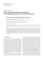
Figure 1: Illustration of the wavelet packet decomposition and the
tree structure for SPIHT. All descendants for a coefficient (i, j, k)
with i and k being odd and j being even are shown.
remote sensing applications as in the case of the international
charter: space and major disasters [3]. Resolution scalability is
necessary to dramatically reduce the bit rate and provide only
the necessary information for the application.
The SPIHT (set partitioning in hierarchical trees) algo-
rithm [4] is a good candidate for onboard hyperspec-
tral data compression. A modified version of SPIHT is
currently flying toward the 67P/Churyumov-Gerasimenko
comet and is targeted to reach in 2014 (Rosetta mission)
among other examples. This modified version of SPIHT
is used to compress the hyperspectral data of the VIRTIS
instrument [5]. This interest is not restricted to hyperspectral

data. The current development of the CCSDS (Consultative
Committee for Space Data Systems, which gathers experts
from different space agencies as NASA, ESA, and CNES) is
oriented toward zerotrees principles [6] because JPEG2000
suffers from implementation difficulties as described in [7]
(in the context of implementation compatible with space
constraints).
Several papers develop the issue of adaptation from 2D
coding to 3D coding using zerotree-based methods. One
example is adaptation to multispectral images in [8] through
a Karhunen-Loeve transform on the spectral dimension and
another is to medical images where [9] uses an adaptation of
the 3D SPIHT, first presented in [10]. In [11], a more efficient
tree structure is defined and a similar structure proved to
be nearly optimal in [12, 13]. To increase the flexibility and
the features available as specified in [14], modifications are
required. The problem of error resilience is developed in [15]
on a block-based version of 3D-SPIHT. A general review of
these modifications and a comparison of performances is
provided in [16]. Few papers focus on the resolution scala-
bility,asisdoneinpapers[10, 17–20], adapting SPIHT or
SPECK (set partitioning-embedded block)[21] algorithms.
However, none offers to differentiate the different directions
along the coordinate axes to allow full spatial resolution with
reduced spectral resolution. In [17, 18], the authors report
a resolution and quality scalable two-dimensional SPIHT,
but without the random access capability to be enabled in
our proposed algorithm. Our proposed extension to three
dimensions with random access decodability that retains
spatial and quality scalability requires significant changes of

the transform and tree structure and search mode, and the
addition of a post-compression rate allocation procedure.
To the authors’ knowledge, no previous work presents the
combination of all these features doing a rate distortion
optimization between blocks, while maintaining optimal
rate-distortion performance and preserving the properties of
spatial and quality scalability.
This paper presents the extension of the well-known
SPIHT algorithm for 3D data enabling random access
and resolution scalability, while keeping quality and rate
scalability and extends the previous work presented in [22].
Compression performance and attributes are compared with
JPEG2000 [23].
2. DATA DECORRELATION AND TREE STRUCTURE
2.1. 3D anisotropic wavelet transform
Hyperspectral images contain one image of the scene for
different wavelengths, thus two dimensions of the 3D
hyperspectral cube are spatial and the third one is spectral (in
the wavelength (λ) sense). Medical magnetic resonance (MR)
or computed tomography (CT) images contain one image for
each slice of observation, in which case the three dimensions
are spatial. However, the resolution and statistical properties
of the third direction are different. To avoid confusion,
the first two dimensions are referred to as spatial, whereas
the third one is called spectral. An anisotropic 3D wavelet
transform is applied to the data for the decorrelation. This
decomposition consists of performing a classic dyadic 2D
wavelet decomposition on each image followed by a 1D
dyadic wavelet decomposition in the third direction. The
obtained subband organization is represented in Figure 1

and is also known as wavelet packet. The decomposition
is nonisotropic as not all subbands are regular cubes and
some directions are privileged. It has been shown that
this anisotropic decomposition is nearly optimal in a rate-
distortion sense in terms of entropy [24]aswellasreal
coding [12]. To the authors’ knowledge, this is valid for
3Dhyperspectraldataaswellasfor3Dmagneticresonance
medical images and video sequences. Moreover, this is the
only 3D wavelet transform supported by the JPEG2000
standard in Part II [25].
2.2. Tree structure
The SPIHT algorithm [4] uses a tree structure to define
a relationship between wavelet coefficients from different
subbands. To adapt the SPIHT algorithm on the anisotropic
3-D (wavelet packet) decomposition, a suitable tree structure
must be defined. Let us define O
spat
(i, j,k) as the spatial
(x
− y band in Figure 1)offspring of the pixel located at
sample i, line j in band k. The first coefficient in the upper
front, left corner is noted as (0, 0, 0). In the spatial direction,
E. Christophe and W. A. Pearlman 3
the relation is similar to the one defined in the original
SPIHT. In general, we have O
spat
(i, j,k) ={(2i,2j, k),(2i +
1, 2j, k), (2i,2j +1,k), (2i+1,2j +1,k)
}. In the highest spatial
frequency subbands, there are no offspring: O

spat
(i, j,k) = ∅.
In the lowest frequency subband, coefficients are grouped in
2
× 2 as in the original SPIHT. Let n
s
denote the number
of samples per line and n
l
the number of lines in the
lowest frequency subband. We have for (i, j,k) in the lowest
frequency subband:
(i) if i even and j even: O
spat
(i, j,k) = ∅;
(ii) if i odd and j even: O
spat
(i, j,k) ={(i +n
s
−1, j, k), (i+
n
s
, j,k), (i + n
s
−1, j +1,k), (i + n
s
, j +1,k)};
(iii) if i even and j odd: O
spat
(i, j,k) ={(i, j +n

l
−1, k), (i +
1, j + n
l
−1, k),(i, j + n
l
, k),(i +1,j + n
l
, k)};
(iv) if i odd and j odd: O
spat
(i, j,k) ={(i + n
s
−1, j + n
l
−
1, k),(i +n
s
, j +n
l
−1, k), (i +n
s
−1, j +n
l
, k),(i +n
s
, j +
n
l
, k)}.

The spectral (λ direction in Figure 1)offspring O
spec
(i,
j, k) are defined in a similar way, but only for the lowest
spatial subband: if i
≥ n
s
or j ≥ n
l
,wehaveO
spec
(i, j,k) = ∅.
Otherwise, apart from the highest and lowest spectral fre-
quency subbands, we have O
spec
(i, j,k) ={(i, j,2k), (i, j,2k+
1)
} for i<n
s
and j<n
l
. In the highest spectral frequency
subbands, there are no offspring: O
spec
(i, j,k) = ∅ and in the
lowest, coefficients are grouped by 2 to have a construction
similar to SPIHT. Let n
b
be the number of spectral bands in
the lowest spectral frequency subband:

(i) if i<n
s
, j<n
l
, k even: O
spec
(i, j,k) = ∅;
(ii) if i<n
s
, j<n
l
, k odd: O
spec
(i, j,k) ={(i, j, k + n
b
−
1), (i, j,k + n
b
)}.
With these relations, we have a separation in nonover-
lapping trees of all the coefficients of the wavelet transform
of the image. The tree structure is illustrated in Figure 1 for
three levels of decomposition in each direction. Each of the
coefficients is the descendant of a root coefficient located
in the lowest frequency subband. It has to be noted that all
the coefficients belonging to the same tree correspond to a
geometrically similar area of the original image, in the three
dimensions.
We can compute the maximum number of coefficients
in a tree rooted at (i, j, k) for a 5 level spatial and spectral

decomposition. The maximum of descendants occurs when
k is odd and at least either i or j is odd. For this situation,
wehave1+2+2
2
+ ···+2
5
= 2
6
− 1 spectral descendants
(including the root) and for each of these, we have 1 + 2
2
+
(2
2
)
2
+(2
3
)
2
+ ···+(2
5
)
2
= 2
0
+2
2
+2
4

+ ···+2
10
= (2
12
−
1)/3 spatially linked coefficients. Let l
spec
be the number of
decompositions in the spectral direction and let l
spac
be the
same in the spatial direction, we obtain the general formula:
n
desc
=

2
l
spec
+1
−1

2
2
(l
spac
+1)
−1
3
(1)

for the maximum number of coefficients in a tree. Thus the
number of coefficients in the tree is at most 85995 (l
spec
= 5
and l
spat
= 5) if the given coefficient has both spectral and
spatial descendants. Coefficient (0, 0, 0), for example, has no
descendants at all.
3. BLOCK CODING
To provide random access, it is necessary to encode separately
different areas of the image. Encoding separately portions
of the image provides several advantages. First, scan-based
mode compression is made possible as the whole image is not
necessary. Once again, we do not consider here the problem
of the scan-based wavelet transform which is a separate
issue. Secondly, encoding parts of the image separately also
provides the ability to use different compression parameters
for different parts of the image, enabling the possibility of
high-quality region of interest (ROI) and the possibility of
discarding unused portions of the image. An unused portion
of the image could be an area with clouds in remote sensing
or irrelevant organs in a medical image. Third, transmission
errors have a more limited effect in the context of separate
coding; the error only affects a limited portion of the image.
Direct transformation and coding different portions of
the image results in poor coding efficiency and blocking
artifacts visible at boundaries between adjacent portions.
However, if we encode portions of the full-image transform
corresponding to image regions that together constitute

the whole, coding efficiency is maintained and boundary
artifacts vanish in the inverse transform process. This
strategy has been used for this particular purpose on the
EZW algorithm in [26], and in [15] for 3D-SPIHT in the
context of video coding. Finally, one limiting factor of the
SPIHT algorithm is the complicated list processing requiring
a large amount of memory. If the processing is done only
on one part of the transform at a time, the number of
coefficients involved is dramatically reduced and so is the
memory necessary to store the control lists in SPIHT.
With the tree structure defined in Section 2,anatu-
ral block organization appears. A tree-block (later simply
referred to as block) is generated by 8 coefficients forming
a2
× 2 × 2 cube from the lowest subband together with
all their descendants. It is more easily visualized in the two-
dimensional case in Figure 2, where is shown a 2
×2groupin
the lowest frequency subband and all its descendants forming
a tree-block. All the coefficients linked to the root coefficient
in the lowest subband shown for three dimensions on
Figure 1 are part of the same tree-block together with seven
other trees. Grouping the coefficients by 8 enables the use of
neighbor similarities between coefficients. This grouping of
coefficients in the lowest frequency subband is analogous to
the grouping of 2
× 2 in the original SPIHT patent [27]and
paper [4]. The gray-shaded coefficients in Figure 1 constitute
a block in our three-dimensional transform.
For this grouping, the number of coefficients in each

block will be the same, the only exception being the case
where at least one dimension of the lowest subband is
odd. In a 2
× 2 × 2 root group, we have three coefficients
which have the full sets of descendants, whose number
is given by (1), three have only spatial descendants, one
has only spectral descendants, and the last one has no
descendant. The number of coefficients in a block, which
4 EURASIP Journal on Image and Video Processing
Figure 2: Equivalence of the block structure for 2D, all coefficients
in gray belong to the same block. In the following algorithm, an
equivalent 3D block structure is used.
determines the maximum amount of memory necessary for
the compression, will finally be 262144
= 2
18
(valid for 5
decompositions in the spatial and spectral directions).
The granularity of the random access obtained with
this method is very small. Spatially, the grain size is 2
×
2, compared to JPEG2000’s 32 × 32 or 64 × 64, which
are the typical sizes of the encoded subblocks of the
subbands. Using subblocks smaller than 32
×32 in JPEG2000
results in considerable loss of coding efficiency. JPEG2000
encodes the spectrally transformed slices or spectral bands
independently, so its grain size in the spectral direction is 1
versus 2 for our method. With the 2
× 2 × 2rootgroup,it

is possible to retrieve almost only the required coefficients
to decode a given area. Moreover, every coefficient can be
retrieved only to the bit plane necessary to give the expected
quality.
4. ENABLING RESOLUTION SCALABILITY
4.1. Original SPIHT algorithm
The original SPIHT algorithm processes the coefficients bit
plane by bit plane. Coefficients are stored in three different
lists according to their significance. The list of significant
pixels (LSP) stores the coefficients that have been found
significant in a previous bit plane and that will be refined
in the following bit planes. Once a coefficient is on the LSP,
it remains significant at all lower thresholds. It stays on the
LSP, so that it can be successively refined with bits from its
lower bit planes. The list of insignificant pixels (LIP) contains
the coefficients which are still insignificant, relative to the
current bit plane and which are not part of a tree from the
third list (LIS). Coefficients in the LIP are transferred to the
LSP when they become significant. The third list is the list
of insignificant sets (LIS). A set is said to be insignificant if
all descendants, in the sense of the previously defined tree
structure, are not significant in the current bit plane. For the
0
1
2
3
5
4
4
4

6
7
8
12
15
14
13
9
10
11
15
14
13
12
8
8
12
13
14
x
y
λ
Figure 3: Illustration of the resolution level numbering. If a low-
resolution image is required (either spectral or spatial), only sub-
bands with a resolution number corresponding to the requirements
are processed.
bit plane t, we define the significance function S
t
of a set T
of coefficients :

S
t
(T ) =
⎧
⎨
⎩
0if∀c ∈ T ,|c|< 2
t
1if∃c ∈ T ,|c|≥2
t
.
(2)
If T consists of a single coefficient, we denote its
significance function by S
t
(i, j,k).
Let D(i, j, k) be all descendants of (i, j,k), O(i, j,k)
only the offspring (i.e., the first-level descendants) and
L(i, j,k)
= D(i, j,k) − O(i, j, k), the granddescendant set.
AtypeAtreeisatreewhereD(i, j, k) is insignificant (all
descendants of (i, j,k) are insignificant); a type B tree is a
tree where L(i, j, k) is insignificant (all granddescendants of
(i, j,k) are insignificant). The full SPIHT algorithm can be
found in [4].
4.2. Introducing resolution scalability
In SPIHT, there is no distinction between coefficients from
different resolution levels. To provide resolution scalability,
we need to provide the ability to decode only the coefficients
from a selected resolution. A resolution comprises 1 or 3

subbands. To enable this capability, we keep three lists for
each resolution level r. When r
= 0, only coefficients from
the low-frequency subbands will be processed. Resolution
levels must be processed in increasing order because to
reconstruct a given resolution, all the lower-order resolution
levels are needed. Coefficients are processed according to
the resolution level to which they correspond. For a 5-level
wavelet decomposition in the spectral and spatial direction,
a total of 36 resolution levels will be available (illustrated
on Figure 3 for 3-level wavelet and 16 resolution levels
available). Each level r keeps in memory three lists: LSP
r
,
LIP
r
,andLIS
r
.
E. Christophe and W. A. Pearlman 5
Some difficulties arise from this organization and the
progression order to follow; several options are available
(Figure 4). If the priority is given to full-resolution scalability
compared to the bit plane scalability, some extra precautions
have to be taken. The different possibilities for scalability
order are discussed in Section 4.3. In the most complicated
case, where all bit planes for a given resolution r are pro-
cessed before the descendant resolution r
d
(full-resolution

scalability), the last element to process for LSP
r
d
,LIP
r
d
,
and
LIS
r
d
for each bit plane t has to be remembered. Details of
the resolution-scalable algorithm, referred as SPIHT RARS
(Random Access with Resolution Scalability) are given in
Algorithm 1.
This new algorithm, which processes all bit planes at a
given resolution level, provides strictly the same code bits
as the original SPIHT. The bits are just organized in a
different order. With the block structure, memory footprint
during compression is dramatically reduced. The resolution
scalability with its several lists does not increase the amount
of memory necessary as the coefficients are just spread onto
different lists.
4.3. Switching loops
The priority of scalability type can be chosen by the progres-
sion order of the two “for” loops (just after the inialization
stage) in the 3D SPIHT RARS algorithm. As written, the
priority is resolution scalability, but these loops can be
inverted to give priority to quality scalability. The different
progression orders are illustrated in Figures 4(a) and 4(b).

Processing the resolution completely before proceeding to
the next one (Figure 4(b)) requires more precautions.
When processing resolution r, a significant descendant
set is partitioned into its offspring in r
d
and its grandde-
scendant set. Therefore, some coefficients are added to LSP
r
d
in the step marked (2) in the algorithm (similar for the
LIP
r
d
and LIS
r
d
). This is an additional step compared to the
original SPIHT [4]. So even before processing resolution r
d
,
the LSP
r
d
may contain some coefficients which were added at
different bit planes. One possible content of an LSP
r
d
could
be
LSP

r
d
={(i
0
, j
0
, k
0
)(t
19
), (i
1
, j
1
, k
1
)(t
19
), ,
(i
n
, j
n
, k
n
)(t
12
), ,
(i
n


, j
n

, k
n

)(t
0
), },
(3)
(the bit plane when a coefficient was added to the list is given
in parentheses following the coordinate) 19 being the highest
bit plane in this case (depending on the image).
When we process LSP
r
d
,
we should skip entries added at
lower bit planes than the current one. For example, there is
no meaning to refine a coefficient added at t
12
when we are
working in bit plane t
18
.
Furthermore, at the step marked (1) in the algorithm
above, when processing resolution r
d
we add some coeffi-

cients to LSP
r
d
. These coefficients have to be added at the
proper position within LSP
r
d
to preserve the order. When
adding a coefficientatstep(1) for the bit plane t
19
, we insert it
just after the other coefficient from bit plane t
19
(at the end of
Resolution
High
frequency
Low
frequency
MSB LSB Bitplane
(a)
Resolution
High
frequency
Low
frequency
MSB LSB Bitplane
(b)
Figure 4: Scanning order for SNR scalability (a) or resolution
scalability (b).

B
k
l
0
l
2
l
1
l
3
R
0
R
1
R
2
···t
19
t
18
t
17
t
19
t
18
t
17
··· t
19

t
18
···
Figure 5: Resolution scalable bitstream structure with header. The
header allows the decoder to jump directly to resolution 1 without
completely decoding or reading resolution 0. R
0
, R
1
, denote the
different resolutions, t
19
, t
18
, the different bit planes. l
i
is the size
in bits of R
i
.
the first line of (3). Keeping the order avoids looking through
the whole list to find the coefficientstoprocessatagivenbit
plane and can be done simply with a pointer.
The bitstream structure obtained for this algorithm is
shown in Figure 5 and is called the resolution scalable
structure. If quality scalability replaces resolution scalability
as a priority, the “for” loops, that step through resolutions
and bit planes, can be inverted to process one bit plane
completely for all resolutions before going to the next bit
plane. In this case, the bitstream structure obtained is

different and illustrated in Figure 6 and is called the quality
6 EURASIP Journal on Image and Video Processing
// Initialization step:
t
← number of bit planes
LSP
0
← ∅
LIP
0
← all the coefficients without any parents (the 8 root
coefficients of the block);
LIS
0
← all coefficients from the LIP
0
with descendants (7
coefficients as only one has no descendant);
For r
/
=0, LSP
r
← ∅,LIP
r
← ∅,LIS
r
← ∅;
// List processing:
for each r from 0 to maximum resolution do
for each t from the highest bit plane to 0(bit planes) do

// Sorting pass:
for each entry (i, j, k) of the LIP
r
which had been
added at a threshold strictly greater to the current t do
Output S
t
(i, j, k);
If S
t
(i, j, k) = 1, move (i, j, k)toLSP
r
and
output the sign of c
i,j,k
(1);
for each entry (i, j, k) of the LIS
r
which had been
added at a threshold greater or equal to the current t
do
if the entry is type A then
Output S
t
(D(i, j, k);
if S
t
(D(i, j, k)) = 1 then
for all (i


, j

, k

) ∈ O(i, j,k) do
output S
t
(i

, j

, k

);
if S
t
(i

, j

, k

) = 1 then
add (i

, j

, k

) to the LSP

r
d
;
Output the sign of c
i

,j

,k

;
else add (i

, j

, k

) to the end of the
LIP
r
d
(2);
if L(i, j, k)
/
=∅ then move (i, j,k)tothe
LIS
r
as a type B entry;
else remove (i, j, k) from the LIS
r

;
if the entry is type B then
Output S
t
(L(i, j, k));
if S
t
(L(i, j, k)) = 1 then
Add all the (i

, j

, k

) ∈ O(i, j,k)tothe
LIS
r
d
as a type A entry;
Remove (i, j, k) from the LIS
r
;
//Refinement pass:
for all e ntries (i, j,k) of the LSP
r
which had been
added at a threshold strictly greater than the current
t do
Output the tth most significant bit of c
i,j,k

Algorithm 1: Resolution scalable 3D SPIHT RARS.
scalable structure. The differences between scanning order
are shown in Figure 4.
4.4. More flexibility at decoding
3D SPIHT RARS possesses great flexibility and the same
image can be encoded up to an arbitrary resolution level or
down to a certain bit plane, depending on the two possible
loop orders. The decoder can just proceed to the same level
to decode the image. However, an interesting feature to have
is the possibility to encode the image only once, with all
resolution and all bit planes and then during the decoding to
choose which resolution and which bit plane to decode. One
may need only a low-resolution image with high-radiometric
precision or a high-resolution portion of the image with
rough-radiometric precision.
When the resolution scalable structure is used (Figure 5),
it is easy to decode up to the desired resolution, but if not
all bit planes are necessary, we need a way to jump to the
beginning of resolution 1 once resolution 0 is decoded for
the necessary bit planes. The problem is the same with the
quality scalable structure (Figure 6) exchanging bit plane and
resolution in the problem description.
E. Christophe and W. A. Pearlman 7
B
k
l
19
l
17
l

18
l
16
t
19
t
18
t
17
R
0
R
1
R
2
···
R
0
R
1
R
2
···
R
0
R
1
···
Figure 6: Quality scalable bitstream structure with header. The
header allows the decoder to continue the decoding of a lower bit

plane without having to finish all the resolution at the current bit
plane. R
0
, R
1
, denote the different resolutions, t
19
, t
18
, the
different bit planes. l
i
is the size in bits of the bit plane corresponding
to t
i
.
To overcome this problem, we need to introduce a block
header describing the size of each portion of the bitstream.
The cost of this header is negligible: the number of bits for
each portion is coded with 24 bits, enough to code part sizes
up to 16 Mbits. The lowest resolutions (resp., the highest bit
planes) which are using only few bits will be processed fully,
regardless of the specification at the decoder, as the cost in
size and processing is low and therefore their sizes need not to
be kept. Only the sizes of long parts are kept: we do not keep
the size individually for the first few bit planes or the first few
resolutions, since they will be decoded in any case. Only the
sizes of lower bit planes and higher resolutions (in general
well above 10000 bits), which comprise about 10 numbers
(each coded with 32 bits to allow sizes up to 4 Gb), need to

be written to the bitstream. Then this header cost will remain
below 0.1%.
As in [17], simple markers could have been used to
identify the beginning of new resolutions of new bit planes.
Markers have the advantage to be shorter than a header
coding the full size of the following block. However, markers
make the full reading of the bitstream compulsory and the
decoder cannot just jump to the desired part. As the cost of
coding the header remains low, this solution is chosen.
5. DRAWBACKS OF BLOCK PROCESSING
AND INTRODUCTION OF RATE ALLOCATION
5.1. Rate allo cation and keeping the SNR scalability
The problem of processing different areas of the image
separately always resides in the rate allocation for each of
these areas. A fixed rate for each area is usually not a suitable
decision as complexity most probably varies across the
image. If quality scalability is necessary for the full image, we
need to provide the most significant bits for one block before
finishing the previous one. This could be obtained by cutting
the bitstream for all blocks and interleaving the parts in the
proper order. With this solution, the rate allocation will not
be available at the bit level due to the block organization
and the spatial separation, but a tradeoff with quality layers
organization can be used.
5.2. Layer organization and rate-distortion
optimization
The idea of quality layers is to provide different targeted bit
rates in the same bitstream [28]. For example, a bitstream can
B
0

λ
0
λ
1
t
19
t
18
t
17
R
0
R
1
R
2
···
R
0
R
1
R
2
···
R
0
R
1
···
B

1
λ
0
λ
1
t
19
t
18
t
17
R
0
R
1
R
2
···
R
0
R
1
R
2
···
R
0
R
1
R

2
···
B
2
λ
0
λ
1
t
19
t
18
t
17
R
0
R
1
R
2
···
R
0
R
1
R
2
···
R
0

R
1
···
Figure 7: An embedded scalable bitstream generated for each block
B
k
. The rate-distortion algorithm selects different cutting points
corresponding to different values of the parameter λ. The final
bitstream is illustrated in Figure 8.
provide two quality layers: one at 1.0 bits per pixel (bpp) and
another at 2.0 bpp. If the decoder needs a 1.0 bpp image, just
the beginning of the bitstream is transferred and decoded. If
a higher-quality image is needed, the first layer is transmitted,
decoded, and then refined with the information from the
second layer.
As the bitstream for each block is already embedded,
to construct these layers, we just need to select the cutting
points for each block and each layer leading to the correct
bit rate with the optimal quality for the entire image. Once
again, it has to be a global optimization and not only local,
as complexity will vary across blocks.
A simple Lagrangian optimization method [29] gives the
optimal cutting point for each block B
k
. This optimization
consists in minimizing the cost function J(λ)
=

k
(D

k
+
λR
k
): D
k
being the distortion of the block B
k
, R
k
its rate,
and λ the Lagrange parameter. This Lagrangian optimization
to find the cutting point between different blocks is also
used in JPEG2000 and referred to as PCRD-opt (post-
compression rate-distortion optimization) [28]. It has to
be noted that the progressive bit plane coding of SPIHT
provides a straightforward implementation of this method.
The result of the Lagrangian optimization led to an
interleaved bitstream between different blocks, as described
in Figures 7 and 8.
5.3. Low-cost distortion tracking:
during the compression
In the previous part, we assumed that the distortion was
known for every cutting point (every bit in fact) of the
bitstream for one block. As the bitstream for one block is
in general about millions of bits, it is too costly to keep all
this distortion information in memory. Only a few hundred
cutting points are recorded with their rate and distortion
information.
Getting the rate for one cutting point is the easy part:

one just has to count the number of bits before this point.
The distortion requires more processing. The distortion
value during the encoding of one block can be obtained
8 EURASIP Journal on Image and Video Processing
Table 1: Data sets.
Image Type Dynamic Size σ
2
Moffett sc1 Hyperspectral 16 bits 512 ×512 × 224 1749626.1
Moffett sc3 Hyperspectral 16 bits 512
×512 ×224 1666647.5
Jasper sc1 Hyperspectral 16 bits 512
×512 ×224 1361347.8
Cuprite sc1 Hyperspectral 16 bits 512
×512 ×224 3212383.2
CT
skull CT 8 bits 256 ×256 ×192 3201.0540
CT
wrist CT 8 bits 256 ×256 ×176 2431.6957
MR
sag head MR 8 bits 256 ×256 ×56 671.58119
MR
ped chest MR 8 bits 256 ×256 ×64 444.34858
l(B
0
, λ
0
)
l(B
1
, λ

0
) l(B
2
, λ
0
) l(B
0
, λ
1
) l(B
1
, λ
1
)
R
0
R
1
R
2
··· R
0
R
0
R
1
R
2
···
R

0
R
1
R
2
R
1
R
2
···
R
0
R
0
R
1
R
2
···
R
0
R
1
R
2
B
0
B
1
B

2
B
0
B
1
Layer 0: λ
0
Layer 1: λ
1
Figure 8: The bitstreams are interleaved for different quality layers. To permit the random access to the different blocks, the length in bits of
each part corresponding to a block B
k
and a quality layer corresponding to λ
q
is given by l(B
k
, λ
q
).
with a simple tracking. Let us consider the instant in the
compression when the encoder is adding one precision bit
for one coefficient c at the bit plane t.Letc
t
denote the new
approximation of c in the bit plane t given by adding this new
bit. c
t+1
was the approximation of c at the previous bit plane.
SPIHT uses a deadzone quantizer, so if the refinement bit
is 0, we have c

t
= c
t+1
− 2
t−1
and if the refinement bit is 1,
we have c
t
= c
t+1
+2
t−1
.LetuscallD
a
the total distortion of
the block after this bit was added and D
b
the total distortion
before. We have the following:
(i) with a refinement bit of 0:
D
a
−D
b
= (c −c
t
)
2
−(c − c
t+1

)
2
=

c
t+1
−c
t
)(2c − c
t
−c
t+1

=
2
t−1

2(c − c
t+1
)+2
t−1

,
(4)
giving
D
a
= D
b
+2

t−1

2(c − c
t+1
)+2
t−1

;(5)
(ii) with a refinement bit of 1:
D
a
= D
b
−2
t−1

2(c − c
t+1
) −2
t−1

. (6)
Since this computation can be done using only right and
left bit shifts and additions, the computational cost is low.
The algorithm does not need to know the initial distortion
value as the rate-distortion method holds if distort ion is
replaced by distortion reduction . The value can be high and
has to be kept internally in a 64-bit integer. As seen before, we
have 2
18

coefficients in one block, and for some of them, the
value can reach 2
20
. Therefore, 64 bits seem to be a reasonable
choice that remains valid for the worst cases.
The evaluation of the distortion is done in the transform
domain, directly on the wavelet coefficients. This can be
done only if the transform is orthogonal. The 9/7 transform
is approximately orthogonal. In [30], the computation of
the weight to apply to each wavelet subband for the rate
allocation is detailed. The weight can be introduced as in (5)
and (6) as a multiplicative factor to get a precise distortion
evaluation in the wavelet domain. However, the gain in
quality introduced by the increase in precision is negligible
(about 0.01 dB) compared to the increase in complexity.
Thus these weights are not kept in the following results.
6. RESULTS
6.1. Data and performance measurement
The hyperspectral data subsets originate from the airborne
visible infrared imaging spectrometer (AVIRIS) sensor. We
use radiance unprocessed data. The original AVIRIS scenes
are 614
× 512 × 224 pixels. For the simulations here, we crop
the data to 512
× 512 × 224 starting from the upper left
corner of the scene. To make comparison easier with other
papers, we use well-known data sets: particularly scenes 1
and3oftherunfromAVIRISonMoffett Field, but also scene
1 over Jasper Ridge and scene 1 over Cuprite site. MR and CT
medical images are also used. The details of all the images are

given in Ta ble 1.
Error is given in terms of signal-to-noise ratio (SNR),
root mean square error (RMSE), and maximum error e
max
.
SNR is computed according to the variance (σ
2
)valuesfrom
Ta ble 1 :SNR
= 10log
10
σ
2
/MSE. All errors are measured
in the final reconstructed dataset compared to the original
data. Choosing a distortion measure suitable to hyperspectral
data is not easy matter as shown in [31]. The rate-distortion
optimization is based on the additive property of the
distortion measure and optimized for the mean squared
error (MSE). Our goal here is to choose an acceptable
E. Christophe and W. A. Pearlman 9
distortion measure for general use on different kinds of
volume images. The MSE-based distortion measures here
are appropriate and popular and are selected to facilitate
comparisons.
Final rate is calculated directly from the size of the
codestream and includes all headers and required side
information. This rate is given in terms of bits per pixel
per band (bpppb), where band means spectral band for
hyperspectral data and axial slice for medical data.

An optional context-based arithmetic coder is included
to improve rate performance [32]. In the context of a
reduced complexity algorithm, the slight improvement in
performance introduced by the arithmetic coder does not
seem worth the complexity increase. Results with arithmetic
coder are given for reference in Ta ble 2 . Unless stated
otherwise, results in this paper do not include the arithmetic
coder. Several particularities have to be taken into account
to preserve the bitstream flexibility. First, contexts of the
arithmetic coder have to be reset at the beginning of each
part to be able to decode the bitstream partially. Secondly, the
rate recorded during the rate-distortion optimization has to
be the rate provided by the arithmetic coder.
The raw compression performances of the previously
defined random access with resolution scalability (3D-
SPIHT-RARS) are compared with the best up to date method
without taking into account the specific properties available
for the previously defined algorithm. The reference results
are obtained with the version 5.0 of Kakadu software [33]
using the JPEG2000 Part 2 options: wavelet intercomponent
transform to obtain a transform similar to the one used
by our algorithm. SNR values are similar to the best values
published in [34]. The results were also confirmed using the
latest reference implementation of JPEG2000, the verification
model (VM) version 9.1. Our results are not expected to be
better, but are here to show that the increase in flexibility does
not come with a prohibitive cost in performance. It also has
to be noted that the results presented here for 3D-SPIHT-
RARS do not include any entropy coding of the SPIHT
sorting output, thus simplifying the implementation.

6.2. Performance comparisons
First, coding results are compared with the original SPIHT.
The decrease in quality is very low at 1 bpppb (under 0.05 dB)
and remain low at 0.5 bpppb (about 0.40 dB). The source
of performance decrease is the separation of the wavelet
subbands at each bit plane which causes different bits to
be kept if the bitstream is truncated. Once again, if lossless
compression is required, the two algorithms, SPIHT and
SPIHT-RARS, provide exactly the same bits reordered (apart
from the headers).
Computational complexity is not easy to measure, but
one way to get a rough estimation is to measure the time
needed for the compression of one image. The version of 3D-
SPIHT here is a demonstration version and there is a lot of
room for improvement. The compression time with similar
options is 20 s for Kakadu v5.0, 600 s for VM 9.1, and 130 s
for 3D-SPIHT-RARS. These values are given only to show
that compression time is reasonable for a demonstration
Table 2: Lossless compression rates (bpppb) (results denoted with
∗
use the additional lifting steps from [9]).
Image JPEG2000 MT SPIHT-RARS SPIHT-RARS
(with AC)
CT skull 2.93 2.21 2.16
CT
wrist 1.78 1.30 1.27
MR
sag head 2.30 2.41 2.35
MR
ped chest 2.00 1.96 1.92

Moffett sc3 5.14 5.37
∗
5.29
∗
Moffett sc1 5.65 5.83
∗
5.75
∗
Jasper sc1 5.55 5.74
∗
5.67
∗
Cuprite sc1 5.29 5.51
∗
5.43
∗
Table 3: Quality for different rates for Moffett sc3.
Rate (bpppb) 2.0 1.0 0.5 0.1
SNR
JPEG2000 MT 54.90 48.63 43.52 33.16
3D-SPIHT-RARS 54.07 47.84 42.49 32.28
RMSE
JPEG2000 MT 2.32 4.78 8.61 28.39
3D-SPIHT-RARS 2.56 5.24 9.69 31.42
e
max
JPEG2000 MT 24 66 157 1085
3D-SPIHT-RARS 37 80 161 1020
implementation and the comparison with the demonstration
implementation of JPEG2000, VM9.1 shows that this is the

case. The value given here for 3D-SPIHT-RARS includes the
30 seconds necessary to perform the 3D wavelet transform
with QccPack.
Ta ble 2 compares the lossless performance of the two
algorithms. JPEG2000 is used with a multicomponent trans-
form (MT). For both, the same integer 5/3 wavelet transform
is performed with the same number of decompositions in
each direction. The modified 5/3 wavelet with additional
lifting steps from [9] is also compared.
Performances between the algorithms are quite similar
for the MR images. SPIHT-RARS outperforms JPEG2000
on the CT images, but JPEG2000 gives a lower bit rate for
hyperspectral images. It has to be noted that the original
5/3 wavelet transform gives better results for the medical
images while the modified transform performs better on
hyperspectral images.
Ta ble 3 compares the lossy performances of the two
algorithms in terms of different quality criteria and Ta ble 4
provides the SNR obtained on several popular datasets to
facilitate comparisons. It is confirmed that the increase in
flexibility of the 3D-SPIHT-RARS algorithm does not come
with a prohibitive impact on performances. We can observe
less than 1 dB difference between the two algorithms. A
noncontextual arithmetic coder applied directly on the 3D-
SPIHT-RARS bitstream already reduces this difference to
0.4 dB (not used in the presented results).
6.3. Resolution scalability from a single bitstream
Different resolutions and different quality levels can be
retrieved from one bitstream. Ta ble 5 presents different
10 EURASIP Journal on Image and Video Processing

Table 4: SNR for popular data sets.
Rate (bpppb) 2.0 1.0 0.5 0.1
Moffett sc1
JPEG2000 MT 51.99 45.48 40.18 29.75
3D-SPIHT-RARS 50.87 44.27 39.32 28.82
Jasper sc1
JPEG2000 MT 51.60 44.85 39.31 28.99
3D-SPIHT-RARS 50.52 43.55 38.34 28.03
Cuprite sc1
JPEG2000 MT 56.72 50.99 46.71 38.72
3D-SPIHT-RARS 55.35 50.15 46.04 37.98
CT
skull
(a)
JPEG2000 MT — 39.15 33.23 23.02
3D-SPIHT-RARS — 37.63 31.92 22.39
MR
sag head
(b)
JPEG2000 MT — 33.08 27.53 19.04
3D-SPIHT-RARS — 31.91 26.60 18.45
(a)
PSNR values can be obtained by adding 13.08
(b)
PSNR values can be obtained by adding 19.85
results on Moffett Field scene 3 changing the number of
resolutions and bit planes to decode the bitstream. The
compression is done only once and the final bitstream is
organized in different parts corresponding to different res-
olution and quality. From this single-compressed bitstream,

all these results are obtained by changing the decoding
parameters. Different bit depths and different resolutions are
chosen arbitrarily to obtain a lower resolution and lower
quality image. Distortion measures are provided for the
lower resolution image as well as the bit rate necessary to
transmit or store this image.
For the results presented in Table 5 , similar resolutions
are chosen for spectral and spatial directions, but this is
not mandatory as illustrated in Figure 9. The reference low-
resolution image is the low-frequency subband of the wavelet
transform up to the desired level. To provide an accurate
radiance value, coefficients are scaled properly to compensate
gains due to the wavelet filters (depending on the resolution
level).
Ta ble 5 shows, for example, that discarding the 6 lower
bit planes, a half resolution image can be obtained with
a bit rate of 0.203 bpppb and an RMSE of 6.47 (for this
resolution).
We can see that at high quality, decoding to lower
resolution greatly decreases the retrieval time. An algorithm
working with hyperspectral data could choose to discard 4
bit planes and to work at 1/4 resolution, thereby reducing
the amount of data to process by a factor of 10, and enabling
simple onboard processing while keeping a good spectral
quality (detection of area of interest, detect the clouds to
discard useless information, etc.).
In Figure 9,wecanseedifferent hyperspectral cubes
extracted from the same bitstream with different spatial
and spectral resolutions. The face of the cube is a color
composition from different subbands. The spectral bands

chosen for the color composition in the subresolution
cube correspond to those of the original cube. Some slight
differences from the original cube can be observed on the
subresolution one, due to weighted averages from wavelet
transform filtering spanning contiguous bands.
(a) (b) (c)
(d)
Figure 9: Example of hyperspectral cube with different spectral
and spatial resolution decoded from the same bitstream. (a) is the
original hyperspectral cube. (b) is 1/4 for spectral resolution and
1/4 for spatial resolution. (c) is full spectral resolution and 1/4
spatial resolution. (d) is full spatial resolution and 1/8spectral
resolution.
6.4. ROI coding and selected decoding
The main interest of the present algorithm is in its flexibility.
The bitstream obtained in the resolution scalable mode can
be decoded at variable spectral and spatial resolutions for
each data block. This is done reading, or transmitting, a
minimum number of bits. Any area of the image can be
decoded up to any spatial resolution, any spectral resolution
and any bit plane. This property is illustrated in Figure 10.
Most of the image background (area 1) is decoded at low
spatial and spectral resolutions, dramatically reducing the
amount of bits. Some specific areas are more detailed and,
offer the full spectral resolution (area 2), the full spatial
resolution (area 3), or both (area 4). The image from
Figure 10 was obtained reading only 16907 bits from the
311598 bits belonging to the full codestream.
The region of interest can also be selected during the
encoding while adjusting the number of bit planes to be

encoded for a specific block. In the context of onboard
processing, it would enable further reduction of the bit
rate. The present encoder provides all these capabilities. For
example, an external clouds detection loop could be added
to adjust the compression parameter to reduce the resolution
when clouds are detected. This would decrease the bit rate on
these parts.
7. CONCLUSION
We have presented the 3D-SPIHT-RARS algorithm, an
original extension of the 3D-SPIHT algorithm. This new
algorithm enables resolution scalability for spatial and
E. Christophe and W. A. Pearlman 11
Table 5: Bits read from full codestream for different resolution and quality for moffett3 image.
Number of non decoded bit planes: 0 Number of non decoded bit planes: 2 Number of non decoded bit planes: 4
Resolution Full 1/2 1/4 1/8 Full 1/2 1/4 1/8 Full 1/2 1/4 1/8
bpppb read 5.309 1.569 0.247 0.038 2.857 0.989 0.198 0.033 1.016 0.475 0.132 0.027
RMSE 0.31 0.34 0.25 0.12 1.67 0.70 0.39 0.22 5.18 2.03 0.82 0.44
Time (s) 59.43 21.82 7.17 3.54 42.33 18.03 6.86 3.62 18.18 10.05 5.34 3.45
Number of non decoded bit planes: 6 Number of non decoded bit planes: 8 Number of non decoded bit planes: 10
Resolution Full 1/2 1/4 1/8 Full 1/2 1/4 1/8 Full 1/2 1/4 1/8
bpppb read 0.327 0.203 0.079 0.020 0.104 0.077 0.039 0.013 0.030 0.025 0.016 0.007
RMSE 13.05 6.47 2.73 1.08 30.23 18.97 9.53 3.98 69.41 49.76 29.92 14.60
Time (s) 7.70 6.14 4.40 3.36 4.51 4.26 3.68 3.26 3.47 3.45 3.29 3.16
200150100500
Bands
0
1000
2000
3000
4000

Radiance
(c)Spectrumfrom2
200150100500
Bands
(b)Spectrumfrom1
0
1000
2000
3000
4000
5000
Radiance
200150100500
Bands
(e)Spectrumfrom4
0
2000
4000
6000
Radiance
20015010050 0
Bands
(d)Spectrumfrom3
0
1000
2000
3000
4000
Radiance
1

2
3
4
(a)
Figure 10: Example of a decompressed image with different spatial and spectral resolution for different areas. Background (area 1) is with
low spatial resolution and low spectral resolution as is can be seen on the spectrum (b). Area 2 has low spatial resolution and high spectral
resolution (c), area 3 has high spatial resolution, but low spectral resolution (d). Finally, area 4 has both high spectral and spatial resolutions.
This decompressed image was obtained from a generic bitstream, reading the minimum amount of bits.
spectral dimensions independently and random access
decoding. These properties are important to ease of access
and processing of the data and were not introduced into
SPIHT previously. Coding different areas of the image
transform separately enable random access and region of
interest coding with a reduction in memory usage during
the compression. Furthermore, quality scalability for any
resolution and area can be enabled by reorganization of
the codestream. Thanks to the rate-distortion optimization
between the different blocks, all these features are obtained
without sacrificing compression performance. Most of these
features seem also possible with the JPEG2000 standard.
However, implementation providing multiresolution trans-
formsisveryrecentanddoesnotprovideyetalltheflexibility
proposed here, particularly on the spectral direction. The
granularity of the access is also finer with the proposed
implementation.
The use of an arithmetic coder slightly increases com-
pression performance, but at the cost of an increase in the
complexity. It has to be highlighted that the 3D-SPIHT-
RARS algorithm does not need to rely on arithmetic coding
to obtain competitive results to JPEG2000.

ACKNOWLEDGMENTS
This work has been carried out primarily at Rensselaer
Polytechnic Institute under the financial support of Centre
National d’
´
Etudes Spatiales (CNES), TeSA, Office National
d’
´
Etudes et de Recherches A
´
erospatiales (ONERA), and Alcatel
Alenia Space. Partial support was also provided by the
Office of Naval Research under Award no. N0014-05-10507.
The authors wish to thank their supporters and NASA/JPL
for providing the hyperspectral images used during the
experiments.
12 EURASIP Journal on Image and Video Processing
REFERENCES
[1] S. Krishnamachari and R. Chellappa, “Multiresolution Gauss-
Markov random field models for texture segmentation,” IEEE
Transactions on Image Processing, vol. 6, no. 2, pp. 251–267,
1997.
[2] L. M. Bruce, C. Morgan, and S. Larsen, “Automated detection
of subpixel hyperspectral targets with continuous and discrete
wavelet transforms,” IEEE Transactions on Geoscience and
Remote Sensing, vol. 39, no. 10, pp. 2217–2226, 2001.
[3] “International charter: space and major disasters,” http://
www.disasterscharter.org/main
e.html.
[4] A. Said and W. A. Pearlman, “A new, fast, and efficient image

codec based on set partitioning in hierarchical trees,” IEEE
Transactions on Circuits and Systems for Video Technology, vol.
6, no. 3, pp. 243–250, 1996.
[5] Y. Langevin and O. Forni, “Image and spectral image compres-
sion for four experiments on the ROSETTA and Mars Express
missions of ESA,” in Applications of Digital Image Processing
XXIII, vol. 4115 of Proceedings of SPIE, pp. 364–373, San
Diego, Calif, USA, July 2000.
[6] P S. Yeh, P. Armbraster, A. Kiely, et al., “The new CCSDS
image compression recommendation,” in Proceedings of the
IEEE Aerospace Conference, pp. 4138–4145, Big Sky, Mont,
USA, March 2005.
[7] D. Van Buren, “A high-rate JPEG2000 compression system for
space,” in Proceedings of the IEEE Aerospace Conference,pp.1–
7, Big Sky, Mont, USA, March 2005.
[8] P. L. Dragotti, G. Poggi, and A. R. P. Ragozini, “Compression
of multispectral images by three-dimensional SPIHT algo-
rithm,” IEEE Transactions on Geoscience and Remote Sensing,
vol. 38, no. 1, pp. 416–428, 2000.
[9] Z. Xiong, X. Wu, S. Cheng, and J. Hua, “Lossy-to-lossless com-
pression of medical volumetric data using three-dimensional
integer wavelet transforms,” IEEE Transactions on Medical
Imaging, vol. 22, no. 3, pp. 459–470, 2003.
[10] B J. Kim, Z. Xiong, and W. A. Pearlman, “Low bit-rate
scalable video coding with 3-D set partitioning in hierarchical
trees (3-D SPIHT),” IEEE Transactions on Circuits and Systems
for Video Technology, vol. 10, no. 8, pp. 1374–1387, 2000.
[11]C.He,J.Dong,Y.F.Zheng,andZ.Gao,“Optimal3-D
coefficient tree structure for 3-D wavelet video coding,” IEEE
Transactions on Circuits and Systems for Video Technology, vol.

13, no. 10, pp. 961–972, 2003.
[12] E. Christophe, C. Mailhes, and P. Duhamel, “Hyperspectral
image compression: adapting SPIHT and EZW to anisotropic
3D wavelet coding,” under review IEEE Transactions on Image
Processing.
[13] E. Christophe, C. Mailhes, and P. Duhamel, “Best Anisotropic
3-D wavelet decomposition in a rate-distortion sense,” in
Proceedings of IEEE International Conference on Acoustics,
Speech, and Signal Processing (ICASSP ’06), vol. 1, pp. 17–20,
Toulouse, France, May 2006.
[14] W. A. Pearlman, “Trends of tree-based, set-partitioning com-
pression techniques in still and moving image systems,” in
Proceedings of the 22nd Picture Coding Symposium (PCS ’01),
pp. 1–8, Seoul, Korea, April 2001.
[15] S. Cho and W. A. Pearlman, “Multilayered protection of
embedded video bitstreams over binary symmetric and packet
erasure channels,” Journal of Visual Communication and Image
Representation, vol. 16, no. 3, pp. 359–378, 2005.
[16] J. E. Fowler and J. T. Rucker, “3D wavelet-based compression
of hyperspectral imagery,” in Hyperspectral Data Exploitation:
Theory and Applications, C I. Chang, Ed., pp. 379–407,
chapter 14, John Wiley & Sons, Hoboken, NJ, USA, 2007.
[17] H. Danyali and A. Mertins, “Fully spatial and SNR scalable,
SPIHT-based image coding for transmission over heteroge-
neous networks,” Journal of Telecommunications and Informa-
tion Technology, vol. 2, pp. 92–98, 2003.
[18] H. Danyali and A. Mertins, “Flexible, highly scalable, object-
based wavelet image compression algorithm for network
applications,” IEE Proceedings: Vision, Image, and Signal
Processing, vol. 151, no. 6, pp. 498–510, 2004.

[19] X. Tang and W. A. Pearlman, “Scalable hyperspectral image
coding,” in Proceedings of IEEE International Conference on
Acoustics, Speech, and Signal Processing (ICASSP ’05), vol. 2,
pp. 401–404, Philadelphia, Pa, USA, March 2005.
[20] Y. Cho, W. A. Pearlman, and A. Said, “Low complexity
resolution progressive image coding algorithm: progres (pro-
gressive resolution decompression),” in
Proceedings of IEEE
International Conference on Image Processing (ICIP ’05), vol. 3,
pp. 49–52, Genova, Italy, September 2005.
[21] W. A. Pearlman, A. Islam, N. Nagaraj, and A. Said, “Efficient,
low-complexity image coding with a set-partitionning embed-
ded block coder,” IEEE Transactions on Circuits and Systems for
Video Technology, vol. 14, no. 11, pp. 1219–1235, 2004.
[22] E. Christophe and W. A. Pearlman, “Three-dimensional
SPIHT coding of hyperspectral images with random access
and resolution scalability,” in Proceedings of the 40th Annual
Asilomar Conference on Signals, Systems and Computers,pp.
1897–1901, Pacific Grove, Calif, USA, October-November
2006.
[23] D. S. Taubman and M. W. Marcellin, JPEG2000 Image
Compression Fundamentals, Standards and Practice,Kluwer
Academic Publishers, Boston, Mass, USA, 2002.
[24] B. Penna, T. Tillo, E. Magli, and G. Olmo, “Progressive 3-
D coding of hyperspectral images based on JPEG2000,” IEEE
Geoscience and Remote Sensing Letters, vol. 3, no. 1, pp. 125–
129, 2006.
[25] “Information technology—JPEG2000 image coding system:
extensions,” 2004, ISO/IEC Std. 15 444-2.
[26] C. D. Creusere, “A new method of robust image compression

based on the embedded zerotree wavelet algorithm,” IEEE
Transactions on Image Processing, vol. 6, no. 10, pp. 1436–1442,
1997.
[27] W. A. Pearlman and A. Said, “Data compression using set
partitioning in hierarchical trees,” June 1998, United States
Patent 5,764,807.
[28] D. Taubman, “High performance scalable image compression
with EBCOT,” IEEE Transactions on Image Processing, vol. 9,
no. 7, pp. 1158–1170, 2000.
[29] Y. Shoham and A. Gersho, “Efficient bit allocation for an
arbitrary set of quantizers,” IEEE Transactions on Acoustics,
Speech, and Signal Processing, vol. 36, no. 9, pp. 1445–1453,
1988.
[30] B. Usevitch, “Optimal bit allocation for biorthogonal wavelet
coding,” in Proceedings of the Data Compression Conference
(DCC ’96), pp. 387–395, Snowbird, Utah, USA, March-April
1996.
[31] E. Christophe, D. L
´
eger, and C. Mailhes, “Quality criteria
benchmark for hyperspectral imagery,” IEEE Transactions on
Geoscience and Remote Sensing, vol. 43, no. 9, pp. 2103–2114,
2005.
[32] J. E. Fowler, “QccPack—Quantization, Compression, and
Coding Library,” 2006, />E. Christophe and W. A. Pearlman 13
[33] D. Taubman, “Kakadu Software v 5.0,” 2006, http://www
.kakadusoftware.com/.
[34] J. T. Rucker, J. E. Fowler, and N. H. Younan, “JPEG2000
coding strategies for hyperspectral data,” in Proceedings of
IEEE International Geoscience and Remote Sensing Symposium

(IGARSS ’05), vol. 1, pp. 128–131, Seoul, Korea, July 2005.