Evapotranspiration Remote Sensing and Modeling Part 14 potx

Modelling Evapotranspiration and the Surface Energy Budget in Alpine Catchments 3
Fig. 1. Scheme of the solar radiation components.
where ω is the solid angle seen from the point considered.
The presence of shadows due to surrounding mountains can be expressed through a factor
sw, a function of topography and sun position, defined as:
sw
=

1 if the point is in the sun
0 if the point is in the shadow
(5)
All direct radiation terms have to be multiplied by this factor.
In the next paragraphs we analyze in detail the parametrization of the single terms composing
the radiation flux.
2.1.1 Direct radiation R ↓
SW P
and R ↓
LW P
The direct long-wave radiation R ↓
LW P
is emitted directly by the sun and therefore it is
negligible at the soil level (differently from the long-wave diffuse radiation).
Usually the short-wave radiation R
↓
SW P
is assumed as an input variable, measured or
calculated by an atmospheric model. The direct radiation can be written as the product of
the extraterrestrial radiation R
Extr
by an attenuation factor varying in time and space.
R

↓
SW P
= F
att
R
Extr
(6)
The extraterrestrial radiation can be easily calculated on the basis of geometric formulas
(Iqbal, 1983). The atmospheric attenuation is due to Rayleigh diffusion, to the absorption
on behalf of ozone and water vapor, to the extinction (both diffusion and absorption) due to
atmospheric dust and shielding caused by the possible cloud cover. Moreover the absorption
entity depends on the ray path length through the atmosphere, a function of the incidence
angle and of the measurement point elevation. The effect of the latter can be very important
in a mountain environment, where it is necessary to consider the shading effects.
Part of the dispersed radiation is then returned as short-wave diffuse radiation (R
↓
SW D
) and
part of the energy absorbed by atmosphere is then re-emitted as long-wave diffuse radiation
(R
↓
LW D
).
From a practical point of view, according to the application type and depending on the
measured data possessed, the attenuation coefficient can be calculated with different degrees
of complexity. The radiation transfer through the atmosphere is a well studied phenomenon
379
Modelling Evapotranspiration and the Surface Energy Budget in Alpine Catchments
4 Will-be-set-by-IN-TECH
and there exist many models providing the soil incident radiation spectrum in a detailed way,

considering the various attenuation effects separately (Kondratyev, 1969).
2.1.2 Diffuse downward short-wave radiation R ↓
SW D
This term is a function of the atmospheric radiation due to Rayleigh dispersion and to the
aereosols dispersion, as well as to the presence of cloud cover. The R
↓
SW D
actually is not
isotropic and it depends on the sun position above the horizon. For its parametrization, see,
for example, Paltrige & Platt (1976).
2.1.3 Diffuse downward long-wave radiation R ↓
LW D
Often this term in not provided by standard meteorological measurements, and many LSMs
provide expressions to calculate it. This term indicates the long-wave radiation emitted
by atmosphere towards the earth. It can be calculated starting from the knowledge of the
distribution of temperature, humidity and carbon dioxide of the air column above. If this
information is not available, various formulas, based only on ground measurements, can be
found in literature with expressions as follows:
R
↓
LW D
= 
a
σT
4
a
(7)
with:
T
a

air temperature [K];

a
atmosphere emissivity f (e
a
, T
a
, cloud cover);
e
a
vapor pressure [mb];
Usually for 
a
empirical formulas have been used, but it is also possible to provide a derivation
based on physical topics like in Prata (1996). The cloud cover effect on this term is significant
and not easy to consider in a simple way. Cloud cover data can be provided during the day
by ground or satellite observations but, especially on night, is difficult to collect.
2.1.4 Reflected short-wave radiation R ↑
SW
This term indicates the short-wave energy reflection.
R
↑
SW
= a(R ↓
SW P
+R ↓
SW D
) (8)
where a is the albedo.
The albedo depends strongly on the wave length, but generally a mean value is used for

the whole visible spectrum. Besides its dependance on the surface type, it is important to
consider its dependence on soil water content, vegetation state and surface roughness. The
albedo depends moreover on the sun rays inclination, in particular for smooth surfaces: for
small angles it increases. There is very rich literature about albedo description, it being a key
parameter in the radiative exchange models, see for example Kondratyev (1969). Albedo is
often divided in visible, near infrared, direct and diffuse albedo, as in Bonan (1996).
2.1.5 Long-wave radiation emitted by the surface R ↑
LW
This term indicates the long-wave radiation emitted by the earth surface, considered as a grey
body with emissivity ε
s
(values from 0.95 to 0.98). The surface temperature T
s
[K] is unknown
380
Evapotranspiration – Remote Sensing and Modeling
Modelling Evapotranspiration and the Surface Energy Budget in Alpine Catchments 5
and must be calculated by a LSM. σ = 5.6704 · 10
−8
W/(m
2
K
4
) is Stefan-Boltzman constant.
R
↑
LW
= ε
s
σT

4
s
(9)
2.1.6 Reflected long-wave radiation R ↑
LW R
This term is small and can be subtracted by the incoming long-wave radiation, assuming
surface emissivity ε
s
equal to surface absorptivity:
R
↓
LW D
= ε
s
· 
a
σT
4
a
(10)
2.1.7 Radiation emitted and reflected by surrounding surfaces R ↓
SW O
+R ↓
LW O
It indicates the radiation reflected (R ↑
SW
+R ↑
LW R
) and emitted (R ↑
LW

) by the surfaces
adjacent to the point considered. This term is important at small scale, in the presence of
artificial obstructions or in the case of a very uneven orography. To calculate it with precision it
is necessary to consider reciprocal orientation, illumination, emissivity and the albedo of every
element, through a recurring procedure (Helbig et al., 2009). A simple solution is proposed
for example in Bertoldi et al. (2005).
If the intervisible surfaces are hypothesized to be in radiative equilibrium, i.e. they absorb as
much as they emit, these terms can be quantified in a simplified way:
R
↓
SW O
=(1 − V)R ↑
SW
R ↓
LW O
=(1 − V)( R ↑
LW
+R ↑
LW R
)
(11)
2.1.8 Net radiation
Inserting expressions (7) and ( 9) in the (3), the net radiation is:
R
n
=[sw · R ↓
SW P
+V · R ↓
SW D
](1 − V · a)+V · ε

s
· ε
a
· σ · T
4
a
− V · ε
s
· σ · T
4
s
(12)
with ε
a
= f (e
a
, T
a
, cloud cover) as for example in Brutsaert (1975).
Equation (12) is not invariant with respect to the spatial scale of integration: indeed it contains
non-linear terms in T
a
, T
s
, e
a
, consequently the same results are not obtained if the local values
of these quantities are substituted by the mean values of a certain surface. Therefore, the shift
from a treatment valid at local level to a distributed model valid over a certain spatial scale
must be done with a certain caution.

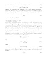
2.1.9 Radiation adsorption and backscattering by vegetation
Expression (12) needs to be modified to take into account the radiation adsorption and
backscattering by vegetation, as shown in Figure 2. This effect is very important to obtain
a correct soil surface skin temperature (Deardorff, 1978). From Best (1998) it is possible to
derive the following relationship:
R
n
=[sw · R ↓
SW P
+V · R ↓
SW D
](1 − V · a) ∗ ( f
trasm
+ a
v
)
+(
1 − ε
v
) · V · ε
s
· ε
a
· σ · T
4
a
+ ε
v
· ε
s

· σ · T
4
v
(13)
where T
v
is vegetation temperature, ε
v
vegetation emissivity (supposed equal to absorption),
a
v
vegetation albedo (downward albedo supposed equal to upward albedo) and f
trasm
381
Modelling Evapotranspiration and the Surface Energy Budget in Alpine Catchments
6 Will-be-set-by-IN-TECH
vegetation transmissivity, depending on plant type, leaf area index and photosynthetic
activity.
Models oriented versus ecological applications have a very detailed parametrization of this
term (Dickinson et al., 1986). Bonan (1996) uses a two-layers canopy model. Law et al. (1999)
explicit the relationship between leaf area distribution and radiative transfer. A first energy
budget is made at the canopy cover layer, and the energy fluxes are solved to find the canopy
temperature, then a second energy budget is made at the soil surface. Usually a fraction of the
grid cell is supposed covered by canopy and another fraction by bare ground.
Shortwave Longwave
Canopy
Ground
Tv
Ts
Veg ads

R↓
↓
SW atm
a
v
R
↓
SW
R
↓
LW
atm
a
v
R
↓
SW
f
trasm
R
↓
SW
a
g
(f
trasm +
a
v
) R
↓

SW
(1-
ε
v
)R
↑
LW
+
ε
v
σ
T
v
4
R
↓
LW
= (1-
ε
v
)R
↓
LW
+
ε
v
σ
T
v
4

R
↑
LW
=
ε
g
σ
T
g
4
+ (1-
ε
g
)R
↓
LW
Fig. 2. Schematic diagram of short-wave radiation (left) and long-wave radiation (right)
absorbed, transmitted and reflected by vegetation and ground , as in equation 13 (from
Bonan (1996), modified).
2.2 Soil heat flux
The soil heat flux G at a certain depth z depends on the temperature gradient as follows:
G = −λ
s
∂T
s
∂z
(14)
where λ
s
is the soil thermal conductivity (λ

s
= ρ
s
c
s
κ
s
with ρ
s
density, c
s
specific heat and κ
s
soil thermal diffusivity) depending strongly on the soil saturation degree. The heat transfer
inside the soil can be described in first approximation with Fourier conduction law:
∂T
s
∂t
= κ
s
∂
2
T
s
∂z
2
(15)
382
Evapotranspiration – Remote Sensing and Modeling
Modelling Evapotranspiration and the Surface Energy Budget in Alpine Catchments 7

Equation (14) neglects the heat associated to the vapor transportation due to a vertical gradient
of the soil humidity content as well as the horizontal heat conduction in the soil. The vapor
transportation can be important in the case of dry climates (Saravanapavan & Salvucci, 2000).
The soil heat flux can be calculated with different degrees of complexity. The most simple
assumption (common in weather forecast models) is to calculate G as a fraction of net radiation
(Stull (1988) suggests G
= 0.1R
n
). Another simple approach is to use the analytical solution for
a sinusoidal temperature wave. A compromise between precision and computational work is
the force restore method (Deardorff, 1978; Montaldo & Albertson, 2001), still used in many
hydrological models (Mengelkamp et al., 1999). The main advantage is that only two soil
layers have to be defined: a surface thin layer, and a layer getting down to a depth where
the daily flux is almost zero. The method uses some results of the analytical solution for
a sinusoidal forcing and therefore, in the case of days with irregular temperature trend, it
provides less precise results.
The most general solution is the finite difference integration of the soil heat equation
in a multilayered soil model (Daamen & Simmonds, 1997). However, this method is
computationally demanding and it requires short time steps to assure numerical stability,
given the non-linearity and stationarity of the surface energy budget, which is the upper
boundary condition of the equation.
2.2.1 Snowmelt and freezing soil
In mountain environments snow-melt and freezing soil should be solved at the same time
as soil heat flux. A simple snow melt model is presented in Zanotti et al. (2004), which has
a lumped approach, using as state variable the internal energy of the snow-pack and of the
first layer of soil. Other models consider a multi-layer parametrization of the snowpack (e.g.
Bartelt & Lehning, 2002; Endrizzi et al., 2006). Snow interception by canopy is described for
example in Bonan (1996). A state of the art freezing soil modeling approach can be found in
Dall’Amico (2010) and Dall’Amico et al. (2011).
2.3 Turbulent fluxes

A modeling of the ground heat and vapor fluxes cannot leave out of consideration the
schematization of the atmospheric boundary layer (ABL), meant as the lower part of
atmosphere where the earth surface properties influence directly the characteristics of the
motion, which is turbulent. For a review see Brutsaert (1982); Garratt (1992); Stull (1988).
A flux of a passive tracer x in a turbulent field (as for example heat and vapor close to the
ground), averaged on a suitable time interval, is composed of three terms: the first indicates
the transportation due to the mean motion v, the second the turbulent transportation
x

v

, the
third the molecular diffusion k.
F = x v + x

v

− k∇x (16)
The fluxes parametrization used in LSMs usually only considers as significant the turbulent
term only. The molecular flux is not negligible only in the few centimeters close the surface,
and the horizontal homogeneity hypothesis makes negligible the convective term.
383
Modelling Evapotranspiration and the Surface Energy Budget in Alpine Catchments
8 Will-be-set-by-IN-TECH
2.3.1 The conservation equations
The first approximation done by all hydrological and LSMs in dealing with turbulent fluxes
is considering the Atmospheric Boundary Layer (ABL) as subject to a stationary, uniform
motion, parallel to a plane surface.
This assumption can become limitative if the grid size becomes comparable to the vertical
heterogeneity scale (for example for a grid of 10 m and a canopy height of 10 m). In this

situation horizontal turbulent fluxes become relevant. A possible approach is the Large Eddy
Simulation (Albertson et al., 2001).
If previous assumptions are made, then the conservation equations assume the form:
• Specific humidity conservation, failing moisture sources and phase transitions:
k
v
∂
2
q
∂z
2
−
∂
∂z
(w

q

)=0 (17)
where:
k
v
is the vapor molecular diffusion coefficient [m
2
/s]
q
=
m
v
m

v
+m
d
is the specific humidity [vapor mass out of humid air mass].
• Energy conservation:
k
h
∂
2
θ
∂z
2
−
∂
∂z
(w

θ

) −
1
ρc
p
∂H
R
∂z
= 0 (18)
where:
k
h

is the thermal diffusivity [m
2
/s]
H
R
is the radiative flux [W/m
2
]
θ is the potential temperature [K]
ρ is the air density [kg/m
3
]
w is the vertical velocity [m/s].
• The horizontal mean motion equations are obtained from the momentum conservation by
simplifying Reynolds equations (Stull, 1988; Brutsaert, 1982 cap.3):
−
1
ρ
∂
p
∂x
+ 2ω sin φ v + ν
∂
2
u
∂z
2
−
∂
∂z

(w

u

)=0 (19)
−
1
ρ
∂
p
∂y
− 2ω sin φ u + ν
∂
2
v
∂z
2
−
∂
∂z
(w

v

)=0 (20)
where:
ν is the kinematic viscosity [m
2
/s]
ω is the earth angular rotation velocity [rad/s]

φ is the latitude [rad] .
The vertical motion equation can be reduced to the hydrostatic equation:
∂p
∂z
= −ρg. (21)
In a turbulent motion the molecular transportation terms of the momentum, heat and vapor
quantity, respectively ν, k
h
and k
v
, are several orders of magnitude smaller than Reynolds
fluxes and can be neglected.
384
Evapotranspiration – Remote Sensing and Modeling
Modelling Evapotranspiration and the Surface Energy Budget in Alpine Catchments 9
2.3.2 Wind, heat and vapor profile at the surface
Inside the ABL we can consider, with a good approximation, that the decrease in the fluxes
intensity is linear with elevation. This means that in the first meters of the air column the
fluxes and the friction velocity u
∗
can be considered constant. Considering the momentum
flux constant with elevation implies that also the wind direction does not change with
elevation (in the layer closest to the soil, where the geostrofic forcing is negligible). In this
way the alignment with the mean motion allows the use of only one component for the
velocity vector, and the problem of mean quantities on uniform terrain becomes essentially
one-dimensional, as these become functions of the only elevation z.
In the first centimeters of air the energy transportation is dominated by the molecular
diffusion. Close to the soil there can be very strong temperature gradients, for example during
a hot summer day. Soil can warm up much more quickly than air. The air temperature
diminishes very rapidly through a very thin layer called micro layer, where the molecular

processes are dominant. The strong ground gradients support the molecular conduction,
while the gradients in the remaining part of the surface layer drive the turbulent diffusion.
In the remaining part of the surface layer the potential temperature diminishes slowly with
elevation.
The effective turbulent flux in the interface sublayer is the sum of molecular and turbulent
fluxes. At the surface, where there is no perceptible turbulent flux, the effective flux is equal to
the molecular one, and above the first cm the molecular contribution is neglegible. According
to Stull (1988), the turbulent flux measured at a standard height of 2 m provides a good
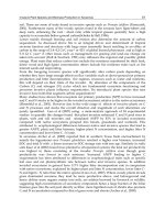
approximation of the effective ground turbulent flux.
Fig. 3. (a) The effective turbulent flux in diurnal convective conditions can be different from
zero on the surface. (b) The effective flux is the sum of the turbulent flux and the molecular
flux (from Stull, 1988).
Applying the concept of effective turbulent flux, the molecular diffusion term can be
neglected, while the hypothesis of uniform and stationary limit layer leads to neglect the
convective terms due to the mean vertical motion and the horizontal flux. The vertical flux at
the surface can then be reduced to the turbulent term only:
F
z
= x

w

(22)
385
Modelling Evapotranspiration and the Surface Energy Budget in Alpine Catchments
10 Will-be-set-by-IN-TECH
In the case of the water vapor, equation (17) shows that, if there is no condensation, the flux
is:
ET
= λρw


q

(23)
where ET is the evaporation quantity at the surface, ρ the air density and λ is the latent heat
of vaporization.
Similarly, as to sensible heat, equation (18) shows that the heat flux at the surface H is:
H
= ρc
p
w

θ

(24)
where c
p
is the air specific heat at constant pressure.
The entity of the fluctuating terms
w

u

, w

θ

and w

q


remains unknown if further hypotheses
(called closing hypotheses) about the nature of the turbulent motion are not introduced. The
closing model adopted by the LSMs is Bousinnesq model: it assumes that the fluctuating terms
can be expressed as a function of the vertical gradients of the quantities considered (diffusive
closure).
τ
x
= −ρu

w

= ρK
M
∂u/∂z (25)
H
= −ρc
p
w

θ

= −ρc
p
K
H
∂θ/∂z (26)
ET
= −λρw


q

= −ρK
W
∂q/∂z (27)
where K
M
is the turbulent viscosity, K
H
and K
W
[m
2
/s] are turbulent diffusivity. Moreover a
logarithmic velocity profile in atmospheric neutrality conditions is assumed:
ku
u
∗0
= ln(
z
z
o
) (28)
where k is the Von Karman constant, z
0
is the aerodynamic roughness, evaluated in first
approximation as a function of the height of the obstacles as z
0
/h
c

 0.1 (for more precise
estimates see Stull (1988) p.379; Brutsaert (1982) ch.5; Garratt (1992) p.87). In the case of
compact obstacles (e.g. thick forests), the profile can be thought of as starting at a height
d
0
, and the height z can be substituted with a fictitious height z − d
0
.
Surface type z
0
[cm]
Large water surfaces 0.01-0.06
Grass, height 1 cm 0.1
Grass, height 10 cm 2.3
Grass, height 50 cm 5
Vegetation, height 1-2 m 20
Trees, height 10-15 m 40-70
Big towns 165
Table 1. Values of aerodynamic roughness length z
0
for various natural surfaces (from
Brutsaert, 1982).
Also the other quantities θ and q have an analogous distribution. Using as scale quantities
θ
∗0
= −w

θ

0

/u
∗0
e q
∗0
= −w

q

0
/u
∗0
and substituting them in the (25), the following
386
Evapotranspiration – Remote Sensing and Modeling
Modelling Evapotranspiration and the Surface Energy Budget in Alpine Catchments 11
integration is obtained:
k
(θ − θ
0
)
θ
∗0
= ln(
z
z
T
) (29)
k
(q − q
0

)
q
∗0
= ln(
z
z
q
). (30)
The boundary condition chosen is θ
= θ
0
in z = z
T
and q = q
0
in z = z
q
. The temperature
θ
0
then is not the ground temperature, but that at the elevation z
T
. The roughness height
z
T
is the height where temperature assumes the value necessary to extrapolate a logarithmic
profile. Analogously, z
q
is the elevation where the vapor concentration assumes the value
necessary to extrapolate a logarithmic profile.

Indeed, close to the soil (interface sublayer) the logarithmic profile is not valid and then, to
estimate z
T
and z
q
, it would be necessary to study in a detailed way the dynamics of the heat
and mass transfer from the soil to the first meters of air.
If we consider a real surface instead of a single point, the detail requested to reconstruct
accurately the air motion in the upper soil meters is impossible to obtain. Then there is a
practical problem of difficult solution: on the one hand, the energy transfer mechanisms from
the soil to the atmosphere operate on spatial scales of few meters and even of few cm, on the
other hand models generally work with a spatial resolution ranging from tens of m (as in the
case of our approach) to tens of km (in the case of mesoscale models). Models often apply to
local scale the same parametrizations used for mesoscale. Therefore a careful validation test,
even for established theories, is always important.
Observations and theory (Brutsaert, 1982, p.121) show that z
T
and z
q
generally have the same
order of magnitude, while the ratio
z
T
z
0
is roughly included between
1
5
−
1

10
.
2.3.3 The atmospheric stability
In conditions different from neutrality, when thermal stratification allows the development
of buoyancies, Monin & Obukhov (1954) similarity theory is used in LSMs. The similarity
theory wants to include the effects of thermal stratification in the description of turbulent
transportation. The stability degree is expressed as a function of Monin-Obukhov length,
defined as:
L
MO
= −
u
3
0
∗
θ
0
kgw

θ

(31)
where θ
0
is the potential temperature at the surface.
Expressions of the stability functions can be found in many texts of Physics of the Atmosphere,
for example Katul & Parlange (1992); Parlange et al. (1995). The most known formulation is
to be found in Businger et al. (1971). Yet stability is often expressed as a function of bulk
Richardson number Ri
B

between two reference heights, expresses as:
Ri
B
=
gzΔθ
θu
2
(32)
where Δθ is the potential temperature difference between two reference heights, and
θ is the
mean potential temperature.
387
Modelling Evapotranspiration and the Surface Energy Budget in Alpine Catchments
12 Will-be-set-by-IN-TECH
If Ri
B
> 0 atmosphere is steady, if Ri
B
< 0 atmosphere is unsteady. Differently from L
MO
, Ri
B
is also a function of the dimensionless variables z/z
0
e z/z
T
. The use of Ri
B
has the advantage
that it does not require an iterative scheme.

Expressions of the stability functions as a function of Ri
B
are provided by Louis (1979) and
more recently by Kot & Song (1998). Many LSMs use empirical functions to modify the wind
profile inside the canopy cover.
From the soil up to an elevation h
d
= f (z
0
), limit of the interface sublayer, the logarithmic
universal profile and Reynolds analogy are no more valid. For smooth surfaces the interface
sublayer coincides with the viscous sublayer and the molecular transport becomes important.
For rough surfaces the profile depends on the distribution of the elements present, in a way
which is not easy to parametrize. Particular experimental relations can be used up to elevation
h
d
, to connect them up with the logarithmic profile (Garratt, 1992, p. 90 and Brutsaert, 1982,
p. 88). These are expressions of non-easy practical application and they are still little tested.
2.3.4 Latent and sensible heat fluxes
As consequence of the theory explained in the previous paragraph, the turbulent latent and
sensible fluxes H and LE can be expressed as:
H
= ρc
p
w

θ

= ρc
p

C
H
u(θ
0
− θ) (33)
ET
= λρw

q

= λρC
E
u(q
0
− q), (34)
where θ
0
− θ and q
0
− q are the difference between surface and measurement height of
potential temperature and specific humidity respectively. C
H
and C
E
are usually assumed
to be equal and depending on the bulk Richardson number (or on Monin-Obukhov lenght):
C
H
= C
Hn

F
H
(Ri
B
), (35)
where C
Hn
is the heat bulk coefficient for neutral conditions:
C
Hn
= C
En
=
k
2
[ln(z/z
0
)][ln(z
a
/z
T
)]
(36)
derived on Eq. 29 and depending on the wind speed u, the measurement height z, the
temperature (or moisture) measurement height z
a
, the momentum roughness length z
0
and
the heat roughness length z

T
.
A common approach is the ’electrical resistance analogy’ (Bonan, 1996), where the
atmospheric resistance is expressed as:
r
aH
= r
aE
=(C
H
u)
−1
(37)
3. Evapotranspiration processes
In order to convert latent heat flux in evapotranspiration the energy conservation must be
solved at the same time as water mass budget. In fact, there must be a sufficient water quantity
available for evaporation. Moreover, vegetation plays a key role.
388
Evapotranspiration – Remote Sensing and Modeling
Modelling Evapotranspiration and the Surface Energy Budget in Alpine Catchments 13
3.1 Unsaturated soil evaporation
If the availability of water supply permits to reach the surface saturation level, then
evaporation is potential ET
= EP and then we have air saturation at the surface q (T
s
)=
q
∗
(T
s

) (the superscript
∗
stands here for saturation). If the soil is unsaturated, q(T
s
) =
q
∗
(T
s
) and different approaches are possible to quantify the water content at the surface, in
dependance of the water budget scheme adopted.
1. A first possibility is to introduce then the concept of surface resistance r
g
to consider the
moisture reduction with respect to the saturation value. As it follows from equation (34):
ET
= λρC
E
u(q
0
− q)=λρ
1
r
a
(q
0
− q)=λρ
1
r
a

+ r
g
(q
∗
0
− q) (38)
2. As an alternative, we can define a soil-surface relative moisture
r
h
= q
0
/q
∗
0
(39)
and then the expression for evaporation becomes:
ET
= λρ
1
r
a
(r
h
q
∗
0
− q) (40)
An expression of r
h
as a function of the potential ψ

s
[m] (work required to extract water
from the soil against the capillarity forces) and of the ratio of the soil water content η to the
saturation water content η
s
is given in Philip & Vries (1957):
r
h
= ex p(−(g/R
v
T
s
)ψ
s
(η/η
s
)
−b
) (41)
where R
v
= 461.53 [J/(kg K)] is the gas constant for water vapor, T
s
is the soil temperature,
b an empirical constant. Tables of these parameters for different soil types can be found in
Clapp & Hornberger (1978).
Another more simple expression frequently applied in models to link the value r
h
with the
soil water content η is provided by Noilhan & Planton (1989):

r
h
=

0.5
(1 − cos(
η
η
k
π)) se η < η
k
1 if η ≥ η
k
(42)
where η is the moisture content of a soil layer with thickness d
1
, and η
k
is a critical value
depending on the saturation water content: η
k
 0.75η
s
.
3. A third possibility, very used in large-scale models, is that of expressing the potential/real
evaporation ration through a simple coefficient:
ET
= xEP= x λρ
1
r

a
(q
∗
0
− q) (43)
The value of x can be connected to the soil water content η through the expression
(Deardorff, 1978) (see Figure 4):
x
= min(1,
η
η
k
) (44)
389
Modelling Evapotranspiration and the Surface Energy Budget in Alpine Catchments
14 Will-be-set-by-IN-TECH
Fig. 4. Dependence of x and r
h
on the soil water content η (Eq. 44-42)
3.2 Transpiration
Usually transpiration takes into account the canopy resistance r
c
to add to the atmospheric
resistance r
a
:
ET
= xEP= x λρ
1
r

a
+ r
c
(q
∗
0
− q) (45)
The canopy resistance depends on plant type, leaf area index, solar radiation, vapor pressure
deficit, temperature and water content in the root layer. There is a wide literature regarding
such dependence, see for example Feddes et al. (1978); Wigmosta et al. (1994).
Canopy interception and evaporation from wet leaves are important processes modeled
that should be modelled, according to Deardorff (1978). It is possible to distinguish two
fundamental approaches: single-layer canopy models and multi-layer canopy models.
Single-layer canopy models (or "big leaf" models)
The vegetation resistance is entirely determined by stomal resistance and only one
temperature value, representative of both vegetation and soil, is considered. Moreover
a vegetation interception function can be defined so as to define when the foliage is wet or
when the evaporation is controlled by stomal resistance.
Multi-layer canopy models
These are more complex models in which a soil temperature T
g
, different from the foliage
temperature T
f
, is considered. Therefore, two pairs of equations of latent and sensible
heat flux transfer, from the soil level to the foliage level, and from the latter to the
free atmosphere, must be considered (Best, 1998). Moreover the equation for the net
radiation calculation must consider the energy absorption and the radiation reflection by
the vegetation layer.
Deardorff (1978) is the first author who presents a two-layer model with a linear

interpolation between zones covered with vegetation and bare soil, to be inserted into
atmosphere general circulation models. Over the last years many detailed models have
been developed, above all with the purpose of evaluating the CO
2
fluxes between
vegetation and atmosphere. Particularly complex is the case of scattered vegetation,
390
Evapotranspiration – Remote Sensing and Modeling
Modelling Evapotranspiration and the Surface Energy Budget in Alpine Catchments 15
where evaporation is due to a combination of soil/vegetation effects, which cannot be
schematized as a single layer (Scanlon & Albertson, 2003).
Fig. 5. Above: scheme representing a single-layer vegetation model. Linked both with
atmosphere (with resistance r
a
) and with the deep soil (through evapotranspiration with
resistance r
s
), vegetation and soil surface layer are assumed to have the same temperature
T
0 f
. Below: scheme representing a multilayer vegetation model. Linked both with
atmosphere (with resistances r
b
and r
a
), and with the deep soil (through evapotranspiration
with resistance r
s
), as well as with the soil under the vegetation (r
d

), vegetation and soil
surface layer are assumed to have different temperature T
f
and T
g
. P
g
is the rainfall reaching
the soil surface (from Garratt, 1992).
Given the many uncertainties regarding the forcing data and the components involved (soil,
atmosphere), and the numerous simplifying hypotheses, the detail requested in a vegetation
cover scheme is not yet clear.
A single-layer description of vegetation cover (big-leaf) and a two-level description of soil
represent probably the minimum level of detail requested. In general, if the horizontal scale is
far larger than the vegetation scale, a single-layer model is sufficient (Garratt, 1992, p. 242), as
in the case of the general circulation atmospheric models or of mesoscale hydrologic models
for large basins. These models determine evaporation as if the vegetation cover were but a
partially humid plane at the atmosphere basis. In an approach of this kind surface resistance,
friction length, albedo and vegetation interception must be specified. The surface resistance
must include the dependence on solar radiation or on soil moisture, as transpiration decreases
when humidity becomes smaller than the withering point (Jarvis & Morrison, 1981). For the
391
Modelling Evapotranspiration and the Surface Energy Budget in Alpine Catchments
16 Will-be-set-by-IN-TECH
soil, different coefficients depending on moisture are requested, together with a functional
relation of evaporation to the soil moisture.
4. Water in soils
Real evaporation is coupled to the infiltration process occurring in the soil, and its
physically-based estimate cannot leave the estimation of soil water content consideration.
The most simple schemes to account water in soils used in LSMs single-layer and two-layer

methods. The most general approach, which allows water transport for unsaturated stratified
soil, is based on the integration of Richards (1931) equation, under different degrees of
approximations.
4.1 Single layer or bucket method
In this method the whole soil layer is considered as a bucket and real evaporation E
0
is a
fraction x of potential evaporation E
p
, with x proportional to the saturation of the whole soil.
E
0
= xE
p
(46)
with x expressed by Eq. (44). The main problem of this method is that evaporation does
not respond to short precipitation, leading to surface saturation but not to a saturation of the
whole soil layer (Manabe, 1969).
4.2 Two-layer or force restore method
This method is analogous to the one developed to calculate the soil heat flux, but it requires
calibration parameters which are unlikely to be known. With this method it is possible to
consider the water quantity used by plants for transpiration, considering a water extraction
by roots in the deepest soil layer (Deardorff, 1978).
4.3 Multilayer methods and Richards equation
Richards (1931) equation and Darcy-Buckingham law govern the unsaturated water transport
in isobar and isothermal conditions:

q = −K∇ (z + ψ) (47)
∂ψ
∂η

∇·(K∇ψ) −
∂K
∂z
=
∂ψ
∂t
(48)
where

q =(q
x
, q
y
, q
z
) is the specific discharge, K is the hydraulic conductivity tensor, z is the
upward vertical coordinate and ψ is the suction potential or matrix potential.
The determination of the suction potential allows also a more correct schematization of the
plant transpiration and it lets us describe properly flow phenomena from the water table to
the surface, necessary to the maintenance of evaporation from the soils.
Richards equation is, rightfully, an energy balance equation, even if this is not evident in
the modes from which it has been derived. Then the solutions of the equation (48) must be
searched by assigning the water retention curve which relates ψ with the soil water content
η and an explicit relation of the hydraulic conductivity as a function of ψ (or η). Both
relationships depend on the type of terrain and are variable in every point. K augments with
η, until it reaches the maximum value K
s
which is reached at saturation.
392
Evapotranspiration – Remote Sensing and Modeling

Modelling Evapotranspiration and the Surface Energy Budget in Alpine Catchments 17
Although the integration of the Richards equation is the only physically based approach, it
requires remarkable computational effort because of the non linearity of the water retention
curve. It is difficult to find a representative water retention curve because of the high degree
of spatial variability in soil properties (Cordano & Rigon, 2008).
4.4 Spatial variability in soil moisture and evapotranspiration
Topography controls the catchment-scale soil moisture distribution (Beven & Freer, 2001) and
therefore water availability for ET. Two methods most frequently used to incorporate sub-grid
variability in soil moisture and runoff production SVATs models are the variable infiltration
capacity approach (Wood, 1991) and the topographic index approach (Beven & Kirkby, 1979).
They represent computationally efficient ways to represent hydrologic processes within the
context of regional and global modeling. A review and a comparison of the two methods can
be found in Warrach et al. (2002).
More detailed approaches need to track surface or subsurface flow within a catchment
explicitly. Such approaches, which require to couple the ET model with a distributed
hydrological model, are particularly useful in mountain regions, as presented in the next
section.
5. Evapotranspiration in Alpine Regions
In alpine areas, evapotranspiration (ET) spatial distribution is controlled by the complex
interplay of topography, incoming radiation and atmospheric processes, as well as soil
moisture distribution, different land covers and vegetation types.
1. Elevation, slope and aspect exert a direct control on the incoming solar radiation (Dubayah
et al., 1990). Moreover, elevation and the atmospheric boundary layer of the valley affect
the air temperature, moisture and wind distribution (e.g., Bertoldi et al., 2008; Chow et al.,
2006; Garen & Marks, 2005).
2. Vegetation is organized along altitudinal gradients, and canopy structural properties
influence turbulent heat transfer processes, radiation divergence (Wohlfahrt et al., 2003),
surface temperature (Bertoldi et al., 2010), therefore transpiration, and, consequently, ET.
3. Soil moisture influences sensible and latent heat partitioning, therefore ET. Topography
controls the catchment-scale soil moisture distribution (Beven & Kirkby, 1979) in

combination with soil properties (Romano & Palladino, 2002), soil thickness (Heimsath
et al., 1997) and vegetation (Brooks & Vivoni, 2008a).
Spatially distributed hydrological and land surface models (e.g., Ivanov et al., 2004;
Kunstmann & Stadler, 2005; Wigmosta et al., 1994) are able to describe land surface
interactions in complex terrain, both in the temporal and spatial domains. In the next section
we show an example of the simulation of the ET spatial distribution in an Alpine catchment
simulated with the hydrological model GEOtop (Endrizzi & Marsh, 2010; Rigon et al., 2006).
6. Evapotranspiration in the GEOtop model
The GEOtop model describes the energy and mass exchanges between soil, vegetation and
atmosphere. It takes account of land cover, soil moisture and the implications of topography
on solar radiation. The model is open-source, and the code can be freely obtained from
393
Modelling Evapotranspiration and the Surface Energy Budget in Alpine Catchments
18 Will-be-set-by-IN-TECH
the web site: There, we provide a brief description of the 0.875
version of the model (Bertoldi et al., 2005), used in this example. For details of the most recent
numerical implementation, see Endrizzi & Marsh (2010).
The model has been proved to simulate realistic values for the spatial and temporal dynamics
of soil moisture, evapotranspiration, snow cover (Zanotti et al., 2004) and runoff production,
depending on soil properties, land cover, land use intensity and catchment morphology
(Bertoldi et al., 2010; 2006).
The model is able to simulate the following processes: (i) coupled soil vertical water and
energy budgets, through the resolution of the heat and Richard’s equations, with temperature
and water pressure as prognostic variables (ii) surface energy balance in complex topography,
including shadows, shortwave and longwave radiation, turbulent fluxes of sensible and
latent heat, as well as considering the effects of vegetation as a boundary condition of the
heat equation (iii) ponding, infiltration, exfiltration, root water extraction as a boundary
condition of Richard’s equation (iv) subsurface lateral flow, solved explicitly and considered
as a source/sink term of the vertical Richard’s equation (v) surface runoff by kinematic wave,
and (vi) multi-layer glacier and snow cover, with a solution of snow water and energy balance

fully integrated with soil.
The incoming direct shortwave radiation is computed for each grid cell according to the
local solar incidence angle, including shadowing (Iqbal, 1983). It is also split into a direct
and diffuse component according to atmospheric and cloud transmissivity (Erbs et al., 1982).
The diffuse incoming shortwave and longwave radiation is adjusted according to the theory
described in Par. 2.1. The soil column is discretized in several layers of different thicknesses.
The heat and Richards’ equations are written respectively as:
C
t
(P)
∂T
∂t
−
∂
∂z

K
t
(P)
∂T
∂z

= 0 (49)
C
h
(P)
∂P
∂t
−
∂

∂z

K
h
(P)

∂P
∂z
+ 1

− q
s
= 0 (50)
Where T is soil temperature, P the water pressure, C
t
the thermal capacity, K
t
the thermal
conductivity, C
h
the specific volumetric storativity, K
h
the hydraulic conductivity, and q
s
the
source term associated with lateral flow. The variables C
t
, K
t
, C

h
, and K
h
depend on water
content, and, in turn, on water pressure, and are therefore a source of non-linearity. At the
bottom of the soil column a boundary condition of zero fluxes has been imposed.
The boundary conditions at the surface are consistent with the infiltration and surface energy
balance, and are given in terms of surface fluxes of water (Q
h
) and heat (Q
t
) at the surface,
namely:
Q
h
= min

p
net
, K
h1
(h − P
1
dz/2
+ K
h1

− E(T
1
, P

1
) (51)
Q
t
= SW
in
− SW
out
+ LW
in
− LW
out
(T
1
) − H(T
1
) − LE(T
1
) (52)
Where p
net
is the net precipitation, K
h1
and P
1
are the hydraulic conductivity and water
pressure of the first layer, h is the pressure of ponding water, dz the thickness of the first
layer, T
1
the temperature of the first layer. E is evapotranspiration (as water flux), SW

in
and
SW
out
are the incoming and outgoing shortwave radiation, LW
in
and LW
out
the incoming
394
Evapotranspiration – Remote Sensing and Modeling
Modelling Evapotranspiration and the Surface Energy Budget in Alpine Catchments 19
and outgoing longwave radiation, H the sensible heat flux and LE the latent heat flux. H
and LE are calculated taking into consideration the effects of atmospheric stability (Monin &
Obukhov, 1954).
E is partitioned by evaporation or sublimation from the soil or snow surface E
G
, transpiration
from the vegetation E
TC
, evaporation of the precipitation intercepted by the vegetation E
VC
.
Every cell has a fraction covered by vegetation and a fraction covered by bare soil. In the 0.875
version of the model, a one-level model of vegetation is employed, as in Garratt (1992) and in
Mengelkamp et al. (1999): only one temperature is assumed to be representative of both soil
and vegetation. In the most recent version, a two-layer canopy model has been introduced.
Bare soil evaporation E
g
is related to the water content of the first layer through the soil

resistance analogy (Bonan, 1996):
E
G
=(1 − cop) E
P
r
a
r
a
+ r
s
(53)
where cop is fraction of soil covered by the vegetation EP is the potential ET calculated with
equation 34 and r
a
the aerodynamic resistance:
r
a
= 1/
(
ρ C
E
ˆ
u
)
(54)
The soil resistance r
s
is function of the water content of the first layer.
r

s
= r
a
1.0 − (η
1
− η
r
)/(η
s
− η
r
)
(η
1
− η
r
)/(η
s
− η
r
)
(55)
where η
1
is the water content of the first soil layer close the surface, η
r
is the residual water
content (defined following Van Genuchten, 1980) and η
s
is the saturated water content, both

in the first soil layer.
The evaporation from wet vegetation is calculated following Deardorff (1978):
E
VC
= cop E
P
δ
W
(56)
where δ
W
is the wet vegetation fraction.
The transpiration from dry vegetation is calculated as:
E
TC
= cop E
P
(1 − δ
W
)
n
∑
i
f
i
root
r
a
r
a

+ r
i
c
(57)
The root fraction f
i
root
of each soil layer i is calculated decreasing linearly from the surface to
a maximum root depth, depending from the cover type. The canopy resistance r
c
depends on
solar radiation, vapor pressure deficit, temperature as in Best (1998) and on water content in
the root zone as in Wigmosta et al. (1994).
6.1 The energy balance at small basin scale: application to the Serraia Lake.
An application of the model to a small basin is shown here, in order to bring out the problems
arising when passing from local one-dimensional scale to basin-scale. The Serraia Lake basin
is a mountain basin of 9 km
2
, with an elevation ranging from 900 to 1900 m, located in Trentino,
Italy. Within the basin there is a lake of about 0.5 km
2
. During the year 2000 a study to calculate
the yearly water balance was performed (Bertola & al., 2002).
395
Modelling Evapotranspiration and the Surface Energy Budget in Alpine Catchments
20 Will-be-set-by-IN-TECH
The model was forced with meteorological measurement of a station located in the lower part
of the basin at about 1000 m, and the stream-flow was calibrated for the sub-catchment of Foss
Grand, of about 4 km
2

. Then the model was applied to the whole basin. Further details on the
calibration can be found in Salvaterra (2001). Meteorological data are assumed to be constant
across the basin, except for temperature, which varies linearly with elevation (0.6
o
C / 100
m) and solar radiation, which slightly increases with elevation and is affected by shadow and
aspect.
With the GEO
TO P
model it is possible to simulate the water and energy balance, aggregated
for the whole basin (see figure 6 and 7) and its distribution across the basin. Figure 7 shows
the map of the seasonal latent heat flux (ET) in the basin. During winter and fall ET is low
(less than 40 W/m
2
), with the lowest values in drier convex areas. During summer and spring
ET increases (up to 120 W/m
2
), with highest values in the bottom of the main valley (where
indeed there are a lake and a wetland) and lowest values in north-facing, high-elevation areas.
Energy balance: October 1999 - August 2000
Flussi medi mensili
per l' intero bacino
-50
0
50
100
150
200
ott-99 nov-99 dic-99 gen-00 feb-00 mar-00 apr-00 mag-00 giu-00 lug-00 ago-00
W/m

2
Rn G H ET
Monthly basin averaged
energy fluxes
Fig. 6. Monthly energy balance for the Serraia basin (TN, Italy).
The main factors controlling the ET pattern in a mountain environment (see Figure 8) are
also: elevation, which controls temperature, aspect, which influences radiation, soil thickness,
which determines storage capacity, topographic convergence, which controls the moisture
availability. In particular, aspect has a primary effect on net radiation and a secondary effect
more on sensible rather than on latent heat flux, as in Figure 9, where south aspect locations
have larger R
n
and H, but similar behavior for the other energy budget components). Water
content changes essentially the rate between latent and heat flux, as in Figure 10 where wet
locations have larger ET and lower H.
Therefore, the surface fluxes distribution seems to agree with experience and current
hydrology theory, but the high degree of variability poses some relevant issues because the
hypothesis of homogenous turbulence at the basis of the fluxes calculation is no more valid
396
Evapotranspiration – Remote Sensing and Modeling
Modelling Evapotranspiration and the Surface Energy Budget in Alpine Catchments 21
0 12 24 36 48 60 72 84 96 108 120 W/m
2
Spring
Winter
Fall
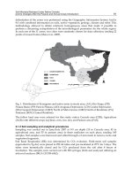
Summer
Fig. 7. Seasonal latent heat maps ET [W/m
2
] for the Serraia basin (TN, Italy).

Fig. 8. Example of evapotranspiration ET for the Serraia basin, Italy. Notice the elevation
effect (areas more elevated have less evaporation); the aspect effect (more evaporation in
southern slopes, left part of the image); the topographic convergence effect on water
availability (at the bottom of the valley).
397
Modelling Evapotranspiration and the Surface Energy Budget in Alpine Catchments
22 Will-be-set-by-IN-TECH
Differences in aspect :Continuous =N, Dot =S
Flussi
-200
-100
0
100
200
300
400
500
600
700
800
16/5/00 0.00 17/5/00 0.00 18/5/00 0.00 19/5/00 0.00 20/5/00 0.00
W/m
2
Rn 1 G 1 H 1 ET 1 dEdT 1 Rn G H ET
Fig. 9. Difference in energy balance between locations with the same properties but different
aspect. Dotted lines are for a south aspect location, while continuos lines are for a north
aspect location. It can be noticed how south aspect locations have larger R
n
and H, but
similar behavior for the other fluxes.

Flussi
-200
-100
0
100
200
300
400
500
600
700
800
16/5/00 0.00 17/5/00 0.00 18/5/00 0.00 19/5/00 0.00 20/5/00 0.00
W/m
2
Rn G H ET dE/dt
Rn G H ET dE/dt
Differences in saturation:Continuous sat=0.95, Dot=0.35
Fig. 10. Difference in energy balance between locations with the same properties but different
soil saturation. Dotted lines are for a dry location, while continuos lines are for wet location.
It can be noticed how wet locations have larger ET and lower H, but similar behavior for the
other fluxes. The time lag in R
n
is due to differences in aspect.
398
Evapotranspiration – Remote Sensing and Modeling
Modelling Evapotranspiration and the Surface Energy Budget in Alpine Catchments 23
(Albertson & Parlange, 1999). Moreover, horizontal differences in surface fluxes can start local
air circulations, which can affect temperature and wind surface values with a feedback effect.
How much such processes may affect the energy and water balance of the whole basin is easy

to quantify, but GEO
TO P
can be a powerful tool to explore these issues.
7. Conclusion
This chapter illustrates the components of the energy budget needed to model
evapotranspiration (ET) and provides an extended review of the fundamental equations and
parametrizations available in the hydrological and land surface models literature. In alpine
areas, ET spatial distribution is controlled by the complex interplay of topography, incoming
radiation and atmospheric processes, as well as soil moisture distribution, different land
covers and vegetation types. An application of the distributed hydrological model GEOtop
to a small basin is shown here, in order to bring out the problems arising when passing from
local one-dimensional scale to basin-scale ET models.
8. References
Albertson, J., Kustas, W. P. & Scanlon, T. M. (2001). Large-eddy simulation over
heterogeneous terrain with remotely sensed land surface conditions, Water Resour.
Res. 37: 1939–1953.
Albertson, J. & Parlange, M. B. (1999). Natural integration of scalar fluxes from complex
terrain, Adv. Water Resour. 23: 239–252.
Bartelt, P. & Lehning, M. (2002). A physical snowpack model for the swiss avalanche warning:
Part i: numerical model, Cold Regions Science and Technology 35(3): 123–145.
Bertola, P. & al. (2002). "studio integrato dell’eutrofizzazione del lago della serraia", Atti del
XXVIII Convegno di Idraulica e Costruzioni Idrauliche 3: 403–413.
Bertoldi, G., Kustas, W. P. & Albertson, J. D. (2008). Estimating spatial variability in
atmospheric properties over remotely sensed land-surface conditions, J. Appl. Met.
and Clim. 47(doi: 10.1175/2007JAMC1828.1): 2147–2165.
Bertoldi, G., Notarnicola, C., Leitinger, G., Endrizzi, S., ad S. Della Chiesa, M. Z. & Tappeiner,
U. (2010). Topographical and ecohydrological controls on land surface temperature
in an alpine catchment, Ecohydrology 3(doi:10.1002/eco.129): 189 – 204.
Bertoldi, G., Rigon, R. & Over, T. (2006). Impact of watershed geomorphic characteristics on
the energy and water budgets., Journal of Hydrometeorology, 7: 389–403.

Bertoldi, G., Tamanini, D., Endrizzi, S., Zanotti, F. & Rigon, R. (2005). GEOtop 0.875: the
programmer’s manual, Technical Report DICA-05-002, University of Trento E-Prints.
In preparation.
Best, M. J. (1998). A model to predict surface temperatures, Bound. Layer Meteorol.
88(2): 279–306.
Beven, K. J. & Freer, J. (2001). A dynamic TOPMODEL, Hydrol. Proc. 15: 1993–2011.
Beven, K. J. & Kirkby, M. J. (1979). A physically-based variable contributing area model of
basin hydrology, Hydrol. Sci. Bull. 24(1): 43–49.
Bonan, G. (1996). A land surface model for ecological, hydrological, and atmospheric studies:
technical description and user’s guide., Technical Note NCAR/TN-417+STR, NCAR,
Boulder, CO.
399
Modelling Evapotranspiration and the Surface Energy Budget in Alpine Catchments
24 Will-be-set-by-IN-TECH
Brooks, P. D. & Vivoni, E. R. (2008a). Mountain ecohydrology: quantifying the role
of vegetation in the water balance of montane catchments, Ecohydrol. 1(DOI:
10.1002/eco.27): 187 – 192.
Brooks, P. & Vivoni, E. R. (2008b). Mountain ecohydrology: quantifying the role of vegetation
in the water balance of montane catchments., Ecohydrology 1: 187–192.
Brutsaert, W. (1975). On a derivable formula for long-wave radiation from clear skies, Water
Resour. Res. 11(5): 742–744.
Brutsaert, W. (1982). Evaporation into the Atmosphere: Theory, Hystory and Applications, Kluver
Academic Publisher.
Businger, J. A., Wyngaard, J. C., Izumi, Y. & Bradley, E. F. (1971). Flux profile relationships in
the atmospheric surface layer, J. Atmospheric Sciences 28: 181–189.
Chow, F. K., Weigel, A. P., Street, R. L., Rotach, M. W. & Xue, M. (2006). High-resolution
large-eddy simulations of flow in a steep alpine valley. Part I: methodology,
verification, and sensitivity experiments, J. Appl. Met. and Clim. pp. 63–86.
Clapp, R. B. & Hornberger, G. M. (1978). Empirical equations for some hydraulic properties,
Water Resour. Res. 14: 601–605.

Cordano, E. & Rigon, R. (2008). A perturbative view on the subsurface
water pressure response at hillslope scale, Water Resour. Res.
44(W05407): doi:10.1029/2006WR005740.
Daamen, C. C. & Simmonds, L. P. (1997). Soil, water, energy and transpiration, a numerical
model of water and energy fluxes in soil profiles and sparse canopies, Technichal
report, University of Reading.
Dall’Amico, M. (2010). Coupled water and heat transfer in permafrost modeling, PhD thesis,
Institute of Civil and Environmental Engineering, Universita’ degli Studi di Trento,
Trento. Available from />Dall’Amico, M., Endrizzi, S., Gruber, S. & Rigon, R. (2011). A robust and energy-conserving
model of freezing variably-saturated soil, The Cryosphere 5(2): 469–484.
URL: />Deardorff, J. W. (1978). Efficient prediction of ground surface temperature and moisture with
inclusion of a layer of vegetation, J. Geophys. Res. 83(C4): 1889–1903.
Dickinson, R. E., Heanderson-Sellers, A., Kennedy, P. J. & Wilson, M. (1986). Biosphere
Atmosphere Transfer Scheme (BATS) for the NCAR Community Climate Model,
Technical Note NCAR/TN-275+STR, NCAR.
Dubayah, A., Dozier, J. & Davis, F. W. (1990). Topographic distribution of clear-sky radiation
over the Konza Prairie, Kansas, Water Resour. Res. 26(4): 679–690.
Endrizzi, S., Bertoldi, G., Neteler, M. & Rigon, R. (2006). Snow cover patterns and evolution at
basin scale: GEOtop model simulations and remote sensing observations, Proceedings
of the 63rd Eastern Snow Conference, Newark, Delaware USA, pp. 195–209.
Endrizzi, S. & Marsh, P. (2010). Observations and modeling of turbulent fluxes during melt
at the shrub-tundra transition zone 1: point scale variations, Hydrology Research
41(6): 471–490.
Erbs, D. G., Klein, S. A. & Duffie, J. A. (1982). Estimation of the diffuse radiation fraction for
hourly, daily and monthly average global radiation., Sol. Energy 28(4): 293–304.
Feddes, R., Kowalik, P. & Zaradny, H. (1978). Simulation of field water use and crop yield,
Simulation Monographs, PUDOC, Wageningen, p. 188pp.
400
Evapotranspiration – Remote Sensing and Modeling

Modelling Evapotranspiration and the Surface Energy Budget in Alpine Catchments

401
Garen, D. C. & Marks, D. (2005). Spatially distributed energy balance snowmelt modeling in
a mountainous river basin: estimation of meteorological inputs and verification of
model results, J. Hydrol. 315: 126–153.
Garratt, J. R. (1992). The Atmospheric Boundary Layer, Cambridge University Press.
Heimsath, M. A., Dietrich, W. E., Nishiizumi, K. & Finkel, R. (1997). The soil production
function and landscape equilibrium, Nature 388: 358–361.
Helbig, N., Lowe, H.&Lehning, M. (2009). Radiosity approach for the short wave surface
radiation balance in complex terrain., J.Atmos.Sci. 66(doi:10.1175/2009JAS2940.1):
2900–2912.
Iqbal, M. (1983). An Introduction to Solar Radiation, Academic Press.
Ivanov, V. Y., Vivoni, E. R., Bras, R. L. & Entekhabi, D. (2004). Catchment hydrologic
response with a fully distributed triangulated irregular network model, Water
Resour. Res. 40: doi:10.1029/2004WR003218.
Jarvis, P. & Morrison, J. (1981). The control of transpiration and photosynthesis by the
stomata., in P. Jarvis & T. Mansfield (eds), Stomatal Physiology, Cambridge Univ.
Press, UK, pp. 247–279.
Katul, G. G. & Parlange, M. B. (1992). A penman-brutsaert model for wet surface
evaporation, Water Resour. Res. 28(1): 121–126.
Kondratyev, K. Y. (1969). Radiation in the atmosphere, Academic Press, New York.
Kot, S. C. & Song, Y. (1998). An improvement of the Louis scheme for the surface layer in an
atmospheric modelling system, Bound. Layer Meteorol. 88(2): 239–254.
Kunstmann, H. & Stadler, C. (2005). High resolution distributed atmospheric-hydrological
modelling for alpine catchments, J. Hydrol. 314: 105–124.
Law, B. E., Cescatti, A. & Baldocchi, D. D. (1999). Leaf area distribution and radiative
transfer in open-canopy forests: Implications to mass and energy exchange., Tree
Physiol. 21: 287–298.
Louis, J. F. (1979). A parametric model of vertical eddy fluxes in the atmosphere, Bound.

Layer Meteorol. 17: 187–202.
Manabe, S. (1969). Climate and ocean circulation. i. the atmospheric circulation and the
hydrology of the earth’s surface., Monthly Weather Review 97: 739–774.
Mengelkamp, H.,Warrach, K. & Raschke, E. (1999). SEWAB - a parametrization of the
surface energy and water balance for atmospheric and hydrologic models,
Adv.Water Resour. 23: 165–175.
Monin, A. S. & Obukhov, A. M. (1954). Basic laws of turbulent mixing in the ground layer of
the atmosphere, Trans. Geophys. Inst. Akad. 151: 163–187.
Montaldo, N. & Albertson, J. (2001). On the use of the force-restore svat model formulation
for stratified soils, J. Hydromet. 2(6): 571–578.
Noilhan, J. & Planton, S. (1989). A simple parametriztion of land surface processes for
meteorological models, Mon. Wea. Rev 117: 536–585.
Paltrige, G. W. & Platt, C. M. R. (1976). Radiative Processes in Meteorology and Climatology
,
Else
vier.
Parlange, M. B., Eichinger,W. E. & Albertson, J. D. (1995). Regional scale evaporation and the
atmospheric boundary layer, Reviews of Geophysic 33(1): 99–124.
Philip, J. R. & Vries, D. A. D. (1957). Moisture movement in porous materials under
temperature gradients, Trans. Am. Geophys. Union 38(2): 222–232.
26 Will-be-set-by-IN-TECH
Prata, A. J. (1996). A new long-wave formula for estimating downward clear-sky
radiation at the surface., Quarterly Journal of the Royal Meteorological Society 122(doi:
10.1002/qj.49712253306): 1127–1151.
Richards, L. A. (1931). Capillary conduction of liquids in porous mediums, Physics 1: 318–333.
Rigon, R., Bertoldi, G. & Over, T. M. (2006). GEOtop: a distributed hydrological model with
coupled water and energy budgets, Journal of Hydrometeorology 7: 371–388.
Romano, N. & Palladino, M. (2002). Prediction of soil water retention using soil physical data
and terrain attributes, J. Hydrol. 265: 56–75.
Salvaterra, M. (2001). Applicazione di un modello di bilancio idrologico al bacino del Lago di Serraia

(TN), Tesi di diploma, Corso di diploma in Ingegneria per l’Ambiente e le Risorse.
Saravanapavan, T. & Salvucci, G. D. (2000). Analysis of rate-limiting processes in
soil evaporation with implications for soil resistance models, Adv. Water Resour.
23: 493–502.
Scanlon, T. M. & Albertson, J. D. (2003). Water availability and the spatial complexity of
co2, water, and energy fluxes over a heterogeneous sparse canopy, J. Hydromet.
4(5): 798–809.
Stull, R. B. (1988). An Introduction to Boundary Layer Meteorology, Kluwer Academic Publisher.
Van Genuchten, M. T. (1980). A closed-form equation for predicting the hydraulic conductivity
of unsaturated soils., Soil Sci. Soc. Am. J. 44: 892–898.
Warrach, K., Stieglitz, M., Mengelkamp, H. & Raschke, E. (2002). Advantages of
a topographically controlled runoff simulation in a SVAT model, J. Hydromet.
3: 131–148.
Wigmosta, M. S., Vail, L. & Lettenmaier, D. (1994). A Distributed Hydrology-Vegetation Model
for complex terrain, Water Resour. Res. 30(6): 1665–1679.
Wohlfahrt, G., Bahn, M., Newesely, C. H., Sapinsky, S., Tappeiner, U. & Cernusca, A. (2003).
Canopy structure versus physiology effects on net photosynthesis of mountain
grasslands differing in land use., Ecological modelling. 170: 407–426.
Wood, E. F. (1991). Land-surface-atmosphere interactions for climate modelling. observations,
models and analysis, Surv. in Geophys. 12: 1–3.
Zanotti, F., Endrizzi, S., Bertoldi, G. & Rigon, R. (2004). The geotop snow module, Hydrol. Proc.
18: 3667–3679. DOI:10.1002/hyp.5794.
402
Evapotranspiration – Remote Sensing and Modeling
18
Stomatal Conductance Modeling to
Estimate the Evapotranspiration of
Natural and Agricultural Ecosystems
Giacomo Gerosa
1

, Simone Mereu
2
, Angelo Finco
3
and Riccardo Marzuoli
1,4

1
Dipartimento Matematica e Fisica, Università Cattolica
del Sacro Cuore, via Musei 41, Brescia
2
Dipartimento di Economia e Sistemi Arborei, Università di Sassari,
3
Ecometrics s.r.l., Environmental Monitoring and Assessment,
via Musei 41, Brescia
4
Fondazione Lombardia per l’Ambiente, Piazza Diaz 7, Milano
Italy
1. Introduction
This chapter presents some of the available modelling techniques to predict stomatal
conductance at leaf and canopy level, the key driver of the transpiration component in the
evapotranspiration process of vegetated surfaces. The process-based models reported, are
able to predict fast variations of stomatal conductance and the related transpiration and
evapotranspiration rates, e.g. at hourly scale. This high–time resolution is essential for
applications which couple the transpiration process with carbon assimilation or air
pollutants uptake by plants.
2. Stomata as key drivers of plant’s transpiration
Evapotranspiration from vegetated areas, as suggested by the name, has two different
components: evaporation and transpiration. Evaporation refers to the exchange of water
from the liquid to the gaseous phase over living and non-living surfaces of an ecosystem,

while transpiration indicates the process of water vaporisation from leaf tissues, i.e. the
mesophyll cells of leaves. Both processes are driven by the available energy and the drying
potential of the surrounding air, but transpiration depends also on the capacity of plants to
replenish the leaf tissues with water coming from the roots through their hydraulic
conduction system, the xylem. This capacity depends directly on soil water availability (i.e.
soil water potential), which contributes to the onset of the water potential gradient within
the soil-plant-atmosphere continuum.
Moreover, since the cuticle -a waxy coating covering the leaf surface- is nearly impermeable
to water, the main part of leaf transpiration (about 95%) results from the diffusion of water
vapour through the stomata. Stomata are little pores in the leaf lamina which provide low-
resistance pathways to the diffusional movement of gases (CO
2
, H
2
O, air pollutants) from