Báo cáo hóa học: " Research Article Error Control in Distributed Node Self-Localization" ppt

Hindawi Publishing Corporation
EURASIP Journal on Advances in Signal Processing
Volume 2008, Article ID 162587, 13 pages
doi:10.1155/2008/162587
Research Article
Error Control in Distributed Node Self-Localization
Juan Liu and Ying Zhang
Palo Alto Research Center, 3333 Coyote Hill Road, Palo Alto, CA 94304, USA
Correspondence should be addressed to Juan Liu,
Received 31 August 2007; Accepted 7 December 2007
Recommended by Davide Dardari
Location information of nodes in an ad hoc sensor network is essential to many tasks such as routing, cooperative sensing, and
service delivery. Distributed node self-localization is lightweight and requires little communication overhead, but often suffers
from the adverse effects of error propagation. Unlike other localization papers which focus on designing elaborate localization
algorithms, this paper takes a different perspective, focusing on the error propagation problem, addressing questions such as where
localization error comes from and how it propagates from node to node. To prevent error from propagating and accumulating,
we develop an error-control mechanism based on characterization of node uncertainties and discrimination between neighboring
nodes. The error-control mechanism uses only local knowledge and is fully decentralized. Simulation results have shown that the
active selection strategy significantly mitigates the effect of error propagation for both range and directional sensors. It greatly
improves localization accuracy and robustness.
Copyright © 2008 J. Liu and Y. Zhang. This is an open access article distributed under the Creative Commons Attribution License,
which permits unrestricted use, distribution, and reproduction in any medium, provided the original work is properly cited.
1. INTRODUCTION
In ad hoc networks, location information is critical to many
tasks such as georouting, data centric storage, spatio-temp-
oral information dissemination, and collaborative signal
processing. When global positioning system (GPS) is not
available (e.g., for indoor applications) or not accurate and
reliable enough, it is important to develop local positioning
system (LPS). Recent years have seen intense research on this
topic [1]. One approach for LPS is to use fingerprinting that

requires extensive preparatory manual surveying and calibra-
tion [2–6] and is not reliable in terms of dynamic changes of
the environment. The other approach is for devices to self-
localize by collectively determining their positions relative to
each other using distance [7] or directional [8, 9] sensing in-
formation. Our research is focused on self-localization.
Node self-localization techniques can be classified into
two categories: centralized algorithms based on global op-
timization, and distributed algorithms using local informa-
tion with minimal communication. While the first cate-
gory methods are powerful and produce good results, they
require substantial communication and computation, and
hence may not be amendable to in-network computation of
location information on resource-constrained networks such
as sensor networks. In this paper, we focus on the second cat-
egory, distributed node self-localization. Various distributed
node localization techniques have been proposed in the sen-
sor network literature [10, 11]. The basic idea is to decom-
pose a global joint estimation problem into smaller subprob-
lems, which only involve local information and computa-
tion. Then localization iterates over the subproblems [12–
16]. This approach greatly reduces computational complex-
ity and communication overhead.
However, one problem with distributed localization is
thatitoftensuffers from the adverse effects of error propa-
gation and accumulation. As a node being localized and be-
coming new anchor for other free nodes, the estimation error
in the first node’s location can propagate to other nodes and
potentially get amplified. The error could accumulate over
localization iterations, and this may lead to unbounded error

in localization for large networks. The effect of error propa-
gation may also occur in global methods such as MDS [17]
or SDP [18, 19], but is less prominent, due to the fact that
global constraints tend to balance against each other.
Although the error characteristics of localization have
been studied in literature [20, 21], the problem of error con-
trol has not received adequate attention. Our early work [22]
is the first paper presenting the idea of using a node registry
to formally characterize error in iterations and choose neigh-
bors selectively in localization to filter out outlier estimates
2 EURASIP Journal on Advances in Signal Processing
(bad seeds) that may otherwise contaminate the entire net-
work. In this paper, we extend the early work and present a
more general error-control mechanism, applicable to a va-
riety of sensing modalities, such as range sensors (time-of-
arrival (TOA) or received-signal-strength (RSS)) and direc-
tional sensors (camera, microphone array, etc). The error
control consists of three components: (1) error characteri-
zation to document node location with uncertainty; (2) a
neighbor selection step to screen out unreliable neighbors—
it is preferable to only use nodes with low uncertainty to lo-
calize others; this prevents error propagating to other nodes
and contaminating the entire network; (3) an update criterion
that rejects a location estimate if its uncertainty is too high;
this cuts the link of error accumulation. This error-control
mechanism is lightweight, and only uses local knowledge.
Although we will be presenting localization algorithms
in later sections, for example, the iterative least-squares (ILS)
algorithm for range-based localization and the geometric ray
intersection and mirror reflection algorithms for direction-

based localization, we would like to point out that the focus
of this paper is not on any particular localization algorithm,
but rather on controlling error in order to mitigate the effect
of error propagation. It is a simple fact that all localization
schemes are imperfect and result in some error. Most work
in the localization literature focuses on elaborate design of
localization algorithms and fine-tuning to produce small lo-
calization error. In this paper, we take a different perspec-
tive by addressing questions such as where localization error
comes from, how it can propagate from node to node, and
how to control it. We explain in details how the error-control
mechanism is devised to manage information with various
degree of uncertainty. Our method has been tested in sim-
ulations. Results have shown that the error-control mecha-
nism is powerful in mitigating the effect of error propaga-
tion. It significantly improves localization performance and
speeds up convergence in iterations. For range-based local-
ization, despite the fact that the underlying localization (ILS)
is very simple, it achieves performance comparable to and
in many cases better than that of more global methods such
as MDS-MAP [17] or SDP [19]. Similar improvements have
been observed in our early experiments on a small network of
Mica2 motes with ultrasound time-of-arrival ranging [22].
For directional-based localization, we show that the error-
control method outperforms the basic localization mecha-
nism [8], reducing localization error by a factor of 3-4. Ex-
periments on a real platform using the Ubisense real-time
location system [23] will be conducted in the near future.
This paper is organized as follows. Section 2 presents the
overview of the distributed node self-localization. Section 3

describes the error-control mechanism. Sections 4 and 5 ap-
ply this mechanism to range-based and angle-based node lo-
calization, respectively. Section 6 concludes the paper.
2. DISTRIBUTED LOCALIZATION: AN OVERVIEW
Most localization approaches assume that a small number of
anchor nodes know their location a priori and then progres-
sively localize other nodes with respect to the anchors. An-
chorless localization is also feasible for some algorithms, such
as building relative maps using MDS-MAP [17] or forming
rigid structures between nodes as described in [24]. It is pos-
sible to develop error control for anchorless localization, but
this requires a more elaborate mechanism which remains our
future research. In this paper, we assume the existence of a
small set of anchor nodes.
In general, localization is to derive unknown node lo-
cations
{x
t
}
t=1, ,N
based on a set of sensor measurements
{z
t,i
} and anchor node locations. Each measurement pro-
vides a constraint on the relative position between a pair
of sensors. In this paper, we consider the two most com-
monly used sensor types: range sensors and directional sen-
sors. Both types have a large variety of commercially avail-
able products. A range sensor provides distance information
between nodes, typically derived from sensing of physical

signals such as acoustic, ultrasonic, or RF transmitted from
one node to another. Distance can be derived from time-of-
arrival (TOA) measuring time of flight between the sender
and the receiver, or via received signal strength (RSS) follow-
ing a model of signal attenuation. A directional sensor mea-
sures the relative direction from one node to another, that is,
(x
i
− x
t
)/x
i
− x
t
. There are ample examples of directional
sensors: cameras [25], microphone arrays with beamforming
capability, UWB positioning hardware such as the Ubisense
product []. Without loss of general-
ity, we consider localizations in a 2D plane. Most of the tech-
nical points illustrated in 2D can readily be extended to 3D.
Distributed node localization is iterative in nature. We
use multilateration-type localization [12] as a vehicle for il-
lustration. Initially, only anchor nodes are aware of their lo-
cations. A free node is localized by incorporating sensor mea-
surements from anchors in its local neighborhood N . In the
case of range sensors, a free node can be localized if it can
sense at least 3 nodes with known locations. The newly local-
ized free nodes are then used as “pseudoanchors” to localize
other neighboring free nodes. Here neighbors are not topo-
logical neighbors in a communication network, but rather

in a sensing network graph (SNG) defined as follows: ver-
texes are sensor nodes, and edges represent distance or an-
gle constraints between pairs of nodes. Any pair of nodes
that can reliably sense each other’s signal (hence form sen-
sor measurement z
t,i
)arecalledmutualimmediate neighbors
in SNG. We assume that neighbors in SNG can communi-
cate with each other, either directly or via some intermediate
node; in most cases, communication ranges are larger than
sensing ranges. Each iteration progressively pushes location
information over edges of SNG, for example, from anchors
to nearby free nodes, and from pseudoanchors to their neigh-
bors. The iteration may terminate if node locations no longer
change or if a computation allowance has been exhausted.
Algorithm 1 shows the iterative procedure. Technically, one
iteration means one complete sweep in the do-while loop.
We assume that the nodes are updating their locations in
a globally synchronous fashion, that is, each free node up-
dates their location based on the information of its neighbors
from the previous iteration. The updates can be done simul-
taneously across nodes. There are various research work on
packet scheduling to avoid collision, for instance, using pre-
assigned time-slot in TDMA. In this paper, we do not discuss
J. Liu and Y. Zhang 3
ITERATIVE LOCALIZATION
Each node i holds x,where
x
i
is the node location (or estimate);

x
i
= null if location is unknown
Free node to be localized is denoted by t
Each edge corresponds to a measurement z
t,i
;
do
{
for each free node t
examine local neighborhood N ;
find all neighbors in N with known location
compute location estimate
x
t
;
} while termination condition is not met.
Algorithm 1: Iterations in distributed multilateration.
the packet scheduling problem. Note that the procedure in
Algorithm 1 does not rely on a collision-free communication
assumption. If a free node does not receive enough informa-
tion from its neighbors due to collision, it just skip the state
of computing a location estimate and remains unknown.
3. ERROR CONTROL IN ITERATIVE LOCALIZATION
Distributed localization such as the procedure illustrated in
Algorithm 1 often suffers from error propagation. Estimated
node locations are not perfect. Their uncertainty may further
influence neighboring nodes. Over iterations, the error may
propagate to the entire network. Essentially, error propaga-
tion is caused by the strategy of using the estimated node

locations as pseudoanchors to localize other nodes. While
this strategy greatly reduces the amount of communication
and computation required and is more scalable, it also intro-
duces potential degradation in localization quality. The opti-
mization strategy is analogous to a coordinate descent algo-
rithm, which, at any step, fixes all but one coordinate (node
location in this case), finds the best solution along the flex-
ible axis, and iterates over all axes. Just as a coordinate de-
scent algorithm may have slow convergence and get stuck at
ridges or local optima, this node localization strategy suffers
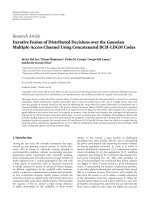
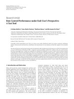
from similar problems. Figure 1 shows a typical run where
localization gets stuck. Moreover, the strategy may be slow
to converge which means high communication and compu-
tation overhead. Even global optimization schemes are not
completely immune to error propagation. For example, the
relaxation method of [19] introduces the possibility of error
propagation. The existence of error propagation is inherently
a by-product of the optimization strategies.
Various heuristics are proposed to mitigate the effect of
error propagation. For example, [26] weights multilateration
results with estimated relative confidence, and [7] discounts
the effect of measurements from distant sensors based on the
intuition that they are less reliable and may amplify noise.
Recent work on cluster-based localization [24] selects spa-
tially spread nodes to form quadrilaterals to minimize local-
ization error. In this paper, rather than using heuristics, we
seek to provide a formal analysis of localization error.
1009080706050403020100
100
90

80
70
60
50
40
30
20
10
0
Figure 1: Localization gets stuck at a local optimum. Estimated
node locations are marked with diamonds, true locations are plot-
ted as dots, and solid lines show the displacement between the esti-
mated locations and the ground truth (i.e., each line is the estima-
tion error of a node). Anchors are marked with circles.
The basic idea of error control is simple: when a node
is localized with respect to its neighbors, not all neighbors
are equal. Certain neighbors may have more reliable location
information than others. It is hence preferable to use only
reliable neighbors to avoid error propagation. Based on this
intuition, we propose an error-control method consisting of
three components as follows.
(1) Error characterization. Each time we compute a loca-
tion estimate, we perform the companion step of char-
acterizing the uncertainty in the estimate. Each node
maintains a registry that contains the tuple (location
estimate, location error). It is useful in the next round
for neighbor selection (see Algorithm 2).
(2) Neighbor selection. This step differentiates neighbors
based on uncertainty in their respective node reg-
istries. Nodes with high uncertainty are excluded from

the neighborhood and not used to localize others. This
prevents errors from propagating.
(3) Update criterion. At each iteration, if a new estimated
location has error larger than the current error or a
predefined threshold, the new estimate is discarded.
This conditional update criterion prevents error from
generating.
Algorithm 2 shows the same iterative localization procedure
as in Algorithm 1 but with error control. The error-control
steps are marked in italic fonts. Note that for this error-
control mechanism to work, the free node would have to
know not only the location of its neighbors, but also their
respective uncertainty e
v
. From a practical implementation
point of view, the uncertainty information can be piggy-
backed on the same packet when the location information
4 EURASIP Journal on Advances in Signal Processing
ITERATIVE LOCALIZATION WITH ERROR CONTROL
Each node i holds the tuple (x, e
v
)
i
,where
x
i
is the node location (or estimate) of neighbor i;
e
v
i

(vertex error) is the uncertainty in x
i
.
The free node to be localized is denoted as t
Each edge j corresponds to a tuple (z, e
e
)
t,i
,where
z
t,i
is the sensor measurement regarding node t and neighbor i;
e
e
t,i
(edge error) is the uncertainty in z
t,i
do {
for each free node t
examine local neighborhood N ;
select neighbors based on vertex and edge errors
{e
v
} and {e
e
}
compute location estimate x
t
;
estimate error

e
t
;
decide whether to update t’s registry with the new tuple (
x
t
, e
t
).
}while termination condition is not met.
Algorithm 2: Distributed localization with error control. The error-control steps are shown in italic fonts.
is sent. The edge error is known from sensing characteristics
and does not require additional communication.
In this section, we address the design principles of error
control, and defer the detailed implementation to Sections 4
and 5.
3.1. Error characterization
The basic problem of localization is, for any free node t,given
its neighbor locations
{x
i
}
i∈N
and the corresponding sensor
measurements
{z
t,i
}
i∈N
,howtoobtainanestimate

x
t
= f

x
i

,

z
t,i

. (1)
Localization error of a nonanchor node t comes from two
sources.
(1) Uncertainty in each neighbor location x
i
. A neighbor
may have imperfect information regarding its location,
especially nonanchor nodes. We call this error “vertex
error” (because a neighbor is a vertex in the SNG) and
use the shorthand notation e
v
.
(2) Uncertainty in each sensor measurement z
t,i
.Wecall
this “edge error” and use the notation e
e
.

The error
e
t
in the location estimate x
t
is a function of both
vertex and edge errors:
e
t
= g


e
v
i

i∈N
,

e
e
(t,i)

i∈N

. (2)
In this paper, we seek to find the proper form of g(
·, ·)to
characterize error. In the iterative localization process, the er-
ror characterization is recursive: the node derives error char-

acteristicsbasedonvertexandedgeerrorsfromitslocalre-
gion. In the next round, this node is used to localize others,
hence its error
e
t
becomes the vertex error e
v
for the neigh-
boring nodes.
Despite the simple formulation, error characterization
is difficult. Ideally, one would like to express uncertainty as
probability distribution, for example, e
v
i
= p(x
i
), and derive
the exact form of
e
t
. But anyone with even superficial knowl-
edge on statistics will recognize the difficulty: it is extremely
hard to derive a distribution of f (a, b, c) from the distribu-
tion of its individual variables a, b,andc.Thefunction f
could be complicated, and the variable may be dependent,
in which case we need the joint distribution p(a, b,c). As
localization progresses, the error characterization problem
quickly becomes intractable. To overcome the difficulty, we
make several grossly simplifying assumptions. First, we as-
sume all variables are Gaussian, in which case the uncertainty

can be characterized by a variance (for scalar) or a covari-
ance matrix (for vectors). This reduces the form of e
v
and e
e
down from a probability distribution to only a few numbers.
Secondly, we assume that the function f can be linearized
with only mild degradation. This assumption is necessary
because only when f is linear will the result
x
t
(1)remain
Gaussian. Thirdly, we assume that variables in (1) are inde-
pendent, hence the covariance e
t
will be the sum of the con-
tribution from each variable x
i
’s and z
t,i
’s. These simplifying
assumptions enable us to carry forward error characteriza-
tion with the progression of localization, and to differentiate
node qualitatively. We recognize that these assumptions are
sometimes inaccurate. In contrast, the exact quantitative dif-
ferentiation is out of reach. Furthermore it may not be neces-
sary since our goal is to rank neighbors and select a subset of
good ones, hence any qualitative measure producing roughly
the same order and the same subset should suffice.
In our scheme, each node t has a registry containing the

tuple (x
t
, e
v
t
). We will illustrate in details how x
t
and e
v
t
are
computed in localization using range sensors and directional
sensors in later sections (Sections 4 and 5,resp.).Wenote
that any location estimation step is followed by the compan-
ion step of computing the uncertainty of the location esti-
mate. This effectively doubles the computation complexity
in each iteration. Is it worthwhile? We will be addressing
this question using simulation experiments. We would also
J. Liu and Y. Zhang 5
like to point out that although error characterization is de-
signed to discriminate neighbors in localization iterations,
it can also be used in follow-up tasks after localization. For
example, tasks such as in-network signal processing need to
know node locations, but the performance may be further
enhanced if it also knows the rough accuracy of node loca-
tions. It can optimize with respect to this additional infor-
mation, even when such information is qualitative.
3.2. Neighbor selection
Neighbor selection has been proposed in several papers such
as [20, 21]todifferentiate neighbors based on heuristics

about the noise-amplifying effect of node geometry, or based
on estimation bounds such as Cramer-Rao lower bound
(CRLB). In this paper, we use formal error characterization
(2) to prepare the ground for neighbor selection. As we will
see in the later sections, geometry-like heuristics are often
special cases that can be easily derived from our error char-
acterization step. We do not use CRLB because it is often too
loose. In our method, we select neighbors based on their ver-
tex error and edge error. Vertex error is recorded in the node
registry. Neighboring nodes can be sorted based on their
respective registries. Edge error is the uncertainty in pair-
wise sensor measurements. This can be derived from sensing
physics.
3.3. Update criterion
Even with “high-quality” neighbors and good sensor mea-
surements with mild noise perturbation, the estimate could
still be arbitrarily bad if the neighbors happen to be in some
pathological configuration. For example, as we will see in
Section 4, collinearity in neighbor positions greatly amplifies
measurement noise and result in bad estimate. To address
this problem, we propose an update criterion to reject bad
estimates based on their quality. A few metrics can be used
here: (1) the uncertainty
e
v
t
:rejectifitistoobig;and(2)data
fitting error: reject if the estimate does not agree with sensor
observation data.
4. ERROR CONTROL IN LOCALIZATION USING

RANGE SENSORS
A range sensor measures the distance from itself to another
node, that is,
z
i
=


x − x
i


. (3)
Most localization schemes using range sensors are based
on multilateration, using distance constraints to form rigid
structures. If anchor density is low, we use an optional initial-
ization stage. During the initialization, anchor nodes broad-
cast their location information. Each free node computes a
shortest path in SNG to each of the nearby anchors, and use
the path length as an approximation to the Euclidean dis-
tance. The shortest path can be computed locally and effi-
ciently using Dijkstra’s algorithm. Note that it is sufficient for
a free node with shortest paths to 3
∼5 anchors to obtain an
initial location estimate. In this section, we first describe a
simple least-squares (LS) algorithm for location estimation,
then proceed to discuss the corresponding error characteri-
zation and error-control method.
4.1. Least-squares multilateration
Ignoring the measurement (edge) and neighbor location

(vertex) errors for the moment, we square both sides of (3)
and obtain
x
2
+


x
i


2
−2x
T
i
x = z
2
i
, i = 0, 1, (4)
From
|N | such quadratic constraints, we can derive n =
(|N |−1) linear constraints by subtracting the i = 0con-
straint from the rest as follows:
−2

x
i
−x
0


T
x =

z
2
i
−z
2
0

−



x
i


2
−


x
0


2

. (5)
The (i

= 0)th sensor is used as the “reference.” Letting a
i
=
−
2(x
i
−x
0
)andb
i
= (z
2
i
−z
2
0
) −(x
i

2
−x
0

2
), we simplify
the above as
a
T
i
x = b

i
. (6)
Here, a
i
is a 2 ×1vector,andb
i
is a single scalar.
Thus,wehaveobtainedn linear constraints, expressed in
matrix form
Ax
= b,(7)
where A
= (a
1
, a
2
, , a
n
)
T
and b = (b
1
, b
2
, , b
n
)
T
.The
least-squares solution to the linear system (7)is

x
t
= A
†
b,
where A
†
is the pseudoinverse of A, that is, A
†
= (A
T
A)
−1
A
T
.
In later text, we use the shorthand notation I
A
= (A
T
A)
−1
when necessary. This linearization formulation is commonly
used in localization; see [22, 26], for examples. The computa-
tion is lightweight, since A is only of size n
×2, with n typically
being small, and b is of size n
×1.
4.2. Error characterization and control
Intheformulationin(7), b captures the information about

sensor measurements, and A encodes the geometric infor-
mation about the sensor configuration. The accuracy of lo-
calization is thus influenced by these two factors. First, the
error in the measurement z’s (i.e., edge errors) will result in
some uncertainty in b. In particular, assume no vertex errors,
that is, A is certain, the error due to b can be characterized as
follows:
Cov

e
Δb

= Cov

A
†
Δb

= A
†
·Cov(Δb)·

A
†

T
.
(8)
A pathological case is that nodes are collinear. In this case,
A is singular, so is the pseudoinverse A

†
. With a large con-
dition number, A
†
greatly amplifies any slight perturbation
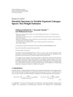
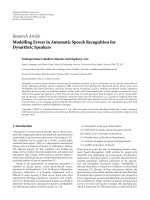
in b (i.e., measurement noise). This is the case shown in
Figure 2(a). The estimate, marked as a star, has a covari-
ance which is a long ellipsoid. In contrast, Figure 2(b) shows
a location estimation example where the neighbors are well
6 EURASIP Journal on Advances in Signal Processing
6543210
4.5
4
3.5
3
2.5
2
1.5
1
0.5
0
A
= (1, 1)
Estimated location
T
= (3, 2)
C
= (5, 1)
B
= (4, 0.5)

(a)
6543210
4.5
4
3.5
3
2.5
2
1.5
1
0.5
0
A
= (1, 1)
Estimated location
T
= (3, 2)
C
= (5, 1)
B
= (4, 4.5)
(b)
Figure 2: Estimation error for different neighbor geometry: (a) three almost collinear neighbors and (b) three neighbors forming a well-
spaced triangle. The estimate covariance is plotted as an ellipsoid.
spaced. In this case, A is well-conditioned, and the result es-
timation error is small.
Secondly, we consider the noise in neighbor locations
(vertex error). Note that we can reorganize elements in the
A matrix into a long vector a
= (a

11
, a
21
, , a
n1
, a
12
, a
22
,
, a
n2
)
T
, where the element a
ij
=−2(x
ij
− x
0,j
)fori =
1, , n and j = 1, 2 (n is the number of equations in (6)).
If the error statistics of x
i
’s are known, we can estimate the
statistics of Δa
ij
as well. Let matrix
B
Δ

=

b
1
b
2
··· b
n
00··· 0
00
··· 0 b
1
b
2
··· b
n

. (9)
It is easy to verify that A
T
b = Ba. Using this notation, the
original estimate x
t
= I
A
A
T
b can be written as x
t
= I

A
Ba.
Theerrorduetoa is
Cov

e
Δa

=
Cov

I
A
BΔa

=
I
A
BCov(Δa)B
T
I
A
T
.
(10)
The total error is the summation of the two terms listed
above. The overall analysis provides a way of evaluating (2)
from edge and vertex errors. Note that the computation of
error only involves multiplication of small matrices: A is of
size n

× 2, B is of size 2 × 2n, I
A
is of size 2 × 2, and the co-
variances Cov(Δa)andCov(Δb) are of size 2n
×2n and n×n,
respectively. No matrix inversion is involved.
With closed-form easy-to-evaluate error characteriza-
tion, error control becomes simple. The neighbor selection
step determines among the neighbors with known locations
whose measurement to use and whose to discard. We use a
simple heuristic. For any node i
∈ N (t), we sum up the ver-
tex error e
v
and the edge error e
e
for the edge between t and
i, that is, we compute a total score
e
total
(i) = e
v
i
+ e
e
(i,t)
. (11)
The nodes with lower sum are considered preferable. The
summation form of total error (11)ismerelyheuristic,but
makes intuitive sense: for any given node i,ifitisusedtolo-

calize others, its location error e
v
i
will add uncertainty to the
localized result
x
t
; furthermore, the measurement error e
e
(i,t)
will cause x
t
to drift around by roughly the same amount.
This is not exact though, because the final localization result
depends not only on node i, but on the geometry of all se-
lected neighbors. The exact error should be evaluated with
all neighbor combinations (2
|N |
combinations altogether).
Note that the goal of neighbor selection is not to find the
optimal combination of nodes, but rather to filter out out-
lier nodes with bad quality. Hence, we retreat to this simple
heuristics which has linear complexity o(
|N |).
In our implementation, the node with the lowest sum is
used as x
0
. The neighbor selection is done by ranking the
e
total

(i)’s in an ascending order, picking the first three nodes,
and setting a threshold that is 3σ above the third lowest e
total
value, where σ is the standard deviation of edge errors. Nodes
with the error sum below the threshold are selected. The
nodes that are 3σ above are considered outliers, and excluded
from the neighborhood. The 3σ threshold value is empirical,
which seems to work well in practice. The update criterion
examines the new estimate (
x
t
, e
t
) tuple, and rejects it if the
error
e
t
is larger than a predefined threshold.
4.3. Simulation experiment
The localization algorithm described above has been vali-
dated in simulations. A network is simulated in a 100 m
×
100 m field, with 160 nodes placed randomly according to
a uniform distribution. Each node has a sensing range of
20 m, which is 1/5 of the total field width. Anchor nodes are
randomly chosen. The standard deviation of anchor nodes
is 0.5 m in horizontal and vertical directions. Distance mea-
surements are simulated with Gaussian noise with zero mean
J. Liu and Y. Zhang 7
20181614121086420

No error control: 26 good runs
With error control: 30 good runs
0
5
10
15
20
25
30
35
40
45
Random layout, 10% anchors
(a)
20181614121086420
No error control: 29 good runs
With error control: 30 good runs
0
5
10
15
20
25
30
35
40
45
Random layout, 20% anchors
(b)
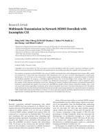
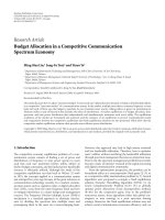
Figure 3: Localization accuracy for random network layout with (a) top panel: 10%, and (b) bottom panel: 20% randomly placed anchor

nodes. The horizontal axis is the number of iterations; the vertical axis is the average distance between location estimates and ground truth,
measured in meters.
and a variance of 1.5 m
2
. Since it is simulation, and the
ground truth is known, we use the location error ζ
x
=

t
|x
t
−x
t
|/N measuring the average deviation from ground
truthastheperformancemetric.
To study the effect of error control, we compare localiza-
tion performance with and without error control. The short-
est path initialization is not used in this experiment because
the anchor percentage is relatively high. The scheme with
error control actively selects from its neighborhood which
measurements to use and which to reject, using the error es-
timation described in Section 4.2. For each scheme, 30 in-
dependent runs are simulated in a network of TOA sensors
with 10% and 20% anchor nodes, respectively. We consider a
run “lost” if the localization scheme produces a larger error
than that of randomly selecting a point in the network layout
as the estimate; otherwise, we consider it a good run. With
error control, all 30 runs are good. In contrast, the scheme
without error control loses a few runs: 4 lost runs with 10%

anchor nodes and 1 lost run with 20% anchors.
Figure 3(a) reports the localization accuracy (with 10%
anchor nodes) at the beginning of each iteration, with ac-
curacy measured as location errors. The accuracy results are
plotted as circles and crosses, for localization with and with-
out error control, respectively. The first few iterations pro-
duce large localization error; this is because only a fraction of
the nodes is localized. After 4-5 iterations, almost all nodes
are localized, and after that the nodes iterate to refine their
location estimate. The figure clearly indicates that the er-
ror control strategy improves localization significantly. In
particular, error control speeds up localization. Figure 3(a)
shows that seven iterations in the scheme without error con-
trol produces a localization accuracy of about 11 m. With
error control, the localization accuracy improves to about
6 m. Furthermore, to achieve a given localization accuracy,
the scheme with error control needs far fewer iterations. For
example, in the same setting, error control takes about 6–8 it-
erations to stabilize. To achieve the same accuracy, more than
20 iterations are needed in the scheme without error control.
From the communication perspective, although error con-
trol requires the communication of error registry, it pays to
do so, since overall, much fewer rounds of communication
are needed.
The advantage of error control is most prominent when
the percentage of anchor nodes is low. As the percentage
increases, the improvement diminishes (Figure 3(b)). Intu-
itively, when the percentage is low, the effect of error prop-
agation is significant, and hence the benefit of error control.
With error control, each iteration takes more computation,

since the error registry need to be updated. We have simu-
lated our localization algorithm using MATLAB on a 1.8 GHz
Pentium II personal computer. In the baseline scheme, each
node takes about 1.2 milliseconds per iteration, and the er-
ror control scheme takes about 2.5 milliseconds. This rough
comparison shows that the amount of computation doubles
in each iteration. However, as we have shown in Figure 3, the
error control method takes less iterations to converge to a
given accuracy level and reduces lost track possibilities. So if
the accuracy requirement is high, the error control method
is recommended.
4.3.1. Comparison with global localization algorithms
There have been a number of other localization algorithms
proposed in the literature. Here, we refer to our scheme as the
8 EURASIP Journal on Advances in Signal Processing
Table 1: Instances of best localization results over 100 randomly
generated test data for networks with a large number of anchors.
Bold entries highlight the best performance for each case.
Anchor percentage MDS SDP ILSnspa ILS SPA
10% 39 0 20 42 0
20% 0 6 35 64 0
incremental least-squares- (ILS-) based method. We com-
pare ILS with the following methods:
(1) ILS: error controlled ILS with shortest path approxi-
mation in initialization;
(2) ILSnspa: error controlled ILS without shortest path ap-
proximation;
(3) MDS-MAP: localization based on multiscaling using
connectivity data [17]. It is very robust to noise and
low connectivity;

(4) SDP: localization based on semidefinite programming
[19], working well for anisotropic networks;
(5) SPA: localization using shortest-path length between
node pairs [27]. This is equivalent to the initialization
step of ILS without further iterations.
Among the methods, MDS-MAP and SDP are global in na-
ture, although heuristics have been used to distribute com-
putation. SPA is very simple and easy to implement in dis-
tributed networks and used as a baseline comparison.
To compare performance, we generate 100 random in-
stances of sensor field layout and run all the algorithms
for each instance. The first performance metric is error his-
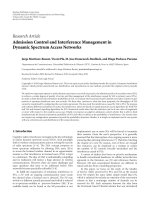
togram, shown in Figures 4(a) and 4(b) for each method
for 10% and 20% anchor nodes, respectively. Here, the his-
togram is drawn in the form of vertically stacked bars, each
bar indicates how many instances produce an average node
localization error ζ
x
in a certain range, for example, smaller
than 1.5, between 1.5 and 2.5, and so on. We favor method
with long bar for error < 1.5 (estimates being accurate) and
with short bar or no bar for large errors (estimates being ro-
bust). From this figure, we see that ILS performs well, com-
parable to MDP, better than SDP and SPA.
The second performance metric is best case performance,
which indicates the number of instances that an algorithm
produces the best results. If two algorithms produce the same
best result (within 0.01 accuracy), both will be counted.
Ta ble 1 shows the number of the best results over 100 in-
stances for 10% and 20% anchors, respectively. Again, we see

that ILS produces most instances of best result, outperform-
ing MDS and SDP global methods. This is amazing but not
entirely surprising, given that we have carefully avoided error
propagation and accumulation.
Our earlier work [22] has experimented with localization
using an extremely low anchor density, where the whole net-
work consists of only three anchors. This is the minimal re-
quirement for range-based localization. Similar performance
has been observed. In this setting, ILS performs much better
than MDS or SDP. Interested readers may refer to [22]for
more details.
5. ERROR CONTROL IN LOCALIZATION USING
DIRECTIONAL SENSORS
A directional sensor in a 2D plane has 3 degrees of freedom:
x-location, y-location, and a reference angle θ. Localization
attempts to estimate these parameters if they are unknown.
In a 3D space, the parameter set becomes (x-, y-, z-locations,
yaw, pitch, roll). In this paper, we focus on the 2D case for
simplicity. In this section, we first describe the basic localiza-
tion algorithm and then present the error control method.
5.1. Basic localization algorithm
Directional sensors are inherently more complicated than
range sensors and often more expensive in practice. To lo-
calize a set of directional sensors, we use the assistance of
objects, which can be sensed by multiple sensors simulta-
neously. For example, a directional sensor can be a cam-
era, and objects can be points in the field of view, especially
points with easy-to-detect structural features such as cor-
ners. From sensor observations (e.g., images), one can ex-
tract constraints regarding the relative position between sen-

sors and objects, and estimate unknown parameters in the
world coordinate. Another example of directional sensor is
radar, which uses beamforming technique to estimate the di-
rection of signal with respect to its reference angle. Objects
in this case can be airplanes.
The localization problem is formulated as follows. The
network consists of sensors S
={(x
i
, θ
i
)} and a number of
objects O
={x
o
}. To start with, we assume that only a few
sensors (anchors) know their parameters and no object pa-
rameters are known a priori. The goal of estimation is to es-
timate all S and O. For localization, we use an iterative ap-
proach that is similar to multilateration: from anchor sen-
sors, we estimate the location of neighboring objects; these
objects are then used to estimate other unknown sensors; and
so on. The algorithm alternates between using sensors to lo-
calize objects and using objects to estimate sensors, until the
localization converges or some termination criterion is met.
5.1.1. Localizing an object using several known sensors
This step is easy. Let x
i
and θ
i

be the location and orientation
of the sensor, respectively, and let α
i
be the angle of the object
from the sensor reference. Each measurement defines a ray
originated from the sensor:

−
sin

θ
i
+ α
i

cos

θ
i
+ α
i

·

x − x
i

=
0. (12)
Given that the object can be seen by a set of sensors, the ob-

ject location can be obtained by ray intersection, that is, by
solving a linear system Ax
= b,whereA = (a
1
, a
2
, , a
n
)
T
and b = (b
1
, b
2
, , b
n
)
T
,inwhicha
T
i
= (−sin(θ
i
+ α
i
),
cos(θ
i
+ α
i

)) and b
i
= a
T
i
x
i
.
5.1.2. Estimating a sensor using several objects with
known location
For this task, localization based on circle intersection has
been proposed, for instance, in [8, 9]. The basic idea is as
J. Liu and Y. Zhang 9
SPAILSnspa ILSSDPMDS
e<1.5
1.5 <e<2.5
2.5 <e<3.5
3.5 <e<4.5
e>4.5
0
10
20
30
40
50
60
70
80
90
100

Number of instances in each error range
(a)
SPAILSnspa ILSSDPMDS
e<1.5
1.5 <e<2.5
2.5 <e<3.5
3.5 <e<4.5
e>4.5
0
10
20
30
40
50
60
70
80
90
100
Number of instances in each error range
(b)
Figure 4: Error histograms: (a) 10% anchors and (b) 20% anchors.
follows: eliminating θ by taking the angle difference β
i,j
=
α
i
−α
j
, this produces the angle between the two rays from the

sensor to objects i and j. All possible locations of the sensor
form an arc, uniquely defined by the chord between object
i and object j and the inscribed angle β
i,j
. For example, in
Figure 5, it is easy to verify that the central angle ∠AO
AB
B is
2π
−2β
AB
,whereβ
AB
is the inscribed angle ∠ASB. We use the
notation
→
n
AB
to denote the unit vector orthogonal to x
B
−x
A
,
and derive the center position as
x
O
AB
=
x
A

+ x
B
2
+


x
A
−x
B


2tanβ
AB
·
−→
n
AB
.
(13)
The first term is the midpoint between A and B. The sec-
ond term travels along the radial direction
→
n
AB
by length
x
A
− x
B

/(2 tan β
AB
) to get to the center. Likewise, one can
also obtain the radius as
x
A
−x
B
/(2|sin β
AB
|).
The location of the sensor can be estimated by inter-
secting multiple arcs. Once the sensor location is known,
the reference angle can be estimated trivially. In this paper,
we use an equivalent method but with a slightly different
form, shown in Figure 5. Rather than intersecting two circles,
which is a nonlinear operation, we find sensor location S by
mirroring A with respect to the line linking the two centers
O
AB
and O
AC
. Mathematically,
x
S
= x
A
−2



x
A
−x
O
AB

T
·
→
n

→
n
, (14)
where
→
n
is the unit vector orthogonal to the line from O
AB
to
O
AC
. The second term in (14) is twice the projection of the
A
S
B
O
O
AC
O

AB
Figure 5: Estimating an unknown sensor using three objects.
displacement x
A
− x
O
AB
onto the orthogonal direction
→
n
.All
steps (13)-(14) are easy to compute, lending themselves well
to the error characterization step described below.
5.2. Error control
In this section, we describe our error control scheme sepa-
rately for the two alternating localization steps of estimat-
ing objects and sensors. For each step, we illustrate the three
components of error control: error characterization, neigh-
bor selection, and update criterion.
10 EURASIP Journal on Advances in Signal Processing
5.2.1. Localizing objects using known sensors
The basic estimation algorithm is ray intersection (12). Intu-
itively, the location estimate error will be big when the sen-
sors and the object are collinear, or if the object is very far
away from all sensors around the same direction. In both
cases, all rays are almost parallel, causing the intersection to
be sensitive to noise. Similar observation has been made in
[8], pointing out that small angles are more susceptible to
noise than large angles. These observations can be formalized
using our error characterization. Estimation is due to two

sources: sensor location error (vertex error), which causes
the corresponding ray to shift, and angle measurement error
(edgeerror),whichcausestheraytorotate.
(1) The estimation error due to vertex error can be derived
in closed form, similar to the derivation for range
sensors in Section 4.ThecovarianceisA
†
·Cov(Δb)
·(A
†
)
T
,whereA and b are defined earlier in Section
5.1. Collinearity leads to poorly conditioned A ampli-
fying noise; this is also similar to range sensors.
(2) The error due to the angle measurement α affects the
sin and cos terms in (12), and can be approximated
using first-order Taylor expansion, that is, cos(θ + α +
Δα)
= cos(θ+α)−sin(θ +α)·Δα and sin(θ+α+Δα) =
sin(θ + α)+cos(θ + α)·Δα. Through this linearization,
we can compute the contribution to location error via
linear transformations.
To localize an object, at least two sensors need to be
known. The neighbor selection step ranks all known sensors
based on its location error (trace of covariance in the reg-
istry) in an ascending order, and set a threshold that is twice
the value of the second lowest value. Any sensor with error
above the threshold is considered too noisy and discarded
from the neighborhood. The update criterion is also sim-

ple: any new estimate is examined by two metrics: its level
of uncertainty, measured as the trace of the covariance, and
the data fitting error, measured as the deviation between the
actually observed angle measurement to the would-be angle
measurements if the sensor were located at the estimated po-
sition. If the uncertainty and data fitting error are both low
compared to their respective thresholds, the new estimate is
accepted and the node registry is updated. Otherwise, the es-
timate is discarded.
5.2.2. Estimating sensor based on objects with
known locations
As described in Section 5.1, we first derive arc specifications
such as the radius and the center. Uncertainty in the object
locations and angle measurement will translate into uncer-
tainty in center location. Although the computation of cen-
ter (13) is straightforward, characterizing its uncertainty re-
quires some approximation. The vertex error (uncertainty in
x
A
and x
B
) contributes to the first term, the midpoint be-
tween A and B, that is, (x
A
+ x
B
)/2, giving a covariance of
(Cov(x
A
)+Cov(x

B
))/4. It also contributes to the second term
via the length
x
A
−x
B
and the direction
→
n
AB
. We ignore this
contribution assuming that although A and B mayvarytheir
4540353025201510
65
60
55
50
45
40
35
30
O
1
O
2
A
(a)
4540353025201510
65

60
55
50
45
40
35
30
O
1
O
2
A
(b)
4540353025201510
65
60
55
50
45
40
35
30
O
1
O
2
A
(c)
Figure 6: Error in calculating reflection of A with respect to the line
linking two points (O

1
and O
2
): (a) contribution from A’s uncer-
tainty, (b) contribution from O
2
’s uncertainty, and (c) contribution
from O
1
’s uncertainty.
locations, the overall distance between them and the direc-
tion from one to another do not change much. This assump-
tion is reasonable if A and B are well separated, and each has a
covariance that is sufficiently small compared to the distance
between the two. The edge error (uncertainty in β
AB
)affects
only the second term in (13)via1/ tanβ
AB
. Fixing all other
J. Liu and Y. Zhang 11
1009080706050403020100
100
90
80
70
60
50
40
30

20
10
0
Figure 7: A network consisting of directional sensors (location
marked with black circles, reference angles shown in short thick
lines), and objects (gray circles). Anchor sensors are marked as red
diamonds.
variables, the contribution to uncertainty can be calculated
via Taylor expansion 1/ tan(β + Δβ)
= 1/ tanβ −1/sin
2
β·Δβ.
The second step is to find the mirror reflection of A
with respect to the line linking the centers O
1
and O
2
(see
Figure 6). Note that both centers have some location error,
shown as the ellipsoids in Figures 6(b) and 6(c),respectively.
The error in the estimated location S can be calculated in the
following way.
(1) Fixing the two ends of the line and varying the loca-
tion of A, the uncertainty is just the symmetry of the
uncertainty in A (Figure 6(a)).
(2) Fixing A and one end of the line (O
1
) to calculate the
contribution from the uncertainty of the other end
(the ellipsoid around O

2
in Figure 6(b)), this causes
the line to dangle around the fixed end and produces
uncertainty in A’s mirror reflection with respect to
the line. The error should be a short piece of arc
dangling around A’s mirror reflection, marked with a
small square. However, an arc is not a Gaussian den-
sity, making further error characterization difficult. In
Figure 6(b), it is shown as a short line segment to ap-
proximate.
(3) Fixing A and O
2
, and varying O
1
location. This is sym-
metric with case (2). The error is also a short arc,
shown in Figure 6(c).
The total error is the sum of the three terms. This is based
on the assumption that error in A and the two ends are inde-
pendent.
The neighbor selection is the same as in the localizing
object using known sensors case, except that the threshold
value is slightly larger. The update criterion is also similar,
rejecting estimates based on the level of uncertainty and data
fitting error.
1009080706050403020100
100
90
80
70

60
50
40
30
20
10
0
(a)
1009080706050403020100
100
90
80
70
60
50
40
30
20
10
0
(b)
Figure 8: Localization results: (a) without error control and (b)
with error control.
5.3. Simulation experiment
The network is simulated in a 100
× 100 m field, with 100
objects randomly spaced according to a uniform distribu-
tion, and 16 directional sensors forming a rough 4
× 4 grid.
Figure 7 shows an example network, in which the objects

are marked with gray circles and directional sensors marked
with black circles. Each sensor has a reference angle shown
with short rays. Anchor sensors are marked in dark. The bot-
tom two sensors in the left-most column are always anchors.
Other nodes have a certain probability, for example, 10%
chance of being an anchor. Each directional sensor can sense
the angle of an object within a radius of 50 m to itself. In our
12 EURASIP Journal on Advances in Signal Processing
35302520151050
Mean localization error
= 12.12m
0
2
4
6
8
10
12
14
16
18
20
(a)
35302520151050
Mean localization error
= 3.96m
0
2
4
6

8
10
12
14
16
18
20
(b)
Figure 9: Error histogram obtained over 20 simulations runs: (a)
without error control and (b) with error control.
simulation, angle measurements are simulated with indepen-
dent Gaussian noise of zero-mean and standard deviation 5
◦
.
Figure 8(a) shows the localization result without error
control. The ground truth locations are marked with circles,
and estimated locations are marked with diamonds. The lines
show the displacement between the two. Notice that the lines
are often long, indicating that many sensors and objects are
estimated to be in the wrong position. This is most promi-
nent in nodes far away from the bottom-left corner. This is
expected, since more hops to anchors mean a longer error ac-
cumulation chain. Figure 8(b) shows the localization result
with exactly the same setup, but now with error control. It
is apparent that the estimation performance is much better.
The lines are much shorter except for only a few.
Figure 9 shows the histogram of average localization er-
ror ζ
x
over 20 simulation runs. The left panel (Figure 9(a))is

the histogram without error control. We see that most runs
produce an average localization error in the 5–20 m range,
and two runs produce very high error (
∼30 m). These runs
are basically “lost runs” where the error propagation is so bad
that localization iterations get stuck and cannot improve. Av-
eraging over all 20 runs, the mean ζ
x
is 12.12 m. In contrast,
Figure 9(b) shows the error histogram with error control.
Notice the differences as follows. First, the dynamic range
of ζ
x
is much narrower, from 2.5 m to 7 m, showing that er-
ror control mechanism is less sensitive to randomization in
simulation. The largest ζ
x
is around 7 m, and no lost run
has occurred. This shows that localization with error con-
trol is more robust. Secondly, the error control clearly pro-
duces much more accurate localization results. The mean ζ
x
across all simulation runs is 3.96 m. This is a factor of 3—4
improvement over the case without error control (12.12 m).
Finally, notice that the error control scheme can achieve low
ζ
x
values that are never achieved without error control. This
shows that if high localization accuracy is required, error
control becomes a necessity rather than an improvement

measure.
We are also interested in comparing with global opti-
mization methods to localize directional sensors. So far there
are not many publications of global methods on this topic.
We will leave this comparison to our future investigation.
6. CONCLUSION
In this paper, we have examined the problem of error
propagation and accumulation in distributed node self-
localization. To mitigate the effect, we have presented an
error-control mechanism. The basic idea is to keep track of
estimation error and document each location estimate with
its level of uncertainty. This enables neighbor selection to
discard neighbors with unreliable location information from
being used to localize other free nodes. Effectively, it cuts the
link of error propagation. Furthermore, an update criterion
is proposed to reject bad estimates. This prevents large error
from generating. We have applied the error control mecha-
nism to localize range sensors and directional sensors. Sim-
ulations have shown that the error-control algorithm signif-
icantly improves localization performance in terms of accu-
racy and robustness. Although the localization methods in
each iteration are very simple, with the help of error control,
they achieve very good localization performance, compara-
ble to or better than more global methods in range-based lo-
calization simulations.
REFERENCES
[1] K. W. Kolodziej and J. Hjelm, Local Positioning Systems: LBS
Applications and Services, CRC Press, Boca Raton, Fla, USA,
2006.
[2] A. LaMarca, Y. Chawathe, S. Consolvo, et al., “Place lab: device

positioning using radio beacons in the wild,” in Proceedings of
the 3rd International Conference on Pervasive Computing (PER-
VASIVE ’05), vol. 3468, pp. 116–133, Munich, Germany, May
2005.
[3] J. Letchner, D. Fox, and A. LaMarca, “Large-scale localization
from wireless signal strength,” in Proceedings of the 20th Na-
tional Conference on Artificial Intelligence and the 17th Innova-
tive Applications of Artificial Intelligence Conference (AAAI ’05),
pp. 15–20, Pittsburgh, Pa, USA, July 2005.
J. Liu and Y. Zhang 13
[4] H. Lim, L C. Kung, J. C. Hou, and H. Luo, “Zero-confi-
guration, robust indoor localization: theory and experimen-
tation,” in Proceedings of the 25th IEEE International Confer-
ence on Computer Communications (INFOCOM ’06), pp. 1–12,
Barcelona, Spain, April 2006.
[5] P. Bahl and V. N. Padmanabhan, “RADAR: an in-building RF-
based user location and tracking system,” in Proceedings of the
19th Annual Joint Conference of the IEEE Computer and Com-
munications Societies (INFOCOM ’00), vol. 2, pp. 775–784, Tel
Aviv, Israel, March 2000.
[6] K. Kaemarungsi and P. Krishnamurthy, “Properties of in-
door received signal strength for WLAN location fingerprint-
ing,” in Proceedings of the 1st Annual International Conference
on Mobile and Ubiquitous Systems: Networking and Services
(MOBIQUITOUS ’04), pp. 14–23, Boston, Mass, USA, August
2004.
[7] D. Niculescu and B. Nath, “Ad hoc positioning system (APS),”
in Proceedings of the IEEE Global Telecommunications Confer-
ence (GLOBECOM ’01), vol. 5, pp. 2926–2931, San Antonio,
Tex, USA, November 2001.

[8] D. Niculescu and B. Nath, “Ad hoc positioning system (APS)
using AOA,” in Proceedings of the 22nd Annual Joint Conference
of the IEEE Computer and Communications Societies (INFO-
COM ’03), vol. 3, pp. 1734–1743, San Francisco, Calif, USA,
March-April 2003.
[9] R. Peng and M. L. Sichitiu, “Angle of arrival localization for
wireless sensor networks,” in Proceedings of the 3rd Annual
IEEE Communications Society Conference on Sensor, Mesh and
Ad Hoc Communications and Networks (SECON ’06), vol. 1,
pp. 374–382, Reston, Va, USA, September 2006.
[10] R. L. Moses, D. Krishnamurthy, and R. M. Patterson, “A self-
localization method for wireless sensor networks,” EURASIP
Journal on Applied Signal Processing, vol. 2003, no. 4, pp. 348–
358, 2003.
[11] D. Niculescu and B. Nath, “Position and orientation in ad hoc
networks,” Ad Hoc N etworks, vol. 2, no. 2, pp. 133–151, 2004.
[12] N. Bulusu, J. Heidemann, and D. Estrin, “GPS-less low-cost
outdoor localization for very small devices,” IEEE Personal
Communications, vol. 7, no. 5, pp. 28–34, 2000.
[13] C. Savarese, J. M. Rabaey, and K. Langendoen, “Robust po-
sitioning algorithms for distributed Ad-Hoc wireless sensor
networks,” in Proceedings of USENIX Annual Technical Con-
ference, pp. 317–327, Monterey, Calif, USA, June 2002.
[14] L. Kleinrock and J. Silvester, “Optimum transmission radii for
packet radio networks or why six is a magic number,” in Pro-
ceedings of the IEEE National Telecommunications Conference
(NTC ’78), pp. 4.3.1–4.3.5, Birmingham, Ala, USA, December
1978.
[15] J. A. Costa, N. Patwari, and A. O. Hero III, “Distributed
weighted-multidimensional scaling for node localization in

sensor networks,” ACM T ransactions on Sensor Networks,
vol. 2, no. 1, pp. 39–64, 2006.
[16] N. Patwari, J. N. Ash, S. Kyperountas, A. O. Hero III, R. L.
Moses,andN.S.Correal,“Locatingthenodes:cooperativelo-
calization in wireless sensor networks,” IEEE Signal Processing
Magazine, vol. 22, no. 4, pp. 54–69, 2005.
[17] Y. Shang, W. Ruml, Y. Zhang, and M. Fromherz, “Localization
from connectivity in sensor networks,” IEEE Transactions on
Parallel and Distributed Systems, vol. 15, no. 11, pp. 961–974,
2004.
[18] L. Doherty, K. S. J. Pister, and L. El Ghaoui, “Convex position
estimation in wireless sensor networks,” in Proceedings of the
20th Annual Joint Conference of the IEEE Computer and Com-
munications Societies (INFOCOM ’01), vol. 3, pp. 1655–1663,
Anchorage, Alaska, USA, April 2001.
[19] P. Biswas and Y. Ye, “Semidefinite programming for ad hoc
wireless sensor network localization,” in Proceedings of the 3rd
International Symposium on Information Processing in Sensor
Networks (IPSN ’04), pp. 46–54, Berkeley, Calif, USA, April
2004.
[20] A. Savvides, W. L. Garber, R. L. Moses, and M. B. Srivastava,
“An analysis of error inducing parameters in multihop sen-
sor node localization,” IEEE Transactions on Mobile Comput-
ing, vol. 4, no. 6, pp. 567–577, 2005.
[21] D. Niculescu and B. Nath, “Error characteristics of ad hoc
positioning systems (APS),” in Proceedings of the 5th ACM
International Symposium on Mobile Ad Hoc Networking and
Computing (MobiHoc ’04), pp. 20–30, Roppongi Hills, Tokyo,
Japan, May 2004.
[22] J. Liu, Y. Zhang, and F. Zhao, “Robust distributed node local-

ization with error management,” in Proceedings of the 7th ACM
International Symposium on Mobile Ad Hoc Networking and
Computing (MobiHoc ’06), pp. 250–261, Florence, Italy, May
2006.
[23] Y. Zhang, K. Partridge, and J. Reich, “Localizing tags using
mobile infrastructure,” in Proceedings of the 3rd International
Symposium on Location- and Context-Awareness (LoCA ’07),
vol. 4718 of Lecture Notes in Computer Science, pp. 279–296,
Oberpfaffenhofen, Germany, September 2007.
[24] D. Moore, J. Leonard, D. Rus, and S. Teller, “Robust distributed
network localization with noisy range measurements,” in Pro-
ceedings of the 2nd International Conference on Embedded Net-
worked Sensor Systems (SenSys ’04), pp. 50–61, Baltimore, Md,
USA, November 2004.
[25] E. Krotkov, Exploratory visual sensing with an agile camera,
Ph.D. thesis, University of Pennsylvania, Philadelphia, Pa,
USA, 1987.
[26] A. Savvides, H. Park, and M. B. Srivastava, “The n-hop mul-
tilateration primitive for node localization problems,” Mobile
Networks and Applications, vol. 8, no. 4, pp. 443–451, 2003.
[27] K. Whitehouse, “Calamari: a localization system for sensor
networks,” />∼whitehouse/research/
localization/, 2003.