Analog noise in Electronic

Fundamentals of
Low-Noise Analog Circuit Design
W. MARSHALL LEACH, JR., SENIOR MEMBER, IEEE

This paper presents a tutorial treatment of the fundamentals of
noise in solid-state analog electronic circuits. It is written for upper
division students andpracticing engineers who wish to gain a basic
knowledge of the theory of electronic noise and techniques for
low-noise circuit design. The paper presents an overview of noise
fundamentals, a description of noise models for passive devices
and active solid-state devices, methods of calculating the noise
performance of ampl$ers, and techniques for minimizing noise
in circuit design. The theory and methods are applicable to both
discrete and integrated circuits.

I. INTRODUCTION
With modem solid-state devices and integrated circuits,
it is possible to realize amplifiers that exhibit an extremely
high voltage gain. Indeed, a gain of almost any desired
magnitude can be obtained by cascading stages. This might
seem to imply that an arbitrarily small signal can be
amplified to any desired level. This is not true because there
is always a limit to the smallest signal that can be amplified.
This limit is determined by electronic noise. If a signal is
so small that it is masked by the noise in an amplifier, it is
impossible to recover the signal by amplification.
Noise is present in all electronic circuits. It is generated
by the random motion of electrons in a resistive material,
by the random recombination of holes and electrons in
a semiconductor, and when holes and electrons diffuse
through a potential barrier. The theoretical basis for the

analysis of noise lies in the areas of semiconductor device
physics and probability theory [ 11-[3]. The circuit designer
can easily be intimidated by some of this theory. For this
reason, low-noise circuit design is perceived by some as
being an esoteric area. However, it can be straightforward
if the device noise models are understood. These models
are quite simple and no special knowledge of semiconductor
device physics or probability theory is required to use them.
This paper gives a tutorial introduction to the subject
of noise in analog electronic circuits. The material is
applicable to both discrete and integrated circuits. The
principal sources of noise are described and models for the
Manuscript received January 28, 1993; revised March 29, 1994.
The author is with Georgia Institute of Technology, School of Electrical
and Computer Engineering, Atlanta, Georgia 30332-0250 USA.
IEEE Log Number 9404667.

sources are given. The general characteristics of noise are
described and methods for its measurement are discussed.
Noise models for the bipolar junction transistor (BJT) and
the field-effect transistor (FET) are given. These devices are
analyzed by reflecting all noise sources into an equivalent
noise voltage in series with the device input. The conditions for minimum noise in each are derived. To illustrate
the principles, a design example is presented where the
theoretically predicted noise performance is compared to
that predicted by a SPICE simulation.
The notations for voltages and currents correspond to
the following conventions: dc quantities are indicated by
an upper case letter with upper case subscripts, e.g., IC,
I o , etc. Small-signal ac quantities are indicated by a lower

case letter with lower case subscripts, e.g., us, it, etc. Root
mean square (rms) or effective values are indicated by an
upper case letter with lower case subscripts, e.g., V,, It, etc.
Phasor quantities are indicated by a bold-face upper case
letter and bold face lower case subscripts, e.g., V,,I t , etc.
Circuit symbols for independent sources are circular and
those for controlled sources have a diamond shape. Voltage
sources have a f sign within the symbol and current
sources have an arrow. Noise sources are represented
as independent sources having a smaller circular symbol
than signal sources. In the numerical evaluation of noise
equations, the following values are used: Boltzmann’s
constant IC = 1.38 x
J/K, absolute temperature
T = 300 K, electronic charge q = 1.60 x 1O-l’ C , and
thermal voltage VT = 0.0259 V.
11. THERMAL NOISE

A noise voltage called thermal noise is generated when
thermal energy causes free electrons to move randomly
in a resistive material [ 2 ] , [4],[ 5 ] . The phenomenon was
discovered (or anticipated) by Schottky in 1928 and first
measured and evaluated by Johnson in the same year. It is
also referred to as Johnson noise. Shortly after its discovery,
Nyquist used a thermodynamic argument to show that the
open-circuit rms thermal noise voltage across a resistor is
given by

0018-9219/94$04.00 0 1994 IEEE
LEACH: FUNDAMENTALS OF LOW-NOISE ANALOG CIRCUIT DESIGN

1515


P

A

I

1

(a)

(b)

(a)

(b)

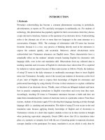
Fig. 1. (a) Thevenin noise model of resistor. (b) Norton noisemodel of resistor.

Fig. 2. (a) Parallel RC network. (b) Single pole RC low-pass
filter.

where IC is Boltzmann's constant, T is the absolute temperature, R is the resistance, and A f is the bandwidth in hertz
over which the noise is measured.
The power in thermal noise is proportional to the square
of Vt which is independent of frequency for a fixed bandwidth. The power between 100 and 200 Hz is the same as
it is between 10100 and 10200 Hz. Such noise is said to

have a uniform orflat power distribution and is called white
noise. It is called this by analogy to white light which also
has a flat power distribution in the optical band.
Equation (1) is the basis for two resistor noise models-the Thevenin model and the Norton model. These are
shown in Fig. 1. The short-circuit rms thermal noise current
in the Norton model of Fig. l(b) is given by

be modeled by a Gaussian or normal probability-density
function. For a Gaussian random variable, the probability

Because noise is random, the source polarities in the figure
are arbitrary. In general, the polarities must be labeled when
writing circuit equations. The total rms noise in a circuit is
independent of the assumed polarities.
Thermal noise is present in all circuit elements containing
resistance. The noise is independent of the composition of
the resistance. It is modeled the same way in discrete-circuit
resistors and in integrated-circuit monolithic and thin-film
resistors [4]. A carbon composition resistor generates the
same amount of thermal noise as a metal film resistor of the
same value. However, an additional noise component called
flicker noise may be present in the carbon composition
resistor. It results from the variable contact between the
carbon particles of the resistive material. This noise is
present only when a direct current flows in the resistor.
It is discussed in more detail in Section IV.
Equation (1) shows that thermal noise voltage is proportional to the square root of the product of the absolute
temperature, the resistance value, and (to the highest measurable frequencies) the bandwidth over which the noise
is measured. For a fixed temperature, the thermal noise
voltage in a circuit can be reduced by minimizing the

resistance and the bandwidth. Further reduction can only
be obtained by operating the circuit at lower temperatures.
The crest factor for thermal noise is defined as the ratio
of the peak value to the rms value. Although the rms
value can be calculated, the peak value cannot because
it is random. A common definition for the peak value is
the level that is exceeded only 0.01% of the time [5].
To relate this to the rms value, a statistical model for
the amplitude distribution is required. It is common to
assume that the amplitude distribution of thermal noise can
1516

that the instantaneous value exceeds four times the rms
value is approximately 0.01%. Thus the crest factor is
approximately 4.
In any circuit containing resistors, capacitors, and inductors, only the resistors generate thermal noise. (The
winding resistance of an inductor must be modeled as a
separate resistor.) Let 2 be the complex impedance of a
two-terminal network. The open-circuit rms thermal noise
voltage generated by the network in the frequency band
from f l to f 2 is given by

where Re ( 2 )is the real part of 2 and f is the frequency
in hertz. Let f 2 = f i Af. If A f is sufficiently small, the
noise voltage divided by the square root of the bandwidth
can be solved for to obtain

+

(4)

This equation defines what is called the spot noise voltage
generated by the impedance. The units are read "volts per
root hertz".
The total noise voltage generated by any resistor is
limited by its shunt capacitance. For a physical resistor,
this capacitance can never be zero. Figure 2(a) shows a
parallel RC circuit. The complex impedance and its real
part, respectively, are given by

2 = Rll(l/j27rfC) = R/(1 + j 2 7 r f R C )
and

Re(2) = R / [ l + (27rfRC)'I.
It follows from (3) that the total rms open-circuit thermal
noise voltage is given by

It can be concluded that the total noise voltage generated
by a resistor is a function only of the temperature and the
total shunt capacitance across the resistor.
PROCEEDINGS OF THE IEEE. VOL. 82, NO. IO. OCTOBER 1994


111. SHOTNOISE

Shot noise is generated when a current flows across a
potential barrier [l], [4], [5]. It is caused by the random
fluctuation of the current about its average value and occurs
in vacuum tubes and in semiconductor devices. In vacuum
tubes, it is generated by the random emission of electrons
from the cathode. In semiconductors, it is generated by

the random diffusion of holes and electrons through a p-n
junction and by the random generation and recombination
of hole-electron pairs.
The shot noise generated by a device is modeled by a
parallel noise current source. The rms shot-noise current in
the frequency band Af is given by

Ish =

J24laf

by the application of too large an input voltage. A diode
in parallel with the base-to-emitter junction is often used
to prevent it. For example, the MAT-02 and MAT-03 lownoise matched dual monolithic BJT pairs have the diodes
fabricated as part of the devices.
The power in flicker noise is proportional to the square
of I f which is inversely proportional to the frequency.
Because of this, flicker noise is commonly referred to as
l/f noise, read “one-over-f noise.” Because it increases
at low frequencies, it is also referred to as low-frequency
noise. Another name that is sometimes used is pink noise
[lo]. This name comes from the optical analog of pink
light which has a power density that increases at the longer
wavelengths, i.e., at the lower frequencies.

(6)

where q is the electronic charge and I is the dc current
flowing through the device. This equation was derived by
Shottky in 1928 and is known as the Shottky formula.

For a fixed bandwidth, the noise current is independent of
frequency so that shot noise has a flat power distribution,
i.e., it is white noise. It is commonly assumed that the
amplitude distribution of shot noise can be modeled by
a Gaussian or normal distribution. Therefore, the relation
between the crest factor and rms value for shot noise is the
same as it is for thermal noise.
IV. FLICKERNOISE
The imperfect contact between two conducting materials
causes the conductivity to fluctuate in the presence of a
dc current [4], [5]. This phenomenon generates what is
called Jicker noise or contact noise. It occurs in any device
where two conductors are joined together, e.g., the contacts
of switches, potentiometers, relays, etc. In resistors, it is
caused by the variable contact between particles of the
resistive material and is called excess noise [6]. Metal film
resistors generate the least excess noise, carbon composition
resistors generate the most, with carbon film resistors lying
between the two. Flicker noise in BJT’s occurs in the base
bias current. In FET’s, it occurs in the drain bias current.
Flicker noise is modeled by a noise current source in
parallel with the device. The rms flicker noise current in
the frequency band Af is given by

V. BURSTNOISE
Burst noise is caused by a metallic impurity in a p-n
junction [4], [5], [6]. Because it is caused by a manufacturing defect, it is minimized by improved fabrication
processes. When burst noise is amplified and reproduced
by a loudspeaker, it sounds like corn popping. For this
reason, it is also called popcom noise. When viewed on an

oscilloscope, burst noise appears as fixed-amplitude pulses
of randomly varying width and repetition rate. The rate can
vary from less than one pulse per minute to several hundred
pulses per second. Typically, the amplitude of burst noise
is 2 to 100 times that of the background thermal noise [5].
Burst noise in BJT’s is discussed in [ 113 and [ 121.
VI. NOISEBANDWIDTH
When a noise voltage is measured, the observed value
is dependent on the bandwidth of the measuring voltmeter
unless a filter is used to limit the bandwidth to a value that
is less than that of the voltmeter. It is common to use such a
filter in making noise measurements. The noise bandwidth
of a filter is defined as the bandwidth of an ideal filter which
passes the same rms noise voltage as the filter, where the
input signal is white noise [5], [6]. The filter and the ideal
filter are assumed to have the same gains.
To express the noise bandwidth of a filter analytically,
let A ( f ) be its voltage gain transfer function and let A0 be
the maximum value of [ A (f)I, where f is the frequency in
hertz. The noise bandwidth B in hertz is given by

(7)
where I is the dc current, n N 1, K f is the flickernoise coefficient, and m is the flicker-noise exponent. In
modeling J E T noise at low temperatures, n is not fixed
[7]. In modeling base-current flicker noise in the BJT, m
is typically in the range 1 < m < 3 [ti]. To simplify the
analyses in the following, it is assumed that n = m = 1 in
all flicker-noise equations. It is straightforward to modify
the results for other values of n and m.
In BJT’s, flicker noise can increase significantly if the

base-to-emitter junction is subjected to reverse breakdown
[9]. This can be caused during power supply turn-on or
LEACH: FUNDAMENTALS OF LOW-NOISE ANALOG CIRCUIT DESIGN

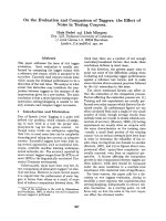
This equation is interpreted graphically in Fig. 3 for both a
low-pass filter and a band-pass filter. In each case, the actual
filter response and the response of an ideal filter having the
same noise bandwidths are shown. For the noise bandwidths
to be the same, the area under the actual filter curve must
be equal to the area under the ideal filter curve. For the
low-pass case, this makes the two indicated areas equal. A
similar interpretation holds for the band-pass case.
There are two classes of low-pass filters which are often
used in making noise measurements. The first has n real
poles, all with the same frequency. The second is an n1517


Fig. 3. Graphical interpretation of noise bandwidth for low-pass
and band-pass filters.

Table 1. Noise Bandwidth E of Low-Pass Filters
Number
of Poles

Slope
dB/dec

Real Pole

Butterworth

E

B

pole Butterworth filter. Table 1 gives the noise bandwidth
B for each filter as a function of the number of poles n
for 1 5 TI 5 5. For the real-pole filter, the noise bandwidth
is given as a function of both the pole frequency f o and
the upper -3-dB cutoff frequency f3. For the Butterworth
filter, the noise bandwidth is given as a function of the
upper -3-dB frequency. The table shows that the noise
bandwidth approaches the -3-dB frequency as the number
of poles is increased.
A simple R C low-pass filter such as the one shown in
Fig. 2(b) is an example single-pole filter that is often used
to limit the bandwidth of noise. This filter has the transfer
function A( f ) = 1/(1+j27r f R C ) . The pole frequency is
f o = 1/27rRC. From Table 1, the noise bandwidth is given
by B = 1.571/27rRC = 1/4RC.
Band-pass filters are used in making spot noise measurements. The filter bandwidth must be small enough so
that the input noise voltage as a function of frequency is
approximately constant over the filter bandwidth. The spot
noise voltage is obtained by dividing the filter noise output
voltage by the square root of its noise bandwidth. A filter
that is often used for these measurements is a second-order
band-pass filter. Such a filter has a -3-dB bandwidth of
fc/Q, where f c is the center frequency and Q is the quality
factor. The noise bandwidth is given by B = 7r fc/2Q. This
is greater than the -3-dB bandwidth by the factor ~ / 2 .

A single-pole high-pass filter cascaded with a singlepole low-pass filter is a special case of a band-pass filter
having two real poles. Let the pole frequency of the highpass filter be denoted by f l and that of the low-pass filter
be denoted by f 2 . The center frequency and the quality
factor of the band-pass filter are given by f c = (f1f2)lI2
and Q = f c / ( f l
f 2 ) . The noise bandwidth is given by
B = 7rfc/2Q = 7r( f l + f 2 ) / 2 . (Note that the frequencies fl
and f 2 are not the -3-dB frequencies of the filter. If the -3-

+

1518

dB frequencies are denoted by f a and f b , where f b > f a ,
the quality factor is also given by Q = f c / ( f b - fa).
Thus an alternate expression for the noise bandwidth is
B = T ( f b - fa)/2.>
The noise bandwidth of any filter can be measured
if a white-noise source and another filter with a known
noise bandwidth are available. With both filters driven
simultaneously by the white-noise source, the ratio of the
noise bandwidths is equal to the square of the ratio of
the output voltages. If VI is the rms noise output voltage
from a filter with the known noise bandwidth B1 and
V2 is the rms noise output voltage from a filter with the
unknown noise bandwidth B2, it follows that Bz is given
by B2 = B1(V2/Vd2.

VII. MEASURINGNOISE
Noise is normally measured at an amplifier output where

the voltage is the largest and easiest to measure [ 5 ] , [61,
[lo]. The output noise is referred to the input by dividing
by the gain. In measuring individual devices, a test fixture
can be used to hold the gain constant by use of negative
feedback [13]. The measuring voltmeter should have a
bandwidth that is at least ten times the noise bandwidth of
the circuit being measured [5]. If the voltmeter bandwidth
is insufficient, a filter with a known noise bandwidth can
be used preceding the voltmeter to limit the bandwidth to
a known value.
The voltmeter crest factor is the ratio of the peak input
voltage to the full-scale rms meter reading at which the
intemal meter circuits overload. For a sine-wave signal, the
minimum voltmeter crest factor is
For noise measurements, a higher crest factor is required. For Gaussian noise,
a crest factor of 3 gives an error less than 1.5%. A crest
factor of 4 gives an error less than 0.5%.To minimize errors
caused by an inadequate crest factor, measurements should
be made on the lower one-third to one-half of the voltmeter
scale to avoid overload on the noise peaks.
A true rms voltmeter is preferred over one which responds to the average reqtified value of the input voltage
but has a scale calibrated to read rms. When the latter type
of voltmeter is used to measure noise, the reading will be
low. For Gaussian noise, the reading can be corrected by
multiplying the measured voltage by 1.13.
Fairly accurate rms noise measurements can be made
with an oscilloscope [14]. A filter must be used to limit
the noise bandwidth at its input. Although the procedure is
subjective, the rms voltage can be estimated by dividing the
observed peak-to-peak voltage by the crest factor [5]. One

of the advantages of using the oscilloscope is that nonrandom noise which can affect the measurements can be
identified, e.g., a 60-Hz hum signal.
One method is to display the noise simultaneously on
both vertical channels of a dual-channel oscilloscope that
is set in the dual-sweep mode. The two channels must be
identically calibrated and the sweep rate must not be set too
high. The vertical offset between the two traces is adjusted
until the dark area between them just disappears. The rms

a.

PROCEEDlNGS OF TKE IEEE, VOL. 82, NO. 10, OCTOBER 1994


a7

The phasor output voltage V , is solved for by setting
V + = V - to obtain

vO

"t3

VO

-

Vt2

+I

Vt2

R+
2 R3)C
v, = Vtl 1 + j1~+(jwR2C

Q

R 3 Vt3

v-

This expression is converted into a root-square sum by
taking the square root of the sum of the squared magnitudes
as follows:

(b)

(a)

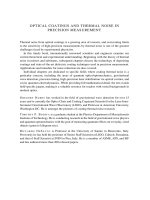
Fig. 4. Circuits used to illustrate addition of noise voltages.

"=

1

+ w2(R2+ R3)'C2
1 + W2R372

noise voltage is then measured by grounding the two inputs
and reading the vertical offset between the traces [15].
VIII. ADDITIONOF NOISEVOLTAGES

=

If the models for all noise sources are known, the
noise output voltage of a circuit can be calculated by the
methods of linear circuit analysis. The output voltage is
first calculated as if the instantaneous time-domain value
of each source is known. The rms value is then obtained
by converting the expression into a root-square sum.
To illustrate this, consider the circuit of Fig. 4(a) consisting of an ideal noiseless operational amplifier (op-amp) and
three resistors. Each resistor is modeled by its Thevenin
noise model, where the source polarity is arbitrary. Let
RE = RI R2 R3. The instantaneous op-amp input
voltages are given by

+

v+ = vti(R2

+

+ R3)/Rc + (ut2 + ut3 + vo)Ri/Rc

and
U-

= (uti - vt2)R3/RC

+

(

~

+3vo)(Ri+ Rz)/Rc.

The instantaneous output voltage is obtained by setting
U+ = w- to obtain v, = vtl
wt2(R1 R 3 ) / R 2- vt3. The
rms value of v, is obtained by converting the expression
into a root-square sum by taking the square root of the sum
of the squares as follows:

+

=

+

[licT(R1+ (Ri + R3)'
R2

+ R3) AS] 1'2

(9)

where the instantaneous voltages have been replaced by

the rms voltages. In squaring each term, all negative signs
disappear so that the result is independent of the source
polarities.
The preceding example illustrates noise calculations
when complex impedances are not involved. The circuit of
Fig. 4(b) is an example circuit with a complex impedance.
The circuit equations are written as if the noise voltages
were phasor quantities which are denoted here by bold face
letters. Let Z1 = R2 R3 l/jwC and 2 2 = R2 l/jwC,
where w = 2 n f . The op-amp phasor input voltages are
given V + = Vtl and V - = Vt2R3/Z1+(Vt3+Vo)22/Z1.

+ +

+

LEACH: FUNDAMENTALS OF LOW-NOISE ANALOG CIRCUIT DESIGN

[,,,(

R1

+ W2(R2 + R3)2C2
1 + w2R2C2

+ R2 1+Ww2R;C2
2R'C2 + R s ) A f ]

(11)

where the phasor voltages have been replaced by rms
voltages. This expression is a function of frequency. To
evaluate the noise voltage over a band, A f is replaced by
df and the quantity inside the brackets integrated over the
band. Alternately, the expression can be converted into a
spot noise voltage by dividing both sides by
In the examples presented above, two simplifying assumptions are made. First, it is assumed that the opamps are noiseless. This is not true for physical op-amps.
Second, it is assumed that the noise sources are statistically
uncorrelated. This assumption is valid when the noise
sources are independent of each other, e.g., when each noise
source represents the noise generated by a separate resistor.

m.

I x . THE vn-I, AMPLIFIERNOISEMODEL
The noise output from any amplifier is a function of the
noise generated by the source and the noise generated inside
the amplifier. An amplifier noise model can be obtained by
reflecting all internal noise sources to the input. In order
for the reflected sources to be independent of the source
impedance, two noise sources are required-a series voltage
source w, and a shunt current source in [16].
Figure 5(a) shows the amplifier noise model, where v,
is the instantaneous source voltage, Rs is the source resistance, and vts is the instantaneous thermal noise voltage
generated by Rs. The instantaneous output voltage is given
by

where A is the voltage gain and R; is the input resistance.
The equivalent noise input voltage is the voltage in series
with the amplifier input that generates the same noise

voltage at the output as all noise sources in the circuit.
It is denoted by U,; and is given by the sum of the noise
terms in the parentheses in (12).
1519


measure I,, V,, is measured with a large value resistor
for Rs (ideally Rs = 00) and I , is calculated from
(17). In measuring V,,, it is common to use a filter with
a known noise bandwidth preceding the voltmeter. The
measurements can be converted to spot-noise values by
dividing by the square root of the filter noise bandwidth.

x. THE SIGNAL-TO-NOISERATIO
The decibel signal-to-noise ratio (SNR) of the amplifier
of Fig. 5(a) is defined by

[

SNR = 2010g -

(c)

(b)

Fig. 5. (a) \;-I,, amplifier noise model. (b) Source with shunt
resistor across output. (c) Thevenin equivalent circuit of source
and shunt resistor.

= 101og

The rms value of v,; is obtained by taking the square
root of the time average of

+ v~,('u, + i,Rs) + U: + v,i,Rs + i:Rg.

~ 2=
i ut",

Because the noise generated by Rs is independent of the
noise generated by the amplifier, the average value of the
term uts (U, +in Rs) is zero. However, it cannot be assumed
that the average value of w,i, is zero. This is because one
or more noise sources in the amplifier might contribute to
both w, and in. In this case, the correlation coefficient p
between w, and i, must be known. This is defined by
1

P

(13)

-(.nin)

VnIn

where (vain)represents the time average of
value of wni is then given by

V,, = \/41cTRsAf

TJ,~,.

The rms

+ V: + 2pV,I,Rs + I:Rg.

172

1

"S

+ + 2pV,I,Rs + I;Rg]'

14kTRsA.f V:

(18)
The source resistance which maximizes the SNR is Rs = 0.
Although the source resistance is normally fixed, it can be
concluded that a series resistor should not be connected
between a source and an amplifier if noise performance is
a design criterion.
Figure 5(b) shows a source with a shunt resistor connected across its output terminals. To investigate the effect
of this resistor on noise, a Thevenin equivalent circuit of
the source and shunt resistor is first made. The circuit is
shown in Fig. 5(c), where v t l is the instantaneous thermal
noise voltage generated by the effective source resistance
RsllR1. With this circuit connected to the amplifier input in Fig. 5(a), it follows by analogy to (12) that the
instantaneous output voltage is given by

v, =

ARi

(14)

The correlation coefficient can take on values in the
range -1 5 p 5 fl. For the case p = 0, the sources
are said to be uncorrelated or independent. For Rs very
small, V,, N V, and the correlation coefficient is not
important. Similarly, for Rs very large, V,, N I,Rs and
the correlation coefficient is again not important. Unless
it can be assumed that p = 0, the Vn-In amplifier noise
model can be cumbersome for making noise calculations.
For the case p # 0, it is often simpler to use the original
circuit with its internal noise sources.
With w, = 0 in (12), the rms noise voltage at the amplifier
output is given by

vno-

z i ]

r

The equivalent noise input voltage in series with the amplifier input is given by the sum of the noise terms in the
parentheses in this equation.
The source voltage in (19) is multiplied by the factor
R1/(Rs R I ) . To define the instantaneous equivalent
noise input voltage referred to the source, this term must

be factored from the brackets. When this is done, TJ, is
given by

+

21,

=

ARi
R1
xRsllRi Ri Rs + R I

+

ARa J4kTRSAf+V~+2pVnInRs+I:R~.
Rs + R,

--

(15)
This equation can be used to solve for V, and I , as
functions of V,, to obtain

Vno
v, = A'

for Rs = 0

(16)

With the exception of the w, term, all terms in the brackets
in this expression represent the equivalent noise input
voltage referred to the source. Let this be denoted by wni,.
The rms value is given by

These equations suggest methods for measuring V, and
I,. To measure V,, V,, is measured with the amplifier
input terminals shorted and V, is calculated from (16). To
1520

PROCEEDINGS OF THE IEEE. VOL. 82, NO. 10, OCTOBER 1994


The amplifier SNR is given by SNR = 2010g (V,/V,;,).
This is maximized when Vnis is minimized. The value of
RI which minimizes this is RI = CO. For this value, the
SNR expression reduces to the one in (18). When noise is
a design criterion, it can be concluded that a resistor should
not be connected in parallel with an amplifier input unless
the resistor value is large compared to the source resistance.
Both the equivalent noise input voltage U,; and the
equivalent noise input voltage referred to the source u,is
are defined above. These two voltages are the same if the
source is connected directly to the amplifier input terminals.
If a coupling network is used between the source and the
amplifier, e.g., a bias network, the two voltages are not
necessarily the same. In general, to minimize the noise
for a particular design, the rms value of v,is should be
minimized. This always maximizes the SNR. In the event

that u,i = v,is, the noise is minimized by minimizing the
rms value of u,i.
A bias network consisting of a series element and a
parallel (or shunt) element is often required between a
source and an amplifier input. From the preceding results,
it can be concluded that the series impedance of the bias
network should be small compared to Rs and the shunt
impedance should be large compared to Rs.For example,
a series resistance of Rs/20 and a shunt resistance of 20Rs
can result in a decrease in the SNR by no more than 0.45
dB .

XI. NOISE FIGURE
The decibel noisefigure (NF) [5], [6] of an amplifier is
defined as the difference between its SNR and the SNR if
the amplifier were noiseless. It follows from (1 8) that the
noise figure for the amplifier model of Fig. 5(a) is given by

A noiseless amplifier has an NF of 0 dB. The value of
Rs which minimizes the noise figure is called the optimum
source resistance. It is given by Rso = Vn/I,. If a signal
source has an output resistance Rs that is not equal to the
Rso for an amplifier, a resistor should never be connected
in series or in parallel with the source to minimize the NF
because this decreases the SNR. However, if Rs can be
transformed to make Rs = Rso, the NF can be decreased
and the SNR increased. Adding a transformer between the
source and the amplifier is a method of doing this that is
discussed in Section XIII.
The NF can be a very misleading specification. If an

attempt is made to minimize an amplifier NF by adding
resistors either in series or in parallel with the source, the
SNR is always decreased. This is referred to as the noise
figure fallacy [17]. Potential confusion can be avoided if
low-noise amplifiers are designed to maximize the SNR.
This is accomplished by minimizing the equivalent noise
input voltage referred to the source. The low-noise design
methods described in this paper are based on this approach.
LEACH: FUNDAMENTALS OF LOW-NOISE ANALOG CIRCUIT DESIGN

Fig. 6. Circuit used to illustrate noise reduction with parallel
devices.

INPUTDEVICES
XII. NOISEREDUCTIONWITH PARALLEL
A method which can be used to reduce the noise generated in an amplifier input stage is to realize that stage with
several active devices in parallel, e.g., parallel BJT's or
parallel FET's [6], [18]. This technique is commonly used
in low-noise op-amps. Figure 6 shows a simplified block
diagram of an amplifier input stage having N identical
devices in parallel. For simplicity, only the first two are
shown. The noise source ut, models the instantaneous
thermal noise generated by the source resistance Rs. Each
amplifier stage is modeled by the Vn-I, amplifier noise
model. The input impedance to each stage is modeled
by a resistor. The output circuit is modeled by a Norton
equivalent circuit consisting of a parallel current source
and resistor. The short-circuit output current from the
j t h stage can be written i,j = gmvij, where g m is the
transconductance and vij is the input voltage for that stage.

The instantaneous short-circuit output current from the
circuit can be written

To define the equivalent noise input voltage, the term
multiplying U, must be factored from the outer brackets
in this equation. All remaining terms with the exception of
the w, term then represent w,i. When this is done and the
expression for u,i is converted into a root-square sum, a
significant simplification occurs. The final expression for
V,, is

Vni =

\i

4kTRsAf

1
+ -V:
+ 2pV,InRs + NIZR;
N

(24)
where p is the correlation coefficient between U, and in for
any one of the N identical stages.
If Rs = 0, (24) reduces to Vni = V,/fi. In this case,
the noise can theoretically be reduced to any desired level
if N is made large enough. For Rs # 0, (24) predicts that
1521

Fig. 8.

Diagram of multistage amplifier.

Because the series resistance of a transformer winding
is proportional to the number of turns in the winding, it
follows that R z / R 1K n. This makes it difficult to specify
the value of n which minimizes Vnis.In the case that
Rs >> R1 R2/n2, the expression for Vnisis given
approximately by

+

(b)

Fig. 7.

(a) Signal source coupled to amplifier through ideal
transformer. (b) Amplifier with equivalent input circuit.

Vnis

Vni -+ 0;) for N + 0 or N 00. Thus there is a value of
N that minimizes the noise. It is given by

/4A:TRs A f

1
+2

V; + 2pVn I,, Rs + I:nz R t .
(28)

---f

N = - Vn
1
7
%
RS

n=

This expression shows that N decreases as Rs increases.
It follows that the noise cannot be reduced by paralleling
input devices if the source resistance is sufficiently large.
XIII. NOISE REDUCTIONWITH

AN

INPUTTRANSFORMER

A transformer at the input of an amplifier may improve
its noise performance. Figure 7(a) shows a signal source
connected to an amplifier through a transformer with a turns
ratio 1 : n. Resistors R1 and Rz,respectively, represent the
primary and the secondary winding resistances. Figure 7(b)
shows the equivalent circuit seen by the amplifier input
with all noise sources shown. The source vtl represents the
thermal noise generated by the effective source resistance

n2(Rs RI) R2. By analogy to (12), the instantaneous
amplifier output voltage is given by

+

This is minimized when n is given by

+

The equivalent noise input voltage referred to the source
is obtained by factoring the turns ratio from the brackets
in (26) and retaining all terms except the w, term. The
expression obtained can be converted into a root-square
sum to obtain

/=.

In Rs

(29)

In this case, the effective source resistance seen by the
amplifier is n2Rs = Vn/In. This is the optimum source
resistance that minimizes the NF. Thus the NF is minimized and the SNR is maximized simultaneously by the
transformer.
The transformer winding resistance can be a significant
contributor to the thermal noise at the amplifier input,
especially if the source resistance is small. For this reason, a
transformer can result in a decreased SNR compared to the
case without the transformer [ 191. With a BJT input stage,

it is shown in Section XVI that the noise can be minimized
by biasing the input stage at a particular current. When this
is done, a transformer cannot be used to decrease the noise
further.
XIV. NOISEIN MULTISTAGE
AMPLIFIERS
Multistage amplifiers are commonly analyzed by considering only the noise sources in the input stage. The
conditions under which this is valid are discussed in this
section. Figure 8 shows a simplified diagram of a multistage
amplifier having N stages. For simplicity, only the first
two are shown. The instantaneous equivalent noise input
voltage for each stage is shown as a series voltage source
preceding that stage. The input impedance to each stage is
modeled by a resistor. Each output circuit is modeled by
a Norton equivalent circuit consisting of a parallel current
source and resistor.
The short-circuit output current from the j t h stage can be
written , ,z = G,Jv,,(oc), where v,J(oc)is the open-circuit
input voltage and G,, is the transconductance gain from
the open-circuit input voltage to the short-circuit output
current. The latter is given by G,, = gm,Rz,/(Ro(,--l)
Rz,), where ,g is the ratio of the short-circuit output
current to the actual or loaded input voltage. The opencircuit voltage gain of the j t h stage is given by G,, R,, .
The overall voltage gain of the circuit can be written

+

where p is the correlation coefficient between vn and in.
1522

PROCEEDINGS OF THE IEEE, VOL. 82, NO. IO, OCTOBER 1994


the root-square sum

I,
(a)

(b)

Fig. 9. (a) Noise model of diode. (b) Small-signal noise model
of diode.

It is straightforward to show that the output voltage is given
by

+...+

VniN

1-

GmiRoiGm2R02.. . Gm(hr-l)Ro(N-i)

(30)
The equivalent noise input voltage v,i is given by the
sum of all terms in the brackets in this equation except the
v, term. In the expression for wni, the equivalent noise input
voltage of the second stage is divided by the open-circuit
voltage gain of the first stage, that of the third stage is

divided by the product of the open-circuit voltage gains of
the first and second stages, etc. If the open-circuit voltage
gain of the first stage is high enough, the dominant term
in the expression for vni is un;l. It follows that the noise
performance of a multistage amplifier can be analyzed by
considering only the noise sources in the input stage if
the input stage gain is sufficiently high. This condition is
assumed to hold in most of the examples presented in the
following.

=

i

2qIAf

+ Kf1a.f
f
~

where it is assumed that I >> Is. A plot of I, versus
f for a constant A f exhibits a slope of - 10 dB/decade
for very low frequencies and a slope of zero for higher
frequencies. The two terms under the radical in (32) are
equal at the frequency where the noise current is up 3
dB compared to its high-frequency limit. This frequency
is called the Picker-noise comer frequency. A knowledge
of the flicker-noise comer frequency f f for a diode can be
used to calculate the flicker-noise coefficient. It is given by

Diodes are often used as noise sources in circuits. Specially processed Zener diodes are marketed as solid-state
noise diodes. The noise mechanism in these is called
avalanche noise and it is associated with the diode reverse
breakdown current [4]. For a given breakdown current,
avalanche noise is much greater than the shot noise in the
same current. Avalanche noise diodes have a typical noise
density of 0.05 pV per root hertz over the frequency range
from 10 Hz to 10 MHz [20].
XVI. THE BJT NOISE MODEL

The noise analyses of the BJT common-emitter (CE),
common-base (CB), and common-collector (CC) amplifiers
are given in this section. The load voltage for each amplifier
is proportional to the short-circuit output current. This current is calculated for each configuration, and the expression
for the equivalent noise input voltage is obtained. The
xv. THE JUNCTION-DIODE
NOISE MODEL
conditions for optimum noise performance are identified.
The principal noise sources in a BJT are thermal noise in
The current in a p-n junction diode consists of two
components-the
forward diffusion current I F and the
the base spreading resistance, shot noise and flicker noise
in the base bias current, and shot noise in the collector bias
reverse saturation current I S . The total current is given by
I = 1, - I s . The forward diffusion current is a function of
current [l], [4], [21], [22]. The small-signal T-model is used
the diode voltage V and is given by IF = IS exp ( V / ~ V T ) , here to calculate the effect of these. Figure 10(a) shows the
where 7 is the emission coefficient and V, is the thermal
T-model with the collector node grounded and all noise

voltage. (For discrete silicon diodes 7 E 2 whereas for
sources shown. The short-circuit collector output current
integrated circuit diodes 7 ‘v 1.) Both I F and I S generate
is labeled ic(sc). The circuit contains two signal sources,
uncorrelated shot noise. The total shot noise can be written
one connects to the base (vi and R 1 )and the other to the
as a root-square sum of the two shot-noise components and
emitter (v2 and R2). With w2 = 0, the circuit models a CE
is given by
amplifier. With v1 = 0, it models a CB amplifier.
In the figure, r, is the base spreading resistance, a is
In = d2q(IF 1s)A.f
the emitter-to-collector current gain, r o is the collector-toemitter resistance, and re is the intrinsic emitter resistance.
The latter is given by re = QVT/IC,where V, is the
‘v J 2 q I A f
(31)
thermal voltage and IC is the collector bias current. The
collector-to-emitter resistance is given by r, = (VCB
where the approximation holds for a forward-biased diode
for which I >> I S . Figure 9(a) shows the diode noise
V A ) / I c ,where VCB is the collector-to-base bias voltage
model. In Fig. 9(b), the diode is replaced by its small-signal
and VA is the Early voltage. The collector, emitter, and
resistance rd = vVT/(I I s ) E qVT/I. The small-signal
base bias currents are related by IC = a l =~ ~ I Bwhere
,
open-circuit rms noise voltage across the circuit is given
p = a/(1- a).
by Vn = Inrd.
The noise sources uti, wtz, and vt2, respectively, model

the instantaneous thermal noise in R I , r,, and R2. The
At low-frequencies, the diode exhibits flicker noise.
When this is included, the total noise current is given by
instantaneous shot noise and flicker noise, respectively, in

+

+

+

LEACH: FUNDAMENTALS OF LOW-NOISE ANALOG CIRCUIT DESIGN

1523


If i , is neglected, zc(s,-)
Fig. 10(b) to obtain

v1

Q

can be written by inspection from

It is convenient to define the BJT transconductance gain
G , by

-

G, =

Q

+ + + R2 .

(1 - a)(R1

T,)

(35)

Te

With this definition, (34) can be written

The terms in the parentheses in (36) represent the instantaneous equivalent noise input voltage. The expression for
u,i can be reduced to

-

(b)

Fig. 10. (a) T-model of BJT with noise sources shown. (b)
Equivalent circuit used to solve for i c ( s c l .

This can be converted into a root-square sum over the band
Af to obtain

4kT(R1+ T ,

+ R2)Af

I B are modeled by ishb and by i f b . The instantaneous shot
noise in IC is modeled by i s h c . In the band A f , the rms
values of the noise sources are given by

V,, = ( 4 / ~ T R l A f ) l / ~
V,,

Ifb

= (4kT~,Af)l/~

= (Kf1BA.f/ f ) 1 / 2

4kT(R1+ T ,

and

Ishc = ( 2 q I ~ A . f ) ~ ’ ~ .
Figure 10(b) shows an equivalent circuit with Thevenin
equivalents made of the noise sources in the base and
emitter circuits. Because the left node of the ai’,-controlled
source is disconnected from the circuit and connected to
ground, the resistors in the base lead must be multiplied
by (1 - a ) in order for the voltage drops across them
to be the same. The noise sources
and w,, are given
by unb = ut1 W t ,

(ishb
Zfb)(RI T,) and ‘he=
ut2
(i& - ish(, - i f b ) & . The currents ik, i,, and zc(sc)
in this circuit are the same as in the circuit of Fig. 10(a).
The short-circuit output current in Fig. 10(b) is given by
zc(sc) = i s h c
ai’, i o . It will be assumed here that the
resistor T , is large enough so that the current i , can be
neglected in calculating zc(sc). This is an approximation that
leads to very little error in practice for the dominant effect
of T , is to set the small-signal collector output resistance.

+

+

+

1524

This expression gives the rms equivalent noise input voltage
for both the CE and the CB amplifiers. The SNR for either
amplifier is given by SNR = 2010g (&/Vni),
where & is
the rms value of w1 for the CE amplifier and the rms value
of w2 for the CB amplifier.
Except at low frequencies, the flicker-noise term in (38)
can be neglected. When this is done, V,; can be written

+

+

+

+

+2

+ R2)Af

+ + R2)’
RI + r, + R2
+

~P ~ A(R1
. f

T,

I‘,“

IC

112

. (39)

It can be seen that Vni + cx if IC + 0 or if IC + ca.

It follows that there is a value of IC which minimizes V,i.
This current is called the optimum collector bias current
and it is denoted by I c ( ~ ~ It~ is
) . given by
IC(0pt)

=

vT

Rl+r,+R2

x

~

P

m‘

(40)

let the equivalent
When the BJT is biased at
noise input voltage be denoted by Vni
It is given by

PROCEEDINGS OF THE IEEE, VOL. 82. NO. 10, OCTOBER 1994

0

15

I

1

1

10

ill
m
e

4 2

>

4 5
102

104

io3
Current Gam

Fig. 11. Plot of decibel change in

01

'C/'C(apt)

Vnz( m i n ) versus P for BJT.

Fig. 12. Plot of tkz/lL2(,,,,,,) in decibels versus I ~ / l c ( , , ~ )
for BJT with a-,3 = 100; b 3 = 1000; and c-/3 = 10 000.

For minimum noise, this equation shows that the series
resistance in the external base and emitter circuits should
be minimized and that the BJT should have a small T, and
a high /3.
Although Vni(min)
decreases as p increases, the sensitivity is not that great for the range of /3 for most BJT's.
Figure 11 shows a plot of the decibel change in V,; ( m i n )
as a function of /3 for 100 5 /3 5 10 000, where the 0-dB
reference level corresponds to 0 = 100. Most BJT's have
a /3 in the range 100 5 /3 5 1000. As p increases over this
range, Vni(min) decreases by 0.32 dB. Superbeta transistors
have a /3 in the range 1000 5 p 5 10 000 [6]. As p
increases over this range, Vni(min) decreases by only 0.096
dB. It can be concluded that only a slight improvement in
noise performance can be expected by using higher ,b' BJT's
when the device is biased at IC (opt).
If IC # IC (opt), Vn;can be written

(42)
Example plots of V,;/V,;
versus I c / I c (opt) are given

in Fig. 12, where a log scale is used for the horizontal axis.
Curve a is for ,O = 100, curve b is for ,6' = 1000, and curve
c is for /3 = 10 000. The plots exhibit even symmetry about
the vertical line defined by I ~ / l c ( , , , ~=) 1. This means,
for example, that V,; is the same for IC = IC (opt) / 2 as
for IC = 2Ic (opt). In addition, the figure shows that the
sensitivity of V,; to changes in IC decreases as /3 increases.
For example, at IC = IC
and IC = 2Ic (opt), V,i is
greater than
by 0.097 dB for ,l3 = 100, by 0.033
dB for ,O = 1000, and by 0.010 dB for @ = 10 000.
Noise specifications for BJT's commonly give measured
values for V, and I , for the
amplifier noise model.
To solve for the theoretical expressions for these, (37) can
be written U,; = wtl - vt2 U ,
& ( R I T,
R2),
where U, and 2, are given by U, = ut,
ishcVT/IC
and in = i s h b i f b ishc/@.These expressions can be
converted into root-square sums to obtain

+ +

+

+ +
+

+

4kTr,Af i - 2 k T 5 A f
IC

+

2 q I ~ A f -Af
Kf IB

f

(43)

+ -Af.
29Ic

(44)

P2

LEACH: FUNDAMENTALS OF LOW-NOISE ANALOG CIRCUIT DESIGN

D

C

E

(a)

D

S

(C)

(b)

Fig. 13. (a) lil-In noise model for BJT. Asterisk indicates that
rf is noiseless, i.e., its noise is included in v , ~ (b)
. Model for
J E T . (c) Model for MOSFET.

Because ishc appears in both expressions, the correlation
coefficient for U, and i, is not zero. If it is assumed that
ishb. z f b , and zshc are not correlated, (13) can be used to
show that the correlation coefficient for w, and in is given
by
(45)
The V,-I, BJT noise model is shown in Fig. 13(a). The
asterisk indicates that the base spreading resistance T ; is
considered to be a noiseless resistor.
Equation (44) predicts that a plot of I , versus frequency
would exhibit a slope of - 10 dBIdecade at low frequencies
and a slope of zero at higher frequencies. The Picker- noise
corner frequency f f for I, is the frequency at which I, is
up 3 dB compared to its higher frequency value. This is
the frequency for which the center term in the radical in

(44) is equal to the sum of the first and last terms. If this
frequency is known for a BJT, the flicker-noise coefficient
can be solved for. It is given by
K f

= 2 g f f (1

+j).

(46)

The base spreading resistance T , is a difficult parameter
to measure. This is because T, is a distributed, variable
resistance that is modeled as a lumped-constant resistance.
Its value can range from approximately 10 R for microwave
devices to over several kilohms for lower frequency devices
[23]. There are several methods for measuring T, which
generally give different values. For this reason, a noise
152.5


measurement technique should be used if r, is to be used
in noise calculations [23]. As an example, the LM194
and LM394 are precision matched monolithic n-p-n BJT
pairs. These are specified to have a noise equivalent base
spreading resistance of 40 R [24]. This low value of r,
is accomplished by fabricating each BJT as a number of
parallel devices. The design of a low r, BJT is discussed
in [25].
The above analysis shows that the noise performance of

the CE amplifier is the same as the CB amplifier. This
assumes that the noise generated by the BJT collector load
can be neglected. When the load noise is included, this
conclusion may no longer be true. To investigate this, let
the short-circuit rms noise current generated by the collector
load be denoted by I,t. To account for this noise in (38),
the term I:€/G; must be added inside the brackets, where
G, is given by (35).The effect of I,€ on the two amplifiers
can be compared by comparing the values of G, for three
cases. For the CE amplifier, let R1 = Rs, R2 = 0, and
denote G , by G, (cE). For the CB amplifier, let RI = 0,
RZ = Rs, and denote G, by G,(cB). The ratio of
G,(cE) to G,(cB) is given by

Gm (CE)
-Gm (CBI

-

+ +

( 1 - a ) ~ , re Rs
( 1 - ~ ) ( R srz) r e

+

+

(47)
'

For Rs = 0, the ratio is unity. In this case, the effect of
I,t on the two amplifiers is the same. For Rs large, the
ratio approaches 1/(1 - a ) = 1 p so that the effect of
I,€ in the CB amplifier is greater than in the CE amplifier.
Therefore, the CE amplifier is the preferred topology for
low-noise applications when the source resistance is not
low. This conclusion is dependent on the assumed values
for R1 and Rz in the expression for G,.
The CC amplifier is often used as a unity-gain buffer
between a source and an amplifier. Figure 14 shows the
circuit diagram of a CC amplifier with its output connected
to the input of a second stage that is modeled with the
V,-I, amplifier noise model. For simplicity, the bias
sources are not shown. The resistor r, and all BJT noise
sources are shown external to the BJT. The source it2
models the thermal noise current in Rz. The voltage across
R; is proportional to the short-circuit current through R;,
i.e., the current i ; evaluated with Ri = 0. It is given by

+

where G, is given by (35) with R2 = 0. It follows that the
instantaneous equivalent noise input voltage is given by

1526

AV;

Fig. 14. BJT CC stage connected between signal source and

amplifier input.

This can be converted to a root-square sum to obtain

4kT(R1+rX)Af
+V:Af +2pV,I,Af

where p is the correlation coefficient between U , and i, and
it is assumed that V, and I, are for a bandwidth Af = 1
Hz.
It can be seen from (48) that the V, noise appears directly
at the input. The I, noise is multiplied by ( R I r,)/(l
p) aVT/Ic. If this is less than R1, the CC amplifier
reduces the effect of the I, noise compared to the case
where the source is connected directly to the second stage.
The noise voltage generated by the base shot- and flickernoise currents is independent of the load resistance R; and
can be canceled if RI r, - &/IC = 0. For the case
R2 = 2kT/qIc, the collector shot noise and the thermalnoise current generated by R2 have equal contributions. For
R2 >> 2kT/qIc = O.O518/Ic, the noise generated by R2
can be neglected.

+

+

+

+

AMPLIFIERS

XVII. NOISEIN SERIES-SHUNT FEEDBACK
The advantages of negative feedback in amplifier design
are well known. This section illustrates the noise analysis
of a series-shunt amplifier where the signal source is
modeled as a voltage source, e.g., a low output-impedance
transducer. The input stage is assumed to be a BJT CE
stage. The methods used are applicable to other input stages.
Figure 15(a) shows the simplified diagram of the amplifier with the BJT input stage explicitly shown. The bias
sources and networks are omitted for simplicity. This is
an example circuit where the BJT is both a CE amplifier
and a CB amplifier. It acts as a CE amplifier for the signal
source and a CB amplifier for the feedback signal. If the
loop gain is sufficiently high, the small-signal voltage gain
is approximately the reciprocal of the feedback ratio and is
given by I J , / ~ J ~
1 RF/RE.
The circuit in Fig. 15(b) can be used to solve for the
equivalent noise input voltage. The figure shows the BJT
with its collector connected to signal ground and the circuit
seen looking out of the emitter replaced by a Thevenin

+

PROCEEDINGS OF THE IEEE. VOL. 82, NO. 10. OCTOBER 1994


'S

(a)

,s@m$c
@!t?vo
~.~

-~
.
.

(a)

(b)

~

R2

(b)

Fig. 15. (a) Series-shunt amplifier. (b) Noise equivalent circuit

Fig. 16. (a) Shunt-shunt amplifier. (b) Noise equivalent circuit

of input stage.

of input stage.

equivalent circuit with respect to U , . The instantaneous
equivalent noise input voltage is modeled by the source
w,i. If flicker noise is neglected, the rms value of w,i is
obtained from (39) with R2 replaced with REIJRF.It is

given by
r

~.

Fig. 17. BJT diff-amp with noise sources

(49)
Equations (38) and (40)-(46) also apply with R2 replaced
with REJIRF.
For minimum noise, REIJRF should be small compared
The
to R1 r, and the BJT should be biased at Ic(opt).
resistance REIJRFcannot be zero because the amplifier
gain is set by the ratio of RF to RE.If the BJT is biased at
Iccopt)and R E ~ ~ =
RF
R1 T,, it follows from (41) that
the noise is 3 dB greater than for the case where the BJT
is biased at Zc (opt) and R ~ lRF
l = 0. Note that the value
of Zc(opt) is different for the two cases.

+

+

XVIII. NOISEIN SHUNT-SHUNT FEEDBACK
AMPLIFIERS
This section illustrates the noise analysis of a shunt-shunt

amplifier. The signal source is modeled as a current source,
e.g., a high output-impedance transducer. The amplifier
input stage is assumed to be a BJT CE stage. The methods
used are applicable to other stages.
Figure 16(a) shows the simplified diagram of the circuit
with the BJT input stage explicitly shown. The bias sources
and networks are omitted for simplicity. The signal source
is represented by the current source i s in parallel with
the resistor Rs. If the loop gain is sufficiently high, the
small-signal transresistance gain is given by w o / i s 21 -RF.
The circuit in Fig. 16(b) can be used to evaluate the inputstage noise performance. The figure shows the BJT with its
collector connected to signal ground and the circuit seen
looking out of the base replaced by a Norton equivalent
circuit with respect to is and U,. The instantaneous equivalent noise input voltage is modeled by the source uni. The
short-circuit collector current i,
is given by

Because the signal source is a current as opposed to a
voltage, the noise equivalent input current i,i in parallel
with i s must be calculated. This is obtained by factoring
the coefficient of is from (50) and retaining only the
term involving w,i. It follows that in; is given by i,i =
v,i/RsllR~.When flicker noise is neglected, the rms value
of zlni is given by (39) with RI replaced with R ~ J I R F
It .
follows that the rms value of i,i is given by

(51)
The noise is minimized by making Rz small and by making
RF large compared to Rs. In addition, the BJT should be

biased at IC (opt).

XIX. BJT DIFFERENTIAL-AMPLIFIER
NOISE
The differential amplifier (diff-amp) is commonly used
as the input stage of op-amps. Figure 17 shows the circuit
diagram of a BJT diff-amp. For simplicity, the bias sources
are not shown. It is assumed that the BJT's are matched
and biased at equal currents. The emitter resistors labeled
R2 are included for completeness. For lowest noise, these
should be omitted. The source int models the instantaneous
noise current generated by the tail current source and the
resistor rt models its output resistance.
For minimum noise output from the diff-amp, the output
signal must be proportional to iCl(.Cl - ic2(.). The subtraction cancels the common-mode noise generated by the
. current int.Although a current-mirror active load can be
where G, is given by (35) with R1 replaced with R ~ ~ J R F tail

LEACH: FUNDAMENTALS OF LOW-NOISE ANALOG CIRCUIT DESIGN

1527


used to realize the subtraction, the lowest noise performance
is obtained with a resistive load. With a resistive load on
each collector, a second diff-amp is required to subtract
the output signals. The analysis presented here assumes
that the circuit output is taken differentially. In addition,
it is assumed that rt is large enough so that it can be
approximated by an open circuit. This is equivalent to the

assumption of a high common-mode rejection ratio.
The simplest method of analysis is to make use of the
results of Section XVI. This is done by solving for an
equivalent noise input voltage in series with each BJT base.
When solving for the input-noise voltage for one side of the
diff-amp, the other side is considered to be noiseless. Let
u T 2 i 1 be the instantaneous equivalent noise input voltage in
series with u,l which generates the same noise in irl
as
the noise generated by R 1 1 , Q 1 , and the R2 in series with
the emitter of Q 1 . Equation (37) can be used to solve for
w n i l . However, the equation must be modified to include
the effect of a noiseless resistor in series with the emitter
of Q 1 . This resistance is RZ T;,z, where r;,2 is the smallsignal resistance seen looking into the emitter of Q2. The
latter is given by Tie:! = ( 1 - a ) ( R 1 2 r,)
r,.
To modify (37), R 2 is replaced with 2 R 2 + r i e 2 . It follows
that ~ ~ is ~given
i
1by

+

+

unzl = u t 1 1

x

+

-

2R2

icl(sc)

= Gml(vs1

+ uni1)

and
-ishcl)/a

+ ishcl

-

ishbl

-

+ utx2 - ut22 + (ishb2 + i f b 2 )
x ( R 1 2 + T, + 2 R 2 + r i e l )

= ut12

f ishc2(1/Gm2

-

2R2

+

- riel)

+

where T,,I = ( 1 - a ) ( R l l r,)
r, is the small-signal
resistance seen looking into the emitter of Q1 and Gm2 is
given by (35) with RI replaced with R 1 2 and R 2 replaced
with 2 R 2 riel. The collector and emitter currents in Q 2
due to 71,2 and un;2 are given by

+

ic2(sc)

= Gm2(us2

+uni2)

and
ie2

=

(icZ (sc) - i s h c 2 ) / a

+ ishc2

-

ishb2

- ifb2.

By symmetry Gml = Gm2= C Y / ( T ; , I + 2 R ~ + r i ~ 2 ) which
,
is denoted by G, in the following.
I528

vs2

- wni2)

+ Q'(ishb2 + i f b 2 ) + (1

-

Ql)iShc2

+ aint/2

and
ic2 (se)

+ unt2 - vs1

+ a ( i s h b 1 + i f b l ) f (1

=Gm(us2

-

unil)

-

CY)ishcl

+ aint/2.

To define the overall instantaneous equivalent noise input
is formed
voltage uni, the difference current i e l ( s e- )i c 2
first. The coefficient of v , ~ u,2 is then factored from the
expression and all terms retained except the w s l - w,2 term.
When the result is converted into a root-square sum, the
following expression is obtained:

+R 1 2 / a +Tz + R 2
P

+

-

IC

21

1'2.

(52)

If R 1 1 = Rlz = RI, (52) reduces to fi multiplied by
(38). This is 3 dB greater than the equivalent noise input
voltage for the CE and CB amplifiers. Above the flickernoise frequency band, V,, is minimized when each BJT is
biased at a collector current given by

ifbl.

Let v n i 2 be the instantaneous equivalent noise input
voltage in series with vs2 which generates the same noise
in i c 2 (..I as the noise generated by R 1 2 , Q 2 , and the R 2 in
series with the emitter of Q 2 . By symmetry, it is given by
uni2

+ unil -

( R 11

- rie2)

+

( i c l (sc)

=Gm(vs1

7-x

where G,1 is given by (35) with RI replaced with R 1 1
and R 2 replaced with 2Rz r i e 2 . The components of the
collector and emitter currents in Q 1 due to w,l and w,il
are given by

=

i c l (se)

+ ut11 - u t 2 1 + ( i s h b l + i f b l )
+ + 2R2 + T i e 2 1

(R11

+ishcl(l/Gml

iel

The short-circuit collector output current for each side
of the diff-amp can be written as the sum of three components-the first is Gm(v,+vni) for that side of the diff-amp,
the second is -aie for the other side of the diff-amp, and
the third is crint/2, where it is assumed that ant divides
equally between the emitters of Q 1 and Q 2 . (This is strictly
true only if riel = rie2.)The two output currents are given
by

For R 1 1 = R I 2 = R1,this expression reduces to (40). The
rules for minimizing the diff-amp noise are the same as
those for the CE and CB amplifiers.
The LM38 1 low-noise dual monolithic preamplifier has
an input stage that gives the user the option of operating it
either as a diff-amp or as a single BJT stage. External leads
are provided which can be shorted to remove the second
transistor in the diff-amp from the circuit. When this is
done, the noise performance is improved by 3 dB [26].

XX. FREQUENCY
RESPONSEEFFECTS
This section presents two examples which illustrate frequency response effects in noise calculations. The first covers the low-frequency effect of a series coupling capacitor
at an amplifier input, The second covers the high-frequency
effects of the internal junction and diffusion capacitances
of a BJT on the noise performance of a CE amplifier.
The methods used in these two examples are applicable
in calculating frequency response effects in other circuits.
PROCEEDJNGS OF THE IEEE, VOL. 82. NO. 10, OCTOBER 1994


In general, the objective in a low-noise design is to
maximize the signal-to-noise ratio at an amplifier output.
This is given by SNR = 20 log ( V,,/V,,), where V,, is the
rms signal output voltage and V,, is the rms noise output
voltage. Let V,, = AV,, where V, is the rms source voltage
and A is the magnitude of the voltage gain, including
the gain of an input coupling network. It follows that the
SNR can also be written SNR = 20log(V,/V,,,), where
V,;, = V,,/A is the equivalent noise input voltage in series

with the source. For a fixed V,, the SNR is maximized
when V,;, is minimized. When frequency response effects
are considered, the gain A is a function of frequency. The
frequency at which A is evaluated should be the frequency
of the source. In some cases, this frequency may be different
from the frequency at which the noise is evaluated. This is
illustrated in the first example below.
Figure 18 shows an amplifier with an input coupling
network consisting of a series capacitor CI and a shunt
resistor R I . The V,-I, amplifier noise model is used for
the amplifier. The thermal noise sources for the resistors are
shown. To simplify the analysis, the correlation between
v, and i, will be neglected and it will be assumed that
R; >> R I . To calculate the amplifier input voltage, phasor
notation is used. By superposition, the input voltage is given
by

(54)
To calculate the equivalent noise input voltage referred to
the source, the expression for V;/V, must be factored from
this equation and all terms retained except the V, term.
The expression for V;/V, must be evaluated at the source
frequency, not the frequency of the noise. In circuits where
a series input coupling capacitor is used, the capacitor
is usually chosen to be large enough so that it can be
considered to be a short circuit at the source frequency (or
band of frequencies). In this case, Vi /V, = RI/(Rs R I ) .
When this is factored from (54), the rms equivalent noise
input voltage in series with the source can be solved for
to obtain

+

R,

"t-

C

Amplifier

v,

Fig. 18. Circuit used to illustrate effect of coupling capacitor on
low-frequency noise.

to decrease and the R1 and I , noise to increase but remain
finite as w + 0. The total noise voltage in any band can
be obtained by replacing Af with df and integrating the
expression inside the brackets over that band.
To illustrate the problems that occur if the incorrect
expression for Vi/V, is factored from the equation for
Vi, let V;/V, = R l / ( R s RI l/jwCl). This is the
general frequency-dependent expression for the gain. When
it is factored from the expression for V;, the following
expression for Vnis is obtained:

+

4kTRsAf

+

+ (4kTRlAf + V2Af

This expression predicts that the thermal noise generated by
Rs is independent of frequency even though there is a series
coupling capacitor between the source and amplifier. The
thermal noise generated by R1 and the V, and I , amplifier
noise are multiplied by the reciprocal of the square magnitude of a high-pass transfer function which approaches m
as w + 0. These observations certainly do not agree with
intuition. The problem is caused by factoring the incorrect
expression for V,/V, from the equation for V;.
The circuit in Fig. 19 is used for the second example
of frequency-response effects. The figure shows the circuit
diagram of a BJT CE amplifier in which the base spreading
resistance r,, the collector-to-emitter resistance r,, the
base-to-emitter diffusion capacitance c,, the collector-tobase depletion capacitance c,, and the BJT noise sources
are modeled as elements external to the transistor. For
simplicity, the bias sources are not shown. The base input
resistance is given by T, = (1 ,!3)r,. In writing the circuit
equations, phasor notation is used. The collector and base
currents can be written

+

r

where it is assumed that V, and I , are for a bandwidth
A f = 1 Hz. It can be seen that the thermal noise generated

by Rs is multiplied by the square magnitude of a high-pass
transfer function which approaches 0 as w
0. The V,
noise is independent of frequency. Both the thermal noise
generated by RI and the In amplifier noise are multiplied
by the square magnitude of a low-pass shelving transfer
function. It can be concluded that CI causes the Rs noise

to obtain

These equations can be solved for

+ Ishb + Ifb]

--f

LEACH: FUNDAMENTALS OF LOW-NOISE ANALOG CIRCUIT DESIGN

1

1

(R5+ %)llT,

+

1 +jw[(Rs rz)llr,](c,

+ c,)

- Ishc.

(58)
1529


Fig. 19. BJT CE amplifier used to illustrate high-frequency noise
calculations.

To calculate the equivalent noise input voltage referred to
the source, the coefficient of V , (evaluated at the frequency
of V , ) must be factored from (58) and all terms retained
except for the V , term. It will be assumed here that the
frequency of the source is equal to the frequency at which
the noise is calculated. In this case, the rms noise equivalent
input voltage can be written

(59)
where the time constant

T

is given by

It can be seen from this expression that the noise component
due to the collector shot noise increases at a rate of 20
dB/dec above the frequency defined by w = l / r . Thus
the signal-to-noise ratio given by SNR = 20 log (V,/Vnis)
decreases as frequency is increased above that frequency.
In reality, the high-frequency noise output from the circuit

approaches a constant whereas the signal approaches zero
as frequency is increased. Because (59) is derived under
the assumption that the frequency at which the noise is
evaluated is equal to the source frequency, the equation
cannot be used to calculate the noise at a frequency different
from that of the source.

XXI. THE FET NOISE MODEL
The noise models for the junction FET (JFET) and the
metal-oxide-semiconductor FET (MOSFET) are given in
this section. The principal noise sources in the FET are
thermal noise and flicker noise generated in the channel [ l ] ,
[4], [27]. For the JFET, this assumes that the gate current
is zero. Otherwise, shot noise in the gate current must be
included. Flicker noise in a MOSFET is usually larger than
in a JFET because the MOSFET is a surface device in which
the fluctuating occupancy of traps in the oxide modulates
the conducting surface channel all along the channel [l].
The relations between the flicker noise in a MOSFET and
its geometry and bias conditions depend on the fabrication
process [28]. In most cases, the flicker noise, when referred
to the input, is independent of the bias voltage and current
and is inversely proportional to the product of the active
1530

gate area and the gate oxide capacitance per unit area [4].
Considerations for the design of low-frequency low-noise
MOSFET amplifiers are discussed in [29]. Comparisons
of bipolar versus CMOS devices for low-noise monolithic
amplifier designs are given in [30].

Because the JFET has less flicker noise, it is usually
preferred over the MOSFET in low-noise applications at
low frequencies. Compared to the silicon JFET, the galliumarsenide (GaAs) JFET is potentially lower in noise [20].
However, the GaAs JFET can exhibit very high flicker
noise, making this device useful only for high frequencies.
Because the noise models for the JFET and the MOSFET
are essentially the same, the analyses presented in this
section apply to both.
It is assumed that the FET is biased in the saturation
region. The drain current is given by
ZD

= K(1

+

XUDS)(UGS

-

VTO)~

where WGS is the gate-to-source voltage, W D S is the drainto-source voltage, K is the transconductance parameter,
X is the channel-length-modulation factor, and VTO is
the threshold voltage. For the JFET, the transconductance
parameter is given by K = Ioss/V&, where IDSSis the
drain-to-source saturation current and V - 0 is also called
the pinchoff voltage. For the MOSFET, K is given by
K = p,C0,W/2L, where po is the average carrier mobility
in the channel (denoted by p, for the n-type channel and p?,

for the p-type channel), CO, is the gate oxide capacitance
per unit area, W is the effective channel width, and L is
the effective channel length [31].
Figure 20(a) shows the FET T-model with the drain node
grounded and all noise sources shown. For the MOSFET,
it is assumed that the small-signal bulk-to-source voltage is
zero so that the bulk lead can be omitted from the model.
The short-circuit drain output current is labeled id (.,-I.
There are two signal sources in the circuit, one connects
to the gate (111 and R I ) and the other to the source (712
and R2). With u2 = 0, the circuit models a CS amplifier.
With w1 = 0, it models a CG amplifier. The small-signal
transconductance is given by
gTn = 2[K(1+ \ X V D S ) I D ]2~ IKID)^/^
~

where I D is the drain bias current, VDS is the drain-tosource bias voltage, and the approximation assumes that
XVDs << 1. The drain-to-source resistor T , is given by
T o = (VDS
l/X)/rD.
The sources wtl and wt2, respectively, represent the
instantaneous thermal noise generated by RI and R2.
The rms values are V,, = (41CTR1af)~/~
and V,2 =
(4kTR2af)'/'. The source %,hg represents the instantaneous shot noise in the JFET gate current. The rms value
is given by 1 3 h g = ( 2 q I ~ A f ) l where
/ ~ , IG is the gate
bias current. This source is omitted in the MOSFET model.
In the properly biased JFET, I , consists of the saturation
current of the reverse-biased gate-to-channel junction. In

most applications, this is small enough so that it can be
neglected.

+

PROCEEDINGS OF THE IEEE,VOL. 82. NO. IO, OCTOBER 1994


It follows that (60) can be written

The instantaneous equivalent noise input voltage vni is
given by the terms in the parentheses in this equation. The
expression can be reduced to

This equation can be converted into a root-square sum over
the band A f to obtain

+

V,; = [4kT(R1+R2)A.f 2qIG((R1

+-3 4 k T m A’

Fig. 20. (a) Noise equivalent circuit of FET. (b) Circuit used to
solve for i d (..I.

The sources z t d and i f &respectively, represent the instantaneous thermal noise and flicker noise generated in
the channel. For both the MOSFET and the JFET, the
rms value of z t d is given by I t d = [4kT(2g,/3)Af]1/2.
For the MOSFET, the rms value of i f d is given by

I f , = ( K f I o A f / f L 2 C o , ) 1 /where
2 , a typical value for
the flicker noise coefficient is K f = lopz8 F . A [31].
For the JFET, the rms value of z f d is given by I f , =
( K f I o Af / f)’/’. The only difference in the equations for
I f d for the two devices is the absence of the L2 and CO,
terms in the JFET equation. It follows from the equation
for I t d that the rms thermal-noise current generated in
the channel is the same as the short-circuit thermal-noise
current generated by a resistor of value 3/29,.
Figure 20(b) shows an equivalent circuit with Thevenin
equivalents made of the noise sources in the external gate
and source circuits. The noise sources vng and w,, are
given by vng = v t l
ashgRl and v,, = vtz
(atd
i f d - ishg)&.The short-circuit drain current is given by
z d ( s c ) = ztd
zfd
i$ io. To simplify the calculation of
z d ( s c ) . it will be assumed that T , is large enough so that
the current io can be neglected. This approximation leads
to little error in practice because the dominant effect of T ,
is to set the small-signal drain output resistance. It follows
from Fig. 20(b) that
is given by

+

+

+

+

+ +

Let the transconductance gain G, for the FET be defined
by

+

Kf
Af]
4K f L2Co,

1/2

(64)

where 1, = 0 for the MOSFET and the L2 and CO,terms
are omitted for the JFET.
For minimum noise, it can be concluded from (64)
that the series resistance in the external gate and source
circuits should be minimized and the FET should have a
high transconductance parameter K and a low flicker-noise
coefficient K f . It can be seen that the channel thermal noise
decreases as the drain bias current increases. If all noise
except the channel thermal noise is neglected, (64) predicts
This decreases by 1.5 dB each time Io

that Vn; K
is doubled.
The JFET gate current is commonly assumed to be zero
when the gate-to-channel junction is reverse-biased. For a
high source impedance, the effect of the gate current on
the noise might not be negligible. In the design of lownoise JFET circuits, particular attention must be paid to
the variation of the gate current with drain-to-gate voltage.
In general, the gate current increases with drain-to-gate
voltage. Some devices exhibit a threshold effect such that
the gate current increases rapidly when the drain-to-gate
voltage exceeds some value. The drain-to-gate voltage at
which this occurs is called the IC breakpoint. It is typically
in the range of 8 to 40 V, depending on the particular
device [32].
For low-noise applications, the FET should have a high
transconductance parameter. For the JFET, this requires a
large drain-to-source saturation current and a small threshold or pinchoff voltage. As an example, the CD860 is
a dual-matched n-channel JFET pair that is specified as
an ultra-low-noise device having the typical parameters
IDSS = 100 mA, VTO= -1.5 V, and K = 4.4 x lop2
A N 2 . In contrast, the 2N54.57 is a general-purpose nchannel JFET having the typical parameters IDSS = 3 mA,
VTO= -3 V, and K = 3.3 x lop4 A N 2 .
Noise specifications for FET’s usually give measured
values for V, and I , for the &I, amplifier noise model.
To obtain theoretical expressions for these, (63) can be
written

p4.

vnZ = V t i - ut2

LEACH: FUNDAMENTALS OF LOW-NOISE ANALOG CIRCUIT DESIGN

+ R2)’A.f

+ + i,(R1 + R2)
V,

1531


+

where U n = (*&d ifd)/gm and in = z s h g . The rms values
for U, and in are given by

3 a A f

+

4K f Kf
L2C,, Af

(65)

where In= 0 for the MOSFET and the L2 and CO, terms
are omitted for the JFET. It is common to assume that i s k g
is independent of both it* and i f d . Thus the correlation
coefficient between vn and in is zero. Figure 13(b) shows
the V,--I, noise model for the JFET. Figure 13(c) shows the
model for MOSFET. The latter model is valid only when

the MOSFET small-signal bulk-to-source voltage is zero.
Measured V, data for typical NMOS and PMOS devices
are given in [31] and [32]. The devices described were
fabricated with a 6-pm, silicon-gate, p-well CMOS process.
The oxide thickness was 750 8, and the drain current for
all measurements was 45 pA. For the NMOS devices, the
flicker noise was found to be dominant below 10 kHz. For
the PMOS devices, it was found to be dominant below 1
kHz. At 100 Hz, a 100 p d 5 pm NMOS device was found
to exhibit a noise voltage of 680 nV per root hertz while
a corresponding PMOS device exhibited 120 nV per root
hertz. Thus the PMOS device noise was approximately 5
times less than the NMOS device noise.
It can be seen from (65) that a plot of V, versus frequency
would exhibit a slope of - 10 dB/decade at low frequencies
and a slope of zero at higher frequencies. Thejicker-noise
comer frequency ff for V, is defined as the frequency at
which V, is up 3 dB compared to its higher frequency
value. This is the frequency for which the two terms in the
brackets in (65) are equal. A knowledge of ff for a FET
can be used to calculate the flicker-noise coefficient K f .
It is given by

where the L2 and C,, terms are omitted for the JFET.

XXII. EXAMPLESOF FET NOISECALCULATIONS
Circuit diagrams for a JFET diff-amp and a MOSFET
diff-amp can be obtained by replacing the BJT’s in Fig. 17
with either JFET’s or MOSFET’s. The bias sources are not
shown in the figure. The source int models the tail supply

noise current and rt models its small-signal resistance. The
two resistors labeled R2 are included for completeness.
For minimum noise, these should be omitted. Let the
output from the diff-amp be taken differentially so that the
common-mode noise generated by the tail current source is
canceled. The equivalent noise input voltage is given by

where IG = 0 in the case of the MOSFET and the L2
and CO,terms are omitted for the JFET. For the case that
R11 = R12 = R1, the expression reduces to fi multiplied
by (64). This is 3 dB greater than the equivalent noise
input voltage for the CS and CG amplifiers. The rules for
minimizing the FET diff-amp noise are the same as those
for the CS and CG amplifiers.
In the following, the application of the MOSFET noise
model at low frequencies is illustrated for four example circuits. Each MOSFET is modeled by the circuit of
Fig. 13(c). It is assumed that the frequency is low enough so
that the dominant component of the noise is flicker noise. In
this case, the thermal noise term in (65) for Vn is neglected.
It is straightforward to modify the results for the higher
frequency case where the dominant component of the noise
is thermal noise or for the more general case where both
thermal noise and flicker noise are included.
The circuits are shown in Fig. 21. The analysis assumes
that each transistor is operated in the saturation region
and that the noise sources are uncorrelated. Because the
MOSFET exhibits no current noise, the output resistance
of the signal source is omitted with no loss in generality.
In the circuits of Fig. 21(a) and (b), the bulk lead of M2
is connected to a signal ground rather than to the source

lead of M2. This might seem to make the noise model
of Fig. 13(c) not applicable because the model is derived
under the assumption that the small-signal bulk-to-source
voltage is zero. However, the noise model is valid when the
output from the circuit is taken from the MOSFET source,
which is the case for M2 in Fig. 21(a) and (b). This is
because the equivalent-noise input voltage is solved for by
connecting the output node to signal ground and solving
for the short-circuit output current. For this condition, the
small-signal bulk-to-source voltage is zero.
Figure 21(a) shows a single-channel NMOS enhancement-mode CS amplifier with an active NMOS enhancement-mode load. It is assumed that the two MOSFET’s
have matched model parameters, and are biased at the same
current. With U, = 0, the small-signal short-circuit output
current can be written
i o (sc)

= Sml(Us

+

w,1)

-

gm2wn2

= gml(Us

+ U,%)

where wn, is the instantaneous equivalent noise input voltage given by
Uni

= U1
, - (gmz/gml)Wnz.

The rms value of v,i is

When the low-frequency approximation is used for V, in
(65), the expression for Vn; can be reduced to

vni =

[

KfAf

2pn C&Wl L1f

(I+

[$]2)]”2.

(69)

The noise can be reduced by increasing W1 and L2 and by
making L1 = La.The noise is independent of W 2 .
1532

PROCEEDINGS OF THE IEEE. VOL. 82. NO. IO, OCTOBER 1994

with gml = gm2. When this is true and the low-frequency
approximation is used for V, in (65), Vni can be written

&

"0

The noise can be decreased by increasing the size of both
transistors. For gml # gm2, a technique for further reducing
V,, is to increase L for the MOSFET for which K f / p o is
the largest 1291.
Figure 21(d) shows a diff-amp with a current-mirror
active load. It is assumed that M1 and M3 have matched
model parameters and similarly for M2 and M4. In addition,
it is assumed that all four transistors are biased at the same
current so that gml = g m 3 and gm2 = gm4. Because the
noise generated by the tail source is a common-mode signal,
it is canceled at the output by the current-mirror load and
is not modeled in the circuit. The differential input voltage
is given by u,d = vs w,1 - w,~. The component of
the small-signal short-circuit output current due to U,d is
zo
= gmlw,d. To solve for the component of z, ).(
due
to wn2 and w,4, the sources ws,wnl, and v,3 are set to zero.
This forces M4 to have zero drain signal current. Thus the
gate of M4 is a signal ground and 1, ).( = gm2(w,2 - u,q).
The total small-signal short-circuit output current is given

by

+

(c)
(d)
Fig. 21. MOSFET circuits for example noise calculations.

Figure 21(b) shows a single-channel NMOS
enhancement-mode CS amplifier with an active NMOS
depletion-mode load. It is assumed that the two MOSFET's
are biased at the same current. With w, = 0, the expression
for i o ( s c ) is the same as for the circuit of Fig. 21(a).
Therefore, the expression for U,; is the same. However,
the two MOSFET's cannot be assumed to have the same
flicker-noise coefficient. The low-frequency expression
for V,i is

10 (sc)

= Sml(Vs
= gml(vs

+ wn1
+Wm)

- 'Un3)

+ g m 2 ( % l 2 - vn4)

where U,, is the instantaneous equivalent noise input voltage given by
= vn1

-

wn3

+ (gm2/gml)(wn2

-

wn4).

When the low-frequency approximation is used for V, in
(65), V,, can be written
The noise can be reduced by increasing Wl and L2 and by
making L1 = L2[Kf1/Kf2l1l2.
The noise is independent
of w2.
Figure 21(c) shows a push-pull complementary MOSFET (CMOS) amplifier. It is assumed that the two MOSFET's are biased at the same current. With w, = 0, the
small-signal short-circuit output current is given by
io(sc)

+

+
+

+V ~ Z )

= gml(us vn1) g m 2 ( ~ s
- (gml g m 2 ) ( w s
%xi)

+

where v,i is the instantaneous equivalent noise input voltage given by
uni = (gmlvnl

The rms value of

U,;

+ gm2~,2)/(gml + gm2).

is

In order for the quiescent output voltage to be midway
between the rail voltages, the circuit is commonly designed
LEACH: FUNDAMENTALS OF LOW-NOISE ANALOG CIRCUIT DESIGK

The noise can be reduced by increasing W1 and L2 and
by making L1 = L ~ [ K ~ ~ / K The
~ Z expression
I ~ / ~ . is
independent of W2.
Experimental measurements on two diff-amp circuits, as
shown in Fig. 21(d), are presented in [29]. The bias current
I D was 5 p A and the bandwidth was limited to 20 Hz-20
kHz. The first circuit had the parameters W1 = W3 =

500pm, L1 = L3 = 5 pm, W2 = W, = 100 pm, and
L2 = Ls = 4 pm. The measured value of V,, was 38
p V . The second circuit had the parameters W , = W3 =
500 pm, L1 = L3 = 5 pm, W2 = W4 = 50 pm, and
L2 = L4 = 44 pm. The measured value of V,, was 7.5
pV. Thus a five times noise reduction (14 dB) was obtained
by increasing the length of the n-channel MOSFET's from
4 to 44 /Im. The voltage gain of each circuit was 44 dB.
A CMOS amplifier can be obtained from the circuit of
Fig. 2 1 (c) by connecting the gate of M2 to a dc bias source
rather than to the signal source. The short-circuit output
1533


current is given by
20

(sc)

= gml(Vs

= Sml(%

+ %1) + Qm’Un2
+ %i)

where v,i is the instantaneous equivalent noise input voltage given by un; = unl
(gm2/gml)wn2. The rms value
of U,; is given by (72) divided by
Thus the CMOS

amplifier has an equivalent input noise voltage that is 3 dB
less than the CMOS diff-amp of Fig. 21(d).

+

a.

j. 10-10

’

102

XXIII. COMPARISON
OF THE BJT

AND THE

An example numerical comparison of the noise performance of the BJT and the FET is presented in this section.
Because typical numerical values of device parameters must
be assumed, the conclusions may not be applicable to
specific devices. However, the example serves to illustrate
the differences, in general, between the BJT and the FET.
Because flicker noise is so device-dependent, it is neglected.
Therefore, the calculations are valid only in the frequency
band where flicker noise is negligible. For the BJT, it is
assumed that T , = 40 R and p = 500. For the FET, it is
assumed that K = 5 x lop4 AN2, X = 0, and VTo = - 2
V. Because VTO is negative, the FET can be considered
to be either a JFET or a depletion-mode MOSFET. In the

case of a JFET, the drain-to-source saturation current has
the value I D S S = KV&, = 2 mA.
The equivalent noise input voltage is calculated for each
device as a function of the total resistance of the input loop.
For the BJT, the noise is calculated both for a constant
collector bias current and for the optimum collector bias
current IC (opt). For the FET, the noise is calculated for a
constant drain bias current. For the constant current cases,
it is assumed that both the BJT and the FET are biased at
1 mA so that the devices are compared at the same power
dissipation. (This assumes the same bias voltage across each
device.)
In (39) and (41), let RE = (RI R 2 ) .This is the
total resistance of the input loop, i.e., the effective source
resistance seen by the device. For IC = 1 mA, the BJT
noise voltage for Af = 1 Hz is calculated from (39) to
obtain

+

V,; = 3.58 x

[1.30 x 107(Rc+ 40)

+ 5 0 0 ( R +~ 40)’ + (RE + 13 OOO)’] ”’V/&.
(73)
For IC = IC (opt), the BJT noise voltage for A f
is calculated from (41) to obtain

=

1 Hz

For I D = 1 mA, the FET noise voltage for A f = 1 Hz is
calculated from (64) with IG = 0 to obtain

Vni = 1.29 x 10-10JRc+471

V/JHz

(75)

Figure 22 shows the plots of Vni versus RE for the three
cases. Curve a is a plot of (73). Curve b is a plot of (74).
Curve c is a plot of (75). For RE small, the two BJT cases
1534

103

104

105

Resistance &

FET

Fig. 22. Plots of \Lz versus Rc for a 4 x a m p l e BJT biased at
constant I C ; k x a m p l e BJT biased at IC ( o p t ) ; and c- example
JFET biased at constant I D .

give the lowest noise. Although the curves almost coincide,
the noise is slightly lower for the BJT biased at Ic(opt).
For RE large, the FET and the BJT biased at Ic(opt)
give
the lowest noise. Although the curves almost coincide, the
FET noise is slightly lower than the BJT noise. For RE in
the 3- to 4-kR range, the FET and the BJT biased at IC =
1 mA give approximately the same noise, while the BJT
gives slightly lower noise.
biased at Ic(opt)
For the numerical examples, it can be concluded that the
BJT gives better noise performance for low RE.For large
R E ,the BJT and FET give approximately the same noise
performance provided that the BJT is biased at IC (opt). For
large R E ,
for the BJT can become very small. A
very small bias current is a disadvantage when the amplifier
slew rate, e.g., an op-amp, is a design consideration. For
this reason, the FET may be preferable when the source
resistance is high.
The above conclusions neglect flicker-noise effects.
Flicker noise is so device-dependent that it is difficult
to make general conclusions. However, the FET usually
exhibits more flicker noise at low frequencies than the BJT.
In JFET’s not selected for low flicker noise, the flickernoise comer frequency for V, can be as high as several
kilohertz [20]. In MOSFET’s, it can be even higher [4].
A consideration in the noise comparisons of the CE
BJT and CS FET amplifiers is the difference in input bias
currents. To prevent the BJT base bias current from flowing

through the signal source, either a coupling capacitor or an
offset current source is required. The value of a coupling
capacitor may be large if it is chosen to minimize the noise.
Because there is no such thing as a noiseless current source,
an offset current source can increase the noise. The zero
FET gate current can eliminate the need for the capacitor
and offset current source.
XXIV. OPERATIONAL-AMPLIFIER
NOISE
Different noise models have been used by manufacturers in specifying op-amp noise performance [5]. All are
variations of the V,-I, amplifier noise model. When using
data specified by a manufacturer, the op-amp user must be
certain that he or she understands which model the data
applies to. The simplest model is given in Fig. 23. This is
PROCEEDINGS OF THE IEEE, VOL. 82. NO. 10, OCTOBER 1994


v-w

Fig. 23. Op-amp noise model.

"t1

the same model used in [18] and [26]. The noise source v,
can be placed in series with either input. In general, the two
noise sources in the model are correlated. Two examples
are presented here which illustrate the use of the model in
evaluating op-amp noise performance.
Specifications for V, and I, for an op-amp are made for
a bandwidth Af = 1 Hz. The Op-27 is a low-noise opamp having a BJT diff-amp input stage. Each BJT in the

diff-amp consists of two BJT's connected in parallel [18].
This effectively halves T, for each side of the diff-amp.
Typical numerical values are 3 to 6 nV per root hertz for
V,, 0.4 to 4 pA per root hertz for I,, 2 to 3 Hz for the V,
flicker-noise comer frequency, and 100 to 200 Hz for the I,
flicker-noise comer frequency. The TL071 is a low-noise
op-amp having a J E T diff-amp input stage and BJT's in
the following stages. Typical numerical values are 18 nV
per root hertz for V,, 0.01 pA per root hertz for I,, and
200 Hz for the flicker-noise comer frequency for V,.
Figure 24(a) shows a noninverting amplifier with all
noise sources shown. The signal source is modeled as a
voltage source, e.g., a low-output-impedance transducer.
The voltage gain is given by uo/us = 1 RF/R1. Let
RX = RI R F . By superposition, the instantaneous opamp input voltages are given by

(b)

Fig. 24. (a) Noninverting op-amp amplifier. (b) Inverting op-amp
amplifier.

transresistance gain is given by uo/is= -RF. The instantaneous voltage at the op-amp input is given by
21-

+ + +~,)Rs~~RF
+ (utf + Uo)Rs/(Rs+ R F ) .

= Vn

(is

its

The instantaneous output voltage is obtained by setting
U - = 0 to obtain

+

+

U+

= vs

+ + + GiRs
Vts

(78)
With the exception of the i, term, the terms in the brackets
represent the equivalent noise input current i,i. These terms
can be converted into a root-square sum over the band Af
to obtain

U,

and

The instantaneous output voltage is obtained by setting
U+ = U- to obtain

I,i=

[ (k- + -

Af+V:

4kT

i F )

-+-

( j S

Af
i F ) 2

where it is assumed that V, and I , are for Af = 1 Hz
and p is the correlation coefficient between v, and 2,. For
minimum noise, RF should be large compared to Rs.
With the exception of the ws term, the terms in the brackets
represent wni. These can be converted into a root-square
sum over the band Af to obtain

+

+

Vni = [4kT(Rs Ri 1IRF)A.f v,Af
+ 2pVnIn(Rs+ R1IIRF)Af

+ I:(& + RI ~ ~ R Ff ] ) ~ A
1'2

(77)

where p is the correlation coefficient between U , and i,
and it is assumed that V, and I , are for Af = 1 Hz. For
minimum noise, R ~ ( I Rshould
F
be small compared to Rs.
Figure 24(b) shows an inverting amplifier with all noise
sources shown. The signal source is modeled as a current source, e.g., a high-output-impedance transducer. The
LEACH: FUNDAMENTALS OF LOW-NOISE ANALOG CIRCUIT DESIGN

XXV. DESIGNEXAMPLE
The example design of a low-noise feedback amplifier
having a voltage gain of 50 (34 dB) is presented in this
section. The circuit is typical of a low-noise microphone
preamplifier. The theoretically predicted noise performance
of the circuit is compared to that predicted by a SPICE
simulation. The noise models used by SPICE are described
in [34].
Figure 25 shows the circuit diagram. The amplifier has
a diff-amp input stage followed by a second diff-amp
which cancels the common-mode noise generated by the
tail source. This topology is commonly used in low-noise
monolithic op-amps [ 181. Resistors Rcl and R c ~
together
1535

I

i

1

i .%+“CC

!

‘ I

Fig. 25. Circuit diagram for design example with SPICE nodes
numbered.

form what is called a quiet loud on the input diff-amp. A
resistor is called a quiet load because it generates less noise
than would be generated by an active load [20]. Active
loads generate more noise because they amplify their own
internal noise [4].
The signal source is assumed to have the resistance
Rs = 200 R. This is a typical output resistance for a
microphone. For minimum noise, R1II R2 must be large
compared to Rs. With RI = R2 = 40 kR, R ~ ( I R=
P 20
kR which is 100 times Rs. The effective midband source
resistance is RsIIR1IIR2 = 198 R. The feedback network
consists of R3, Rq, R5, and C2. The midband voltage gain

specification requires 1 (R3llRq)/R5 = 50, where it
is assumed that the loop gain is large. For minimum dc
offset at the output, R2 = R3 is required. For the midband
resistance seen by each diff-amp input to be the same,
RsllRlllRz = R311R411R5 is required. The values R3 =
40 kR, R4 = 13.2 kR, and R5 = 202 R satisfy these
conditions.
The outputs from the input diff-amp (Q1 and Q 2 ) are
connected to the input of a second diff-amp (Q3 and Q4)
which cancels the common-mode noise generated by J1.
The second diff-amp has an active current-mirror load
( Q 5 and & 6 ) which drives the complementary commoncollector output stage ( Q 8 and Qs). The base bias voltage
for the output stage is provided by a VBEmultiplier voltage
reference (Q7).The resistors in the circuit are calculated to
bias Q3 through &6 at 1 mA each, Q7 at 0.75 mA, and Qs
and Qg at 2 mA each.
Capacitor C1 prevents the base bias current in Q1 from
flowing in the source. Capacitor C2 gives 100% dc feedback
for bias stability. To minimize their effect on noise, these
capacitors must be large enough so that each is a signal
short circuit in the transfer function for the impedance seen
looking out of the bases of Q1 and Q2 at audio frequencies.
To meet this condition, C1 and C2 are calculated so that
the zero frequency in each impedance transfer function is
20 Hz. This requires (RsllR1)C1= (R411R5)C2= 1/407r.
The values C1 = C2 = 40 pF satisfy this condition. The
lower -3-dB cutoff frequency is set by the zero in the
voltage gain transfer function of the feedback network. The

+

1536

lower cutoff frequency is given by

Capacitors C3 and C4 frequency compensate the two
forward paths in the amplifier and set the gain-bandwidth
product. It can be shown that the two capacitors must have
the same value and that the gain-bandwidth product is given
approximately by f , = ITIT/47rcvT,where IT is the diffamp tail current and C = C3 = C,. The upper -3-dB
cutoff frequency is given by f u = f,/A, where A is the
magnitude of the voltage gain with feedback. The value of
C used in the example is 120 pF. This gives the amplifier
an upper cutoff frequency of approximately 1 MHz. The
relationships between gain-bandwidth product and upper
cutoff frequency of op-amp circuits are discussed in [35].
For Q1 and Q2, it is assumed that T , = 40 R, ,D =
500, V, = 0.0259 V, and T = 300 K. For the effective
source resistance of 198 0, the value of IF (opt) calculated
= 2.92 mA. Equation (42) predicts
from (40) is
a decrease in V,, of 0.23 dB if a collector current of
1 mA is used instead of the optimum value. This is the
bias current chosen for the example. The current is set by
the JFET parameters VTO = -2 V and K = 5 x IOp4
A N 2 . The equivalent noise input voltage is calculated by
multiplying the value calculated from (42) by fi to obtain
V,,, = 2.95 x l o p 9 V, where it is assumed that Af =
1 Hz. This is the V,, in series with either BJT base.
To transform V,, into the equivalent noise input voltage

referred to the source, it is multiplied by (1 Rs/RlII R2)
to obtain V,,, = 2.98 x lo-’ V per root hertz.
For completeness, the SPICE code used for analysis
is given below. The code gives the numerical values of
all elements and model parameters used. Although the
model parameters used for the JFET and the BJT’s are
representative, they do not represent the parameters for any
specific device. The value for the forward current gain BF
is chosen to give Q1 and Q2 a /3 of 500 for the assumed
Early voltage V A = 100 V. To illustrate the calculation
of flicker noise, it is assumed that the flicker-noise corner
frequency for I , has the value ff = 150 Hz. The value
of the flicker-noise coefficient is calculated from (46) to
obtain K f = 4.81 x
The SPICE code is as follows: LOW-NOISE AMPLIFIER DESIGN EXAMPLE; VPLUS 17 0 DC 15; VMINUS
I8 0 DC -15; VS 1 0 AC 1V; RS 1 2 200; R I 0 2 40K; R2
0 3 40K; R3 4 19 40K; R4 19 20 13.2K; R5 0 20 202; R6 8
17 1.5K; R7 12 13 4.4K; R8 13 14 2.6K; RC1 5 17 1.51K;
RC2 6 17 1.51K; RE5 10 18 1.5K; RE6 11 18 1.5K; RE8
15 19 100; RE9 16 19 100; C l 2 3 40U; C2 4 20 40U; C3 6
17 270P; C4 5 12 270P; J1 7 7 18 JMOD; Q1 5 3 7 NMOD;
Q2 6 4 7 NMOD; Q3 9 6 8 PMOD; 4 4 12 5 8 NMOD; Q5 9
9 10 NMOD; Q6 14 9 11 NMOD; Q7 12 13 14 NMOD; Q8
17 12 15 NMOD; Q9 18 14 16 PMOD; .MODEL JMOD
NJF (VTO=-2, BETA=SE-4); .MODEL NMOD NPN
IS= 12.6F BF=448 RB=40 VA=IOO TF=240P CJC=6.7P
KF=4.81E-17; .MODEL PMOD PNP ISz12.6F BF=448
RB=40 VA=lOO TF=240P CJC=6.7P KF=4.81E-17;

+

PROCEEDINGS OF THE IEEE, VOL. 82. NO. 10. OCTOBER 1994


1

,.............~.............

30+ .............r_............,._.___________
0 VDB(191

ouv

r.

....................................................................

(1 0000K.2 9319n)

iLo
1

onv+.......---.-.
10h

lOOh

O

I

,...........___l-------..----

r............_,-----.........

1 OKh

lOKh

lOOKh

1 OMh

V ( I N 0 I S E ) * V(ON0ISE)
Frequency

Fig. 26. Gain, input noise, and output noise of example amplifier calculated by SPICE.

.OP; .AC DEC 20 10 1MEG; .NOISE V(19) VS; .PROBE;
.END.
Figure 26 shows the results of the SPICE simulation.
The upper plot shows the amplifier gain in decibels versus
frequency. The gain at 1 kHz is labeled 33.9 dB. The lower
plot shows the equivalent noise input voltage referred to the
source and the output noise, where the values are calculated
for a bandwidth Af = 1 Hz. At 1 kHz, the equivalent
input noise referred to the source is 2.93 nV. This is greater
than the theoretically predicted value by less than 2%. The
low frequency rise in the noise due to flicker noise can be
seen in the figure. The frequency below which the flicker

noise begins to rise is lower than the flicker-noise comer
frequency of 150 Hz. This is because the noise sources in
the circuit other than I, noise raise the midband noise level
to effectively lower the frequency at which flicker noise
appears to rise. SPICE calculates the equivalent noise input
voltage referred to the source at any frequency by dividing
the output noise by the gain at that frequency. If the source
frequency is not equal to the frequency at which the noise
is calculated, this can cause Vnis to rise artificially at the
low and high frequencies. These effects are discussed in
Section XX.

devices and to show how these models can be used to
predict the performance of the devices. Some areas of
great importance that are not covered are power supply
noise and the effect of grounding and shielding on noise.
A comprehensive coverage of grounding, shielding, and
methods of decoupling power supply noise are covered in

PI.
An extensive literature has been published in the area of
noise that dates back as far as the discovery of electrical
fluctuations. It would be impossible to reference all of the
authors who have written on this topic. The references cited
are primarily those which the author has found useful in
applications to low-noise circuit design. In addition, several
background survey papers are referenced which cover some
of the basic theory and give extensive references. An excellent general reference on noise is [36]. This volume contains
reprints of 22 papers and several extensive bibliographies.
ACKNOWLEDGMENT

The author wishes to thank Dr. T. E. Brewer and the
reviewers for their helpful comments and suggestions.
REFERENCES

XXVI. CONCLUDING
REMARKS
In a paper of this nature, it would be difficult to give
a detailed discussion of all aspects of low-noise design.
The topics covered have been chosen to emphasize the
fundamentals rather than specific applications. These fundamentals are applicable to both discrete circuit design
and integrated circuit design. The paper has been written
with two primary objectives. The first is to present a
comprehensive treatment of the methods of characterizing
and analyzing the noise performance of circuits. The second
is to give a description of the noise models of active
LEACH: FUNDAMENTALS OF LOW-NOISE ANALOG CIRCUIT DESIGN

[I] A. Van der Ziel, “Noise in solid-state devices and lasers,” Proc.
IEEE, vol. 58, Aug. 1970.
[2] B. M. Oliver, ‘‘Thermal and quantum noise,” Proc. IEEE, vol.
53, May 1965.
[3] W. R. Bennett, “Methods of solving noise problems,” Proc.
IRE, vol. 44, May 1956.
[4] P. R. Gray and R. G. Meyer, Analysis and Design @Analog
Integrated Circuits. New York: Wiley, 1993.
[ 5 ] H. W. Ott, Noise Reduction Techniques in Electronic Systems,
2nd ed. New York: Wiley, 1988.
[6] C. D. Motchenbacher and J. A. Connelly, Low Noise Electronic
System Design. New York: Wiley, 1993.

[7] J. W. Hasliett and E. J. M. Kendall, “Temperature dependence
of low-frequency excess noise in junction-gate FET’s,” IEEE
Trans. Electron Devices, vol. ED-19, Aug. 1972.
1537


[81 M. Stoisiek and D. Wolf, “Origin of 1/f noise in bipolar
transistors,” IEEE Trans. Electron Devices, vol. ED-27, Sept.
1980.
[9] B. A. McDonald, “Avalanche induced Ilf noise in bipolar
transistors,” IEEE Trans. Electron Devices, vol. ED- 17, Feb.
1970.
[lo] P. Horowitz and W. Hill, The Art of Electronics. New York:
Cambridge Press, 1983.
[l 11 R. C. Jaeger and A. J. Brodersen, “Low-frequency noise sources
in bipolar junction transistors,” IEEE Trans. Electron Devices,
vol. ED-17, Feb. 1970.
[I21 T. Koji, “The effect of emitter current density on popcorn noise
in transistors,” IEEE Trans. Electron Devices, vol. ED-22, Jan.
1975.
[13] R. W. A. Ayre, “A new transistor noise test set,” Proc. IEEE,
vol. 60, 1972.
[I41 M. E. Gmchalla, “Measure wide-band white noise using a
standard oscilloscope,” Electron Devices Newslett., June 5,
1980.
[15] C. Schrock, “Standard audio tests,” Beaverton, OR, Tektronix,
Inc., Tech. Rep., 1975.
[16] H. A. Haus et al., “Representation of noise in linear twoports,”
Proc. IRE, vol. 48, Jan. 1960.
[ 171 FET Databook. Santa Clara, CA: National Semiconductor,

Corp., 1977.
[ 181 G. Erdi, “Amplifier techniques for combining low noise, precision, and high-speed performance,” IEEE J. Solid-State Circuits,
vol. SC-16, Dec. 1981.
[19] W. M. Leach, Jr., “Noise analysis of transformer coupled
preamplifiers,” J. Audio Eng. Soc., vol. 40, July/Aug. 1992.
[20] Y. Netzer, “The design of low-noise amplifiers,” Proc. IEEE,
vol. 69, June 1981.
[21] S. T. Hsu, “Noise in high-gain transistors and its application to
the measurement of certain transistor parameters,” IEEE Trans.
Electron Devices, vol. ED- 18, July 1971.
[22] M. B. Das, “On the current dependence of low-frequency noise
in bipolar transistors,” IEEE Trans. Electron Devices, vol. ED22, Dec. 1975.
[23] I. Getreu, “Modeling the bipolar transistor,” Beaverton, OR:
Tektronix, Inc., Tech. Rep., 1976.
[24] Linear Applications Handbook. Santa Clara, CA: National
Semiconductor, Corp., 1986.
[25] A. Willemsen and N. Bel, “Low base resistance integrated
circuit transistor,” IEEE J. Solid-State Circuits, vol. SC-15, Apr.
1980.
[26] Audio/Radio Handbook. Santa Clara, CA: National Semiconductor, Corp., 1980.

1538

[27] M. B. Das, “FET noise sources and their effects on amplifier
performance at low frequencies,” IEEE Trans. Electron Devices,
vol. ED-19, Mar. 1972.
[28] M. B. Das and J. M. Moore, “Measurements and interpretation of low-frequency noise in E T ’ S , ” IEEE Trans. Electron
Devices, vol. ED-21, Apr. 1974.
[29] J-C. Bertails, “Low frequency noise considerations for MOS
amplifier design,” IEEE J. Solid-State Circuits, vol. SC-14, pp.

773-776, Aug. 1979.
[30] M. Steyaert, 2. Y. Chang, and W. Sansen, “Low-noise monolithic amplifier design: Bipolar versus CMOS,” Analog Integr.
Circuits Signal Process., vol. 1, pp. 9-19, Sept. 1991.
[31] P. E. Allen and D. R. Holberg, CMOS Analog Circuit Design.
New York: Holt, Rinehart and Winston, 1987.
[32] FET Design Catalog. Santa Clara, CA: Siliconix, Inc., 1979.
[33] R. D. Jolly and R. H. McCharles, “A low-noise amplifier for
switched capacitor filters,” IEEE J. Solid-State Circuits, vol.
SC-17, Dec. 1982.
[34] PSpice Circuit Analysis. Imine, CA: MicroSim, Corp., 1990.
[35] J. Soloman, “The monolithic o p - a m p A tutorial study,” IEEE
J. Solid-state Circuits, vol. SC-9, pp. 314-322, Dec. 1974.
[36] M. S. Gupta, Ed., Electrical Noise: Fundamentals and Sources.
New York: IEEE Press, 1977.

W. Marshall Leach, Jr. (Senior Member,
IEEE) received the B.S. and M.S. degrees
in electrical engineering from the University
of South Carolina, Columbia, in 1962 and
1964, respectively, and the Ph.D. degree in
electrical engineering from the Georgia Institute
of Technology, Atlanta, in 1972.
In 1964 he worked at the National Aeronautics and Space Administration, Hampton, VA.
From 1965 to 1968, he served as an officer in
the U.S. Air Force. Since 1972, he has been
a faculty member at the Georgia Institute of Technology, where he is
presently Professor in the School of Electrical and Computer Enginereing.
His interests are electroacoustic modeling and design, electronic design
and applications, and applied electromagnetics.
Dr. Leach is a fellow of the Audio Engineering Society.

PROCEEDINGS OF THE IEEE, VOL. 82, NO. 10, OCTOBER 1994


Prolog to

Fundamentals of
Low-Noise Analog Circuit Design
A tutorial introduction to the paper by Leach

Although rapid advances have been made in solid-state
devices in the past 40 years, noise in electronic circuits
is omnipresent and inevitable. This is because the noise
that arises in an electronic device is generated by the basic
mechanisms which are responsible for the conduction of
current through it. The design of low-noise circuits can
be a frustrating experience for circuit designers if the
fundamental noise models of devices are not understood.
The purpose of this review paper is to describe these
models and to show how they are used to calculate noise
performance of analog circuits.
The paper begins with a basic definition and overview
of the types of electronic noise. Thermal noise is generated
when thermal energy causes electrons to move randomly in
a resistive material. Shot noise is generated by the random
diffusion of holes and electrons through a potential barrier
in a semiconductor and by the random recombination of
holes and electrons. Flicker noise is caused by the imperfect contact between two conducting materials causing the
conductivity to fluctuate in the presence of a direct current.
Burst noise is caused by the presence of a metallic impurity

in a p-n junction. Basic circuit models for noise sources
are described and theoretical expressions for the rms noise
voltages and currents are given.
Electrical filters are commonly used to limit the bandwidth of noise in noise measurements. The paper describes
the effects of such a filter. The noise bandwidth of a filter
is defined and methods for calculating it are described.
The noise bandwidths of several commonly used filter
topologies are given. In addition, some of the practical
aspects of measuring noise are described. These include
voltmeter bandwidth and crest factor considerations, correction of noise measurements made with average responding
voltmeters, and use of an oscilloscope to measure noise.
The paper illustrates methods for calculating the rms
value of the sum of noise voltages and currents. The &In
amplifier noise model is described. This model is used to
define signal-to-noise ratio and to derive conditions under
which the noise performance of an amplifier is not degraded
by an input coupling network. Two methods for reducing

the noise generated by the input stage of an amplifier are
described. These are the use of parallel input devices and
the use of an input transformer. It is shown that noise in
multistage amplifiers is principally determined by the noise
generated in the input stage.
The paper covers in detail the noise models of active solid-state devices. These include the junction diode,
the bipolar junction transistor (BJT), and the field-effect
transistor (FET). Both the junction FET (JFET) and the
metalhxide-semiconductor FET (MOSFET) are covered.
Notations and conventions closely correspond to those used
in SPICE. For the BJT and the FET, noise is analyzed by
calculating the equivalent noise voltage in series with the

device input which generates the same noise at its output.
Conditions for minimum noise in each device are identified.
It is shown that an optimum BJT bias current exists for
which the noise is minimized, and the sensitivity of the
noise to changes in bias current is analyzed. The Vn-ln
amplifier noise model is derived for both the BJT and the
FET.
Additional topics which are covered in the paper include noise in feedback amplifiers, differential-amplifier
noise, frequency-response effects, and noise models for
operational amplifiers. Example calculations are presented
for MOSFET circuits which demonstrate the dependence
of noise on device geometry. A comparison of the noise
performance of the BJT and the FET is given that illustrates
how one device can give less noise than the other. The paper
concludes with a design example which illustrates lownoise analysis and design procedures. A SPICE simulation
is included which illustrates the use of SPICE for noise
calculations.
The paper should be of special interest to solid-state
analog circuit designers, researchers in the solid-state circuits area, materials scientists, and physicists. In addition, it
should be of general interest to those interested in the fundamentals of noise in analog circuits and its measurement.

--George Likouezos

00 18-92 l9/94$04.CN 0 1994 IEEE

1514

PROCEEDINGS OF THE IEEE, VOL. X?, NO. IO. OCTOBER 1994