The Free Information Society Bargaining and Markets_4 pptx
Bạn đang xem bản rút gọn của tài liệu. Xem và tải ngay bản đầy đủ của tài liệu tại đây (516.28 KB, 23 trang )
104 Chapter 5. Bargaining between Incompletely Informed Players
she obtains x
∗
1
− c
1
, the same payoff that she obtains if she accepts the
offer.
If Player 2
L
rejects an offer x in which x
1
< x
∗
1
, then the state changes to
H, so that Player 2
L
obtains c
1
−c
L
. The condition x
∗
1
≤ 1−c
1
+c
L
ensures
that this payoff is no more than x
2
. The fact that no player can benefit
from any other deviation can be checked similarly. Finally, the postulated
beliefs are consistent with the strategies.
This completes the proof of Part 2 of the proposition.
5.4 Delay in Reaching Agreement
In Chapter 3 we found that in the unique subgame perfect equilibrium of a
bargaining game of alternating offers in which the players’ preferences are
common knowledge, agreement is reached immediately. In the previous
section we constructed sequential equilibria for the game Γ(π
H
) in which,
when Player 1 faces a strong opponent, agreement is reached with delay,
but in these equilibria this delay never exceeds one period. Are there any
equilibria in which the negotiation lasts for more than two periods? If so,
can the bargaining time remain bounded away from zero when the length
of a period of negotiation is arbitrarily small?
In the case that π
H
≤ 2c
1
/(c
1
+ c
H
) we now construct a sequential
equilibrium in which negotiation continues for several periods. Choose
three numbers ξ
∗
< η
∗
< ζ
∗
from the interval [c
1
, 1 − c
1
+ c
L
] such that
ζ
∗
− η
∗
> c
1
− c
L
(this is possible if the bargaining costs are small), and
let t be an even integer. Recall that for each α ∈ [c
1
, 1 − c
1
+ c
L
] there
is a sequential equilibrium in which immediate agreement is reached on
(α, 1 −α) (by Part 2 of Proposition 5.3). The players’ strategies in the
equilibrium we construct are as follows. Through period t, Player 1 pro-
poses the agreement (1, 0) and rejects every other agreement, and Play-
ers 2
H
and 2
L
each propose the agreement (0, 1) and reject every other
agreement; Player 1 retains her original belief that the probability with
which she faces Player 2
H
is π
H
. If period t is reached without any of the
players having deviated from these strategies, then from period t +1 on the
players use the strategies of a sequential equilibrium that leads to immedi-
ate agreement on y
∗
= (η
∗
, 1 −η
∗
). If in any period t ≤ t Player 1 proposes
an agreement different from (1, 0), then subsequently the players use the
strategies of a sequential equilibrium that leads to immediate agreement
on x
∗
= (ξ
∗
, 1 − ξ
∗
) in the case that Player 1 is the first to make an of-
fer. If Player 2 proposes an agreement different from (0, 1) in some period
t ≤ t then Player 1 retains the belief that she faces Player 2
H
with prob-
5.4 Delay in Reaching Agreement 105
ability π
H
, and subsequently the players use the strategies of a sequential
equilibrium that leads to imm ediate agreement on z
∗
= (ζ
∗
, 1 −ζ
∗
).
The outcome of this strategy profile is that no offer is accepted until
period t + 1. In this p e riod Player 1 proposes y
∗
, which Players 2
H
and 2
L
both accept.
In order for these strategies and beliefs to constitute a sequential equi-
librium, the number t has to be small enough that none of the players is
better off making a less extreme proposal in some period before t. The best
such alternative proposal for Player 1 is x
∗
, and the best period in which to
make this proposal is the first. If she deviates in this way, then she obtains
x
∗
1
rather than y
∗
1
− c
1
t. Thus we require t ≤ (y
∗
1
− x
∗
1
)/c
1
in order for the
deviation not to be profitable. The best deviation for Player 2
I
(I = H, L)
is to propose (z
∗
1
−c
1
, 1−z
∗
1
+c
1
) in the second period (the first in which he
has the opportunity to make an offer). In the equilibrium, Player 1 accepts
this offer, so that Player 2
I
obtains 1 −z
∗
1
+ c
1
−c
I
rather than 1−y
∗
1
−c
I
t.
Thus in order to prevent a deviation by either Player 2
H
or Player 2
L
we
further require that t ≤ (z
∗
1
− y
∗
1
+ c
I
− c
1
)/c
I
for I = H, L.
We can interpret the equilibrium as follows. The players regard a devia-
tion as a sign of weakness, which they “punish” by playing according to a
sequential equilibrium in which the player who did not deviate is better off.
Note that there is delay in this equilibrium even though no information is
revealed along the equilibrium path.
Now consider the case in which a period has length ∆. Let Player 1’s
bargaining cost be γ
1
∆ per period, and let Player 2
I
’s be γ
I
∆ for I = H,
L. Then the strategies and beliefs we have described constitute a sequen-
tial equilibrium in which the real length t∆ of the delay before an agree-
ment is reached can certainly be as long as the minimum of (y
∗
1
− x
∗
1
)/γ
1
,
(z
∗
1
− y
∗
1
+ γ
H
∆ −γ
1
∆)/γ
H
, and (z
∗
1
− y
∗
1
+ γ
L
∆ −γ
1
∆)/γ
L
. The limit of
this delay, as ∆ → 0, is positive, and, if the bargaining cost of each player
is relatively small, can be long. Thus if π
H
< 2c
1
/(c
1
+ c
H
), a significant
delay is consistent with sequential equilibrium even if the real length of a
period of negotiation is arbitrarily small.
In the equilibrium we have constructed, Players 2
H
and 2
L
change their
behavior after a deviation and after period t is reached, even though Player
1’s beliefs do not change. Gul and Sonnenschein (1988) impose a restriction
on strategies that rules this out. They argue that the offers and response
rules given by the strategies of Players 2
H
and 2
L
should depend only on the
belief held by Player 1, and not, for example, on the period. We show that
among the set of sequential equilibria in which the players use strategies of
this type, there is no significant delay before an agreement is reached.
Proposition 5.4 In any sequential equilibrium in which the offers and
106 Chapter 5. Bargaining between Incompletely Informed Players
response rules given by the strategies of Players 2
H
and 2
L
depend only on
the belief of Player 1, agreement is reached not later than the second period.
Proof. Since the cost of perpetual disagreement is infinite, all sequential
equilibria must end with an agreement. Consider a sequential equilibrium
in which an agreement is first accepted in period t ≥ 2. Until this ac-
ceptance, it follows from Part 1 of Lemma 5.2 that in any given period t,
Players 2
H
and 2
L
propose the same agreement y
t
, so that Player 1 con-
tinues to maintain her initial be lief π
H
. Hence, under the restriction on
strategies, the agreement y
t
, and the acceptance rules used by Players 2
H
and 2
L
, are independent of t. Thus if it is Player 1 who first accepts an of-
fer, she is better off deviating and accepting this offer in the second period,
rather than waiting until p e riod t. By Lemma 5.2 the only other possibil-
ity is that Player 2
H
accepts x in period t and Player 2
L
either does the
same, or rejects x and makes a counterproposal that is accepted. By the
restriction on the strategies Player 2
L
’s counterproposal is independent of
t. Thus in either case Player 1 is better off proposing x in period 0. Hence
we must have t ≤ 1.
Gul and Sonnenschein actually establish a similar result in the context
of a more complicated model. Their result, as well as that of Gul, Sonnen-
schein, and Wilson (1986), is associated with the “Coase conjecture”. The
players in their model are a seller and a buyer. The seller is incompletely
informed about the buyer’s reservation value, and her initial probability
distribution F over the buyer’s reservation value is continuous and has
support [l, h]. Gul and Sonnenschein assume that (i) the buyer’s actions
depend only on the seller’s be lief, (ii) the seller’s offer after histories in
which she believes that the distribution of the buyer’s reservation value is
the conditional distribution of F on some set [l, h
] is increasing in h
, and
(iii) the seller’s beliefs do not change in any period in which the negotiation
does not end if all buyers follow their equilibrium strategies. They show
that for all > 0 there exists ∆
∗
small enough such that in any sequential
equilibrium of the game in which the length of a period is less than ∆
∗
the
probability that bargaining continues after time is at most .
Gul and Sonnenschein argue that their result demonstrates the shortcom-
ings of the model as an explanation of delay in bargaining. However, note
that their result depends heavily on the assumption that the actions of the
informed player depend only on the belief of the uninformed player. (This
issue is discussed in detail by
Ausubel and Deneckere (1989a).) This as-
sumption is problematic. As we discussed in Section 3.4, we view a player’s
strategy as more than simply a plan of action. The buyer’s strategy also
includes the seller’s predictions about the buyer’s behavior in case that the
5.5 A Refinement of Sequential Equilibrium 107
buyer does not follow his strategy. Therefore the assumption of Gul and
Sonnenschein implies not only that the buyer’s plan of action is the same
after any history in which the seller’s beliefs are the same. It implies also
that the seller does not make any inference about the buyer’s future plans
from a deviation from his strategy, unless the deviation also changes the
seller’s beliefs about the buyer’s reservation value.
5.5 A Refinement of Sequential Equilibrium
Prop os ition 5.3 shows that the set of sequential equilibria of the game
Γ(π
H
) is very large. In this section we strengthen the notion of sequen-
tial equilibrium by constraining the beliefs that the players are allowed to
entertain when unexpected events occur.
To motivate the restrictions we impose on beliefs, suppose that Player 2
rejects the proposal x and counterproposes y, where y
2
∈ (x
2
+c
L
, x
2
+c
H
).
If this event occurs off the equilibrium path, then the notion of sequential
equilibrium does not impose any restriction on Player 1’s beliefs about
whom she faces. However, we argue that it is unreasonable, after this
event occurs, for Player 1 to believe that she faces Player 2
H
. The reason
is as follows. Had Player 2 accepted the proposal he would have obtained
x
2
. If Player 1 accepts his counterproposal y, then Player 2 receives y
2
with one pe riod of delay, which, if he is 2
H
, is worse for him than receiving
x
2
immediately (since y
2
< x
2
+ c
H
). On the other hand, Player 2
L
is
better off receiving y
2
with one period of delay than x
2
immediately (since
y
2
> x
2
+ c
L
).
This argument is compatible with the logic of some of the recent refine-
ments of the notion of sequential equilibrium—in particular that of Gross-
man and Perry (1986). In the language suggested by Cho and Kreps (1987),
Player 2
L
, when rejecting x and proposing y, can make the following speech.
“I am Player 2
L
. If you believe me and respond optimally, then you will
accept the proposal y. In this case, it is not worthwhile for Player 2
H
to
pretend that he is I since he prefers the agreement x in the previous period
to the agreement y this period. On the other hand it is worthwhile for me
to persuade you that I am Player 2
L
since I prefer the agreement y this
period to the agreement x in the previous period. Thus, you should believe
that I am Player 2
L
.”
Now suppose that Player 2 rejects the proposal x and counterproposes y,
where y
2
> x
2
+ c
H
. In this case both types of Player 2 are better off if the
counterpropos al is accepted than they would have been had they accepted
x, so that Player 1 has no reason to change the probability that she assigns
to the event that she faces Player 2
H
.
Thus we restrict attention to beliefs that are of the following form.
108 Chapter 5. Bargaining between Incompletely Informed Players
Definition 5.5 The beliefs of Player 1 are rationalizing if, after any history
h for which p
H
(h) < 1, they satisfy the following conditions.
1. If Player 2 rejects the proposal x and counteroffers y where y
2
∈
(x
2
+ c
L
, x
2
+ c
H
), then Player 1 assigns probability one to the event
that she faces Player 2
L
.
2. If Player 2 rejects the proposal x and counteroffers y where y
2
>
x
2
+ c
H
, then Player 1’s belief remains the same as it was before she
prop os ed x.
We refer to a sequential equilibrium in which Player 1’s be liefs are ra-
tionalizing as a rationalizing sequential equilibrium. The sequential equi-
librium constructed in the proof of Part 3 of Proposition 5.3 is not ratio-
nalizing. If, for example, in state x
∗
of this equilibrium, Player 2 rejects a
prop os al x for which x
1
> x
∗
1
and proposes y with x
1
−c
H
< y
1
< x
1
−c
L
,
then the state changes to H, in which Player 1 believes that she faces
Player 2
H
with probability one. If Player 1 has rationalizing beliefs, how-
ever, she must believe that she faces Player 2
L
with probability one in this
case.
Lemma 5.6 Every rationalizing sequential equilibrium of Γ(π
H
) has the
following properties.
1. If Player 2
H
accepts a proposal x for which x
1
> c
L
then Player 2
L
rejects it and counterproposes y, with y
1
= max{0, x
1
− c
H
}.
2. Along the equilibrium path, agreement is reached in one of the follow-
ing three ways.
a. Players 2
H
and 2
L
make the same offer, which Player 1
accepts.
b. Player 1 proposes (c
L
, 1 − c
L
), which Players 2
H
and 2
L
both accept.
c. Player 1 proposes x with x
1
≥ c
L
, Player 2
H
accepts this
offer, and Player 2
L
rejects it and proposes y with y
1
=
max{0, x
1
− c
H
}.
3. If Player 1’s payoff exceeds M
1
− 2c
1
, where M
1
is the supremum of
her payoffs over all rationalizing sequential equilibria, then agreement
is reached immediately with Player 2
H
.
Proof. We establish each part separately.
1. Suppose that Player 2
H
accepts the proposal x, for which x
1
> c
L
.
By Lemma 5.2, Player 2
L
’s strategy calls for him either to accept x or to
5.5 A Refinement of Sequential Equilibrium 109
reject it and to counterpropose y with max{0, x
1
− c
H
} ≤ y
1
≤ x
1
− c
L
.
In any case in which his strategy does not call for him to rejec t x and to
prop os e y with y
1
= max{0, x
1
−c
H
} he can deviate profitably by rejecting
x and proposing z satisfying max{0, x
1
− c
H
} < z
1
< y
1
. Upon seeing
this counteroffer Player 1 accepts z since she concludes that she is facing
Player 2
L
.
2. Since in equilibrium Player 1 never proposes an agreement in which
she gets less than c
L
, the result follows from Lemma 5.2 and Part 1.
3. Consider an equilibrium in which Player 2
H
rejects Player 1’s initial
prop os al of x. By Lemma 5.2, Player 2
L
also rejects this offer, and he
and Player 2
H
make the same counterproposal, say y. If Player 1 rejects
y then her payoff is at most M
1
− 2c
1
. If she accepts it, then her payoff is
y
1
−c
1
. Since Player 2
H
rejected x in favor of y we must have y
2
≥ x
2
+c
H
.
Now, in order to make unprofitable the deviation by either of the types of
Player 2 of proposing z with z
2
> y
2
, Player 1 must reject such a proposal.
If she does so, then by the condition that her beliefs be rationalizing and
the fact that y
2
≥ x
2
+c
H
, her belief does not change, so that play proceeds
into Γ(π
H
). In order to make her rejection optimal, there must therefore
be a rationalizing sequential equilibrium of Γ(π
H
) in which her payoff is
at least y
1
+ c
1
. Thus in any rationalizing sequential equilibrium in which
agreement with Player 2
H
is not reached immediately, Player 1’s payoff is
at most M
1
− 2c
1
.
We now establish the main result of this section.
Proposition 5.7 For all 0 < π
H
< 1 the game Γ(π
H
) has a rationalizing
sequential equilibrium, and every such equilibrium sat isfies the following.
1. If π
H
> 2c
1
/(c
1
+ c
H
) then the outcome is agreement in period 0 on
(1, 0) if Player 2 is 2
H
, and agreement in period 1 on (1 −c
H
, c
H
) if
Player 2 is 2
L
.
2. If (c
1
+ c
L
)/(c
1
+ c
H
) < π
H
< 2c
1
/(c
1
+ c
H
) then the outcome is
agreement in period 0 on (c
H
, 1−c
H
) if Player 2 is 2
H
, and agreement
in period 1 on (0, 1) if Player 2 is 2
L
.
3. If π
H
< (c
1
+c
L
)/(c
1
+c
H
) then the outcome is agreement in period 0
on (c
L
, 1 − c
L
), whatever Player 2’s type is.
Proof. Let M
1
be the supremum of Player 1’s payoffs in all rationalizing
sequential equilibria of Γ(π
H
).
Step 1. If π
H
> 2c
1
/(c
1
+ c
H
) then Γ(π
H
) has a rationalizing sequential
equilibrium, and the outcome in every such equilibrium is that specified in
Part 1 of the proposition.
110 Chapter 5. Bargaining between Incompletely Informed Players
∗ L
proposes (1, 0) (c
L
, 1 − c
L
)
1 accepts x
1
≥ 1 − c
H
x
1
≥ 0
belief π
H
0
2
H
proposes
(max{0, x
1
− c
H
}, min{1, x
2
+ c
H
}),
where x is the offer just rejected
(0, 1)
accepts x
1
≤ 1 x
1
≤ c
H
2
L
proposes
(max{0, x
1
− c
H
}, min{1, x
2
+ c
H
}),
where x is the offer just rejected
(0, 1)
accepts x
1
≤ c
L
x
1
≤ c
L
Transitions Go to L if Player 2 rejects x and coun-
terprop os es y with y
2
≤ x
2
+ c
H
.
Absorbing
Table 5.3 A rationalizing sequential equilibrium of Γ(π
H
) when π
H
≥ 2c
1
/(c
1
+ c
H
).
Proof. It is straightforward to check that the equilibrium described in
Table 5.3 is a rationalizing sequential equilibrium of Γ(π
H
) when π
H
>
2c
1
/(c
1
+ c
H
). (Note that state L is the same as it is in the sequential
equilibria constructed in Section 5.3.) To establish the remainder of the
claim, note that by Parts 2 and 3 of Lemma 5.6 we have M
1
≤ max{π
H
+
(1 − π
H
)(1 − c
H
− c
1
), c
L
}. Under our assumption that c
1
+ c
L
+ c
H
≤ 1
we thus have M
1
≤ π
H
+ (1 − π
H
)(1 − c
H
− c
1
), and hence, by Part 1 of
Prop os ition 5.3, Player 1’s payoff in all rationalizing sequential equilibria is
π
H
+ (1 −π
H
)(1 −c
H
−c
1
). The result follows from Part 2 of Lemma 5.6.
Step 2. If π
H
< 2c
1
/(c
1
+c
H
) then M
1
≤ max{π
H
c
H
+(1−π
H
)(−c
1
), c
L
}.
Proof. Assume to the contrary that M
1
> max{π
H
c
H
+ (1 − π
H
)(−c
1
),
c
L
}, and consider a rationalizing sequential equilibrium in which Player 1’s
payoff exceeds M
1
− > max{π
H
c
H
+ (1 −π
H
)(−c
1
), c
L
} for 0 < < 2c
1
−
π
H
(c
1
+ c
H
). By Part 3 of Lemma 5.6, Player 2
H
accepts Player 1’s offer x
in period 0 in this equilibrium. By Parts 2b and 2c of the lemma it follows
that x
1
> c
H
(and Player 2
L
rejects x). We now argue that if Player 2
H
deviates by rejecting x and proposing z = (x
1
− c
H
− η, x
2
+ c
H
+ η) for
some sufficiently small η > 0, then Player 1 accepts z, so that the deviation
is profitable. If Player 1 rejects z, then, since her beliefs are unchanged (by
the second condition in Definition 5.5), the most she can get is M
1
with a
period of delay. But x
1
−c
H
− > π
H
(x
1
−c
1
) +(1 −π
H
)(x
1
−c
H
−2c
1
) ≥
5.5 A Refinement of Sequential Equilibrium 111
∗ L
proposes z
∗
(c
L
, 1 − c
L
)
1 accepts x
1
≥ 0 x
1
≥ 0
belief π
H
0
2
H
proposes (0, 1) (0, 1)
accepts x
1
≤ c
H
x
1
≤ c
H
2
L
proposes (0, 1) (0, 1)
accepts x
1
≤ c
L
x
1
≤ c
L
Transitions Go to L if Player 2
rejects x and counter-
prop os es y with y
2
≤
x
2
+ c
H
.
Absorbing
Table 5.4 A rationalizing sequential equilibrium of Γ(π
H
). When z
∗
= (c
H
, 1 − c
H
)
this is a rationalizing sequential equilibrium of Γ(π
H
) for (c
1
+ c
L
)/(c
1
+ c
H
) ≤ π
H
≤
2c
1
/(c
1
+ c
H
), and when z
∗
= (c
L
, 1 − c
L
) it is a rationalizing sequential equilibrium of
Γ(π
H
) for π
H
≤ (c
1
+ c
L
)/(c
1
+ c
H
).
M
1
− c
1
− (the first inequality by the condition on , the second by the
fact that Player 1’s payoff in the equilibrium exceeds M
1
− ), so that
for η small enough we have x
1
− c
H
− η > M
1
− c
1
. Hence Player 1
must accept z, making Player 2
H
’s deviation profitable. Thus there is
no rationalizing sequential equilibrium in which Player 1’s payoff exceeds
π
H
c
H
+ (1 − π
H
)(−c
1
).
Step 3. If (c
1
+ c
L
)/(c
1
+ c
H
) ≤ π
H
≤ 2c
1
/(c
1
+ c
H
) then Γ(π
H
) has a
rationalizing sequential equilibrium, and M
1
≥ π
H
c
H
+ (1 − π
H
)(−c
1
).
Proof. This follows from the fact that, for z
∗
= (c
H
, 1 − c
H
) and (c
1
+
c
L
)/(c
1
+ c
H
) ≤ π
H
≤ 2c
1
/(c
1
+ c
H
), the equilibrium given in Table 5.4 is
a rationalizing sequential equilibrium of Γ(π
H
) in which Player 1’s payoff
is precisely π
H
c
H
+ (1 − π
H
)(−c
1
). (Note that when z
∗
= (c
H
, 1 − c
H
)
the players’ actions are the same in state ∗ as they are in state x
∗
of the
equilibrium in Part 3 of Proposition 5.3, for x
∗
= (c
H
, 1−c
H
); also, state L
is the same as in that equilibrium.)
Step 4. If (c
1
+ c
L
)/(c
1
+ c
H
) < π
H
< 2c
1
/(c
1
+ c
H
), then the outcome
in every rationalizing sequential equilibrium is that specified in Part 2 of
the proposition.
112 Chapter 5. Bargaining between Incompletely Informed Players
Proof. From Steps 2 and 3 we have M
1
= π
H
c
H
+ (1 −π
H
)(−c
1
). Since
Player 2
H
accepts any proposal in which Player 1 receives less than c
H
,
it follows that Player 1’s expected payoff in all rationalizing sequential
equilibria is precisely π
H
c
H
+ (1 −π
H
)(−c
1
). Given Lemma 5.6 this payoff
can be obtained only if Player 1 prop os es (c
H
, 1 − c
H
), which Player 2
H
accepts and Player 2
L
rejects, and Player 2
L
counterpropos es (0, 1), which
Player 1 accepts.
Step 5. If π
H
≤ (c
1
+ c
L
)/(c
1
+ c
H
) then Γ(π
H
) has a rationalizing
sequential equilibrium, and M
1
≥ c
L
.
Proof. This follows from the fact that, for z
∗
= (c
L
, 1 − c
L
) and π
H
≤
(c
1
+ c
L
)/(c
1
+ c
H
), the equilibrium given in Table 5.4 is a rationalizing
sequential equilibrium of Γ(π
H
) in which Player 1’s payoff is c
L
.
Step 6. If π
H
< (c
1
+c
L
)/(c
1
+c
H
) then the outcome in every rationalizing
sequential equilibrium is that specified in Part 3 of the proposition.
Proof. From Steps 2 and 5 we have M
1
= c
L
. Since both types of Player 2
accept any proposal in which Player 1 receives less than c
L
, it follows
that Player 1’s expected payoff in all rationalizing sequential equilibria is
precisely c
L
. The result follows from Part 2 of Lemma 5.6.
The restriction on b eliefs that is embedded in the definition of a ratio-
nalizing sequential equilibrium has achieved the target of isolating a unique
outcome. However, the rationale for the restriction is dubious. First, the
logic of the refinement assumes that Player 1 tries to rationalize any devia-
tion of Player 2. If Player 2 rejects the offer x and makes a counteroffer in
which his share is between x
2
+c
L
and x
2
+c
H
, then Player 1 is assumed to
interpret it as a signal that he is Player 2
L
. However, given the equilibrium
strategies, Player 2 does not benefit from such a deviation, so that another
valid interpretation is that Player 2 is simply irrational. Second, if indeed
Player 2 believes that it is possible to persuade Player 1 that he is Player 2
L
by deviating in this way, then it seems that he should be regarded as irra-
tional if he does not make the deviation that gives him the highest possible
payoff (i.e. that in which his share is x
2
+c
H
). Nevertheless, our refinement
assumes that Player 1 interprets any deviation in which Player 2 counterof-
fers z with z
2
∈ (x
2
+ c
L
, x
2
+ c
H
) as a signal that Player 2 is Player 2
L
.
Thus we should be cautious in evaluating the result (and any other result
that depends on a similar refinement of sequential equilibrium). In the lit-
erature on refinements of sequential equilibrium (see for example
Cho and
Kreps (1987) and van Damme (1987)) numerous restrictions on the beliefs
are suggested, but none appears to generate a persuasive general criterion
for selecting equilibria.
5.6 Mechanism Design 113
0
s
1
α
b
1
α + η
s
2
2α + η
b
2
α
η
α
✛ ✲✛ ✲✛ ✲
Figure 5.2 The reservation values of buyers and sellers.
5.6 Mechanism Design
In this section we depart from the study of sequential models and introduce
some of the central ideas from the enormous literature on “mechanism
design”. We discuss only some ideas that are relevant to the analysis of
bargaining between incompletely informed players; we do not provide a
comprehensive introduction to the literature.
The s tudy of mechanism design has two aims. The first is to design mech-
anisms that have des irable properties as devices for implementing outcomes
in social conflicts. A discussion of the theory from this angle is beyond the
scope of this book. The second aim is related to the criticism that strategic
models of bargaining are too specific, since they impose a rigid structure on
the bargaining process. The work on mechanism design provides a frame-
work within which it is possible to analyze simultaneously a large set of
bargaining procedures. A theory of bargaining is viewed as a mechanism
that assigns an outcome to every possible configuration of the parameters
of the model. A study of the set of mechanisms that can be generated
by the Nash equilibria of bargaining games between incompletely informed
players sheds light on the properties shared by these equilibria.
We focus on the following bargaining problem. A seller and a buyer of
an indivisible good are negotiating a price. If they fail to reach agreement,
each can realize a certain “reservation value”. The reservation value s of the
seller takes one of the two possible values s
1
and s
2
, each with probability
1/2; we refer to a seller with reservation value s
i
as S
i
. Similarly, the
reservation value b of the buyer takes one of the two possible values b
1
and b
2
, each with probability 1/2; we refer to a buyer with reservation
value b
j
as B
j
. The realizations of s and b are independent, so that all
four combinations of s
i
and b
j
are equally likely. We assume that s
1
<
b
1
< s
2
< b
2
. To simplify the calculations we further restrict attention
to the symmetric case in which b
2
− s
2
= b
1
− s
1
= α; we let s
2
− b
1
=
η, and (without loss of generality) let s
1
= 0. The reservation values
are shown in Figure 5.2. Notice that the mo del departs from those of
the previous sections in assuming that both bargainers are incompletely
informed.
114 Chapter 5. Bargaining between Incompletely Informed Players
The tension in this bargaining problem is twofold. First, there is the
usual conflict between a seller who is interested in obtaining a high price
and a buyer who would like to pay as little as possible. Second, there is an
incentive for B
2
to pretend to be B
1
, thereby strengthening his bargaining
position; similarly, there is an incentive for S
1
to pretend to be S
2
.
A mechanism is a function that assigns an outcome to every realization
of (s, b). To complete the definition we need to specify the set of possible
outcomes. We confine attention to the case in which an outcome is a pair
consisting of a price and a time at which the good is exchanged. Thus
formally a mechanism is a pair (p, θ) of functions; p assigns a price, and θ a
time in [0, ∞], to each realization of (s, b). The interpretation is that if the
realization of (s, b) is (s
i
, b
j
), then agreement is reached on the price p(s
i
, b
j
)
at time θ(s
i
, b
j
). The case θ(s
i
, b
j
) = ∞ corresponds to that in which
no trade ever occurs. (In most of the literature on mechanism design an
outcome is a pair (p, π) with the interpretation that the good is exchanged
for the price p with probability π and there is disagreement with probability
1−π. The results of this section can easily be translated into this case. We
have chosen an alternative framework in order to make a clear comparison
with the sequential bargaining models which are the focus of this book.)
The agents maximize expected utility. The utility of S
i
for the price p
at θ is δ
θ
(p − s
i
), and the utility of B
j
for the price p at θ is δ
θ
(b
j
− p); if
an agent does not trade his utility is zero.
Let M = (p, θ) be a mechanism, and let
U
M
(s
i
) = E
b
[δ
θ(s
i
,b)
(p(s
i
, b) − s
i
)]
for i = 1, 2, where E
b
denotes the expectation with respect to b (which
is a random variable). Thus U
M
(s
i
) is the expected utility of S
i
from
participating in the mechanism M. Similarly let
U
M
(b
j
) = E
s
[δ
θ(s,b
j
)
(b
j
− p(s, b
j
))]
for j = 1, 2, the expected utility of B
j
from participating in the mecha-
nism M. We consider mechanisms that satisfy the following conditions.
IR (Individual Rationality) U
M
(s
i
) ≥ 0 and U
M
(b
j
) ≥ 0 for i,
j = 1, 2.
Behind IR is the assumption that each agent has the option of not taking
part in the mechanism.
IC (Incentive Compatibility) For (i, h) = (1, 2) and (i, h) = (2, 1)
we have
U
M
(s
i
) ≥ E
b
[δ
θ(s
h
,b)
(p(s
h
, b) − s
i
)],
5.6 Mechanism Design 115
and for (j, k) = (1, 2) and (j, k) = (2, 1) we have
U
M
(b
j
) ≥ E
s
[δ
θ(s,b
k
)
(b
j
− p(s, b
k
))].
Behind IC is the assumption that each agent has the option of imitating
an agent with a different reservation value.
The connection between behavior in a strategic model of bargaining and
these two conditions is the following. Consider a bargaining game in exten-
sive form in which every terminal node corresponds to an agreement on a
certain price at a certain time. Assume that the game is independent of the
realization of the types: the strategy sets of the different types of buyer,
and of seller, are the same, and the outcome of bargaining is a function only
of the strategies used by the seller and the buyer. Any function that selects
a Nash equilibrium for each realization of (s, b) is a mechanism. The fact
that a strategy pair is a Nash equilibrium means that neither player can
increase his payoff by adopting a different strategy. In particular, neither
player can increase his payoff by adopting the strategy used by a player with
a different reservation value. Thus the mechanism induced by a selection of
Nash equilibria satisfies IC. If in the bargaining game each player has the
option of not transacting, then the induced mechanism also satisfies IR.
Let σ(s
i
) = E
b
[δ
θ(s
i
,b)
], and similarly let β(b
j
) = E
s
[δ
θ(s,b
j
)
]. Then we
can write two of the incentive compatibility constraints as
U
M
(s
1
) ≥ U
M
(s
2
) + (s
2
− s
1
)σ(s
2
) (5.1)
U
M
(b
2
) ≥ U
M
(b
1
) + (b
2
− b
1
)β(b
1
). (5.2)
Our first observation concerns the existence of a mechanism (p, θ) that
results in immediate agreement if the reservation value of the buyer excee ds
that of the seller, and no transaction otherwise—i.e. in which θ(s
1
, b
1
) =
θ(s
1
, b
2
) = θ(s
2
, b
2
) = 0 and θ(s
2
, b
1
) = ∞. We say that such a mechanism
is efficient.
Proposition 5.8 An efficient mechanism satisfying IR and IC exists if
and only if s
2
− b
1
≤ (b
2
− s
2
) + (b
1
− s
1
) (i.e. if and only if η ≤ 2α).
Proof. We first show that if η > 2α then no efficient mechanism exists.
The idea of the proof is that if η is large, then there is not enough surplus
available to give S
1
a payoff high enough that she cannot benefit from
imitating S
2
. For any efficient mechanism M = (p, θ) we have σ(s
2
) =
β(b
1
) = 1/2. If M satisfies IR and IC, then from (5.1) and (5.2) we have
U
M
(s
1
) ≥ (s
2
−s
1
)/2 and U
M
(b
2
) ≥ (b
2
−b
1
)/2. Now, since the seller has
reservation value s
1
with probability 1/2, and the buyer has reservation
value b
2
with probability 1/2, the sum of the expected utilities of the seller
116 Chapter 5. Bargaining between Incompletely Informed Players
b
1
b
2
s
1
b
1
(b
2
+ s
1
)/2
s
2
– s
2
Table 5.5 The price function for an efficient mechanism. The entry in the box (s
i
, b
j
) is
the price p(s
i
, b
j
). Since θ(s
2
, b
1
) = ∞ in an efficient mechanism, p(s
2
, b
1
) is irrelevant.
and the buyer is at least U
M
(s
1
)/2+ U
M
(b
2
)/2. From the above argument,
this is equal to at least (s
2
−s
1
+b
2
−b
1
)/4 = (α+η)/2. But no transaction
can generate a sum of utilities in excess of [(b
2
−s
1
)+ (b
2
−s
2
)+ (b
1
−s
1
)+
0]/4 = (4α + η)/4, which is strictly less than (α + η)/2 if η > 2α. Thus no
efficient mechanism exists.
We now exhibit an efficient mechanism in the case that η ≤ 2α. The
prices p(s, b) specified by this mechanism are given in Table 5.5. It is
straightforward to check that p(s
i
, b
j
) ≥ s
i
and b
j
≥ p(b
j
, s
i
) for all i, j for
which agreement is reached, so that the mechanism satisfies IR. To see that
it satisfies IC, note that U
M
(s
1
) = (2b
1
+ b
2
−3s
1
)/4 = α + η/4, while S
1
’s
utility if she pretends to be S
2
is (s
2
− s
1
)/2 = (α + η)/2. Since η ≤ 2α,
the latter c annot exceed the former. The prices p(s
1
, b
j
) for j = 1, 2, are
both less than s
2
, so that S
2
cannot benefit by imitating S
1
. Symmetric
arguments show that neither B
1
nor B
2
can benefit from imitating each
other.
Thus if η > 2α then in every mechanism some of the gains from trade
are not exploited. What is the maximal sum of utilities in this case? We
give an answer to this question for a restricted class of mechanisms.
Consider a bargaining game in which each player can unilaterally enforce
disagreement (that is, he can refuse to participate in a trade from which he
loses), the bargaining powers of the players are equal, and the bargaining
procedure treats sellers and buyers symmetrically. A mechanism defined
by a selection of symmetric Nash equilibria of such a game satisfies the
following conditions.
IR
∗
(Ex Post Individual Rationality) s
i
≤ p(s
i
, b
j
) ≤ b
j
when-
ever θ(s
i
, b
j
) < ∞, and θ(s
2
, b
1
) = ∞.
This condition says that no agreement is reached if the buyer’s reservation
value is smaller than the seller’s, and that both parties to an agreement
must benefit after their identities are determined. Note that IR involves
5.6 Mechanism Design 117
a player’s decision to participate in the mechanism before he is aware of
the realization of his opponent’s reservation value, while IR
∗
involves his
decision to trade after this realization. Obviously, IR
∗
implies IR.
SY (Symmetry) p(s
1
, b
2
) = (s
1
+ b
2
)/2 = α +η/2, b
2
−p(s
2
, b
2
) =
p(s
1
, b
1
), and θ(s
2
, b
2
) = θ(s
1
, b
1
).
This condition expresses the symmetry between a buyer with a high reserva-
tion value and a seller with a low reservation value, as well as that between
a seller with a high reservation value and a buyer with a low reservation
value. It requires that in the bargaining between S
1
and B
2
the surplus be
split equally, that the time of trade between B
2
and S
2
is the same as that
between S
1
and B
1
, and that the utilities obtained by S
1
and B
2
are the
same.
The conditions IR
∗
and SY reduce the choice of a mechanism to the
choice of a triple (p(s
1
, b
1
), θ(s
1
, b
1
), θ(s
1
, b
2
)). (Note that p(s
2
, b
1
) is irrel-
evant since θ(s
2
, b
1
) = ∞.) Since p(s
1
, b
2
) < s
2
, S
2
cannot gain by imitat-
ing S
1
, and similarly B
1
cannot gain by imitating B
2
. The condition that
S
1
not benefit from imitating S
2
is δ
θ(s
1
,b
2
)
[(s
1
+b
2
)/2]+δ
θ(s
1
,b
1
)
p(s
1
, b
1
) ≥
δ
θ(s
2
,b
2
)
p(s
2
, b
2
) = δ
θ(s
1
,b
1
)
(b
2
−p(s
1
, b
1
)), which is equivalent to δ
θ(s
1
,b
2
)
(α+
η/2) ≥ δ
θ(s
1
,b
1
)
(2α + η − 2p(s
1
, b
1
)). The sum of the expected utilities is
δ
θ(s
1
,b
1
)
α/2 + δ
θ(s
1
,b
2
)
(2α + η)/4. This is maximized, subject to the con-
straint, by θ(s
1
, b
2
) = 0, p(s
1
, b
1
) = α, and δ
θ(s
1
,b
1
)
= (α + η/2)/η =
1/2 + α/η. (Note that δ
θ(s
1
,b
1
)
< 1 since η > 2α.) We have proved the
following.
Proposition 5.9 If η > 2α then the mechanism, among those that satisfy
IC, SY, and IR
∗
, that maximizes the sum of the expected utilities is given by
the fol lowing: δ
θ(s
1
,b
1
)
= δ
θ(s
2
,b
2
)
= 1/2+α/η, θ(b
1
, s
2
) = ∞, θ(s
1
, b
2
) = 0,
p(s
1
, b
1
) = α, p(s
2
, b
2
) = α +η, and p(s
1
, b
2
) = (s
1
+ b
2
)/2. The minimized
loss of expected utilities is (1/2 − α/η)α/2 = α/4 − α
2
/2η.
This result gives us a lower bound on the inefficiency that is unavoid-
able in the outcome of any bargaining game with incomplete information.
The following is a game in which the Nash equilibrium outcome induces
the mechanism described in the proposition, thus showing that the lower
bound can be achieved. Each of the players has to announce a type: the
strategy set of the seller is {s
1
, s
2
}, and that of the buyer is {b
1
, b
2
}. The
outcomes of the four possible strategy choices are given in Table 5.6, where
δ
θ
∗
= 1/2+α/η. This game has a Nash equilibrium in which each player an-
nounces his true type; the outcome is the one described in Proposition 5.9.
However, the game is highly artificial; we fail to see any “natural” game
that induces the mechanism described in the proposition. In particular,
118 Chapter 5. Bargaining between Incompletely Informed Players
b
1
b
2
s
1
price α
at time θ
∗
price (b
2
+ s
1
)/2
at time 0
s
2
disagreement
price α + η
at time θ
∗
Table 5.6 The outcomes in a game for which the Nash equilibrium minimizes the loss
of surplus. The time θ
∗
is defined by δ
θ
∗
= 1/2 + α/η.
in any game that does so the players must be prevented from renegoti-
ating the date of agreement in those cases in which delayed agreement is
prescribed.
To summarize, in this section we have described some representative
results from the literature on me chanism design. Proposition 5.8 shows
that inefficiency is inherent in the outcomes of a large family of bargain-
ing games with incomplete information, while Proposition 5.9 characterizes
the minimal loss of the sum of the utilities that is associated with these
games. Note that these results apply to games in which the players have
a particular type of preferences. They are not immediately applicable to
other cases, like those in which the players have different discount factors
or fixed bargaining costs. In these cases, the set of mechanisms that s atisfy
IR and IC may be larger than the results in this section suggest. Alterna-
tively, we may wish to restrict the class of mechanisms that we consider:
for example, we may wish to take into account the possibility that the play-
ers will renegotiate if the mechanism assigns a delayed agreement. Note
further that the fact that an efficient mechanism exists does not mean that
it is plausible. For example, in the case in which only one player—say the
seller—is uncertain of her opponent’s type, and s < b
1
< b
2
, the mech-
anism design problem is trivial. For every price p between s and b
1
, the
mechanism (p, θ) in which p(s, b
i
) = p and θ(s, b
i
) = 0 for i = 1, 2 is an
efficient mechanism that satisfies IC and IR. Nevertheless, the outcome of
reasonable bargaining games (like those described in earlier sections) may
be inefficient: the fact that the incentive compatibility constraints alone do
not imply that there must be inefficiency does not mean that the outcome
of an actual game will be efficient.
Notes
Sections 5.2 and 5.3 (which discuss the basic alternating offers model with
one-sided uncertainty) are based on Rubinstein (1985a, b). The discus-
Notes 119
sion in Section 5.4 of the delay in reach an agreement when the strate-
gies of Players 2
H
and 2
L
are stationary originated in Gul and Sonnen-
schein (1988). Section 5.5, in which we study a refinement of sequential
equilibrium, is based on Rubinstein (1985a, b). The discussion of mecha-
nism design in Section 5.6 originated in Myerson and Satterthwaite (1983);
our treatment is based on Matsuo (1989).
We have not considered in this chapter the axiomatic approach to bar-
gaining with incomplete information. A paper of particular note in this area
is Harsanyi and Selten (1972), who extend the Nash bargaining solution to
the case in which the players are incompletely informed.
The literature on bargaining between incompletely informed players is
very large. We mention only a small sample here. A collection of pape rs
in the field is Roth (1985).
In the strategic models we have studied in this chapter, only one of the
players is incompletely informed. Cramton (1992) constructs a sequential
equilibrium for a bargaining game of alternating offers in which both players
are incompletely informed. Ausubel and Deneckere (1992a), Chatterjee and
Samuelson (1988), and Cho (1989) further analyze this case.
Admati and Perry (1987) study a model in which a player who rejects
an offer chooses how long to wait before making a counteroffer. By halting
the negotiations for some time, a player can persuade his opponent that he
is a “strong” bargainer, to whom concessions should be made. Thus the
delay is a signal that reveals information. In this model, in some cases,
the delay before an agreement is reached remains significant even when the
length of each period converges to zero.
Among other papers that analyze strategic models of bargaining in which
the players alternate offers are the following. Bikhchandani (1986) inves-
tigates the assumption that Player 1 updates her beliefs after Player 2 re-
sponds, before he makes a counteroffer. Bikhchandani (1992) explores the
consequences of imposing different restrictions on players’ beliefs in events
that do not o c cur if the players follow their equilibrium strategies. Gross-
man and Perry (1986) prop ose a refinement of sequential equilibrium in
the case in which there are many possible types (not just two) for Player 2.
Perry (1986) studies a model in which the proposer is determined endoge-
nously in the game. Sengupta and Sengupta (1988) consider a model in
which an offer is a contract that specifies a division of the pie contingent
on the state. Ausubel and Deneckere (1992b) further study the model of
Gul and Sonnenschein (1988) (see the end of Section 5.4). In a model like
that of Gul and Sonnenschein (1988), Vincent (1989) demonstrates that
if the seller’s and buyer’s values for the good are correlated, then delay is
possible in a sequential equilibrium that satisfies conditions like those of
Section 5.5 (see also Cothren and Loewenstein (n.d.)).
120 Chapter 5. Bargaining between Incompletely Informed Players
If we assume that there are only two possible agreements, then the com-
plexity of the analysis is reduced dramatically, allowing sharp results to
be established (see, for example, Chatterjee and Samuelson (1987) and
Ponsati-Obiols (1989, 1992)). This literature is closely connected with that
on wars of attrition (see, for example, Osborne (1985)), since accepting the
worst agreement in a bargaining game is analogous to conceding in a war
of attrition.
Some of the results in models of bargaining with one-sided incomplete in-
formation in which both parties make offers can be obtained also in models
in which only the uninformed party is allowed to make offers. An extensive
survey of this literature is given in Fudenberg, Levine, and Tirole (1985).
PART 2
Models of Decentralized Trade
The models of bargaining in Part 1 concern isolated encounters between
pairs of players; the outcome in the event of disagreement is exogenous.
We now study decentralized markets, in which many pairs of agents simul-
taneously bargain over the gains from trade. The outcome in any match
depends upon events outside that match and upon the agents’ expectations
about these events. In particular, an agent’s evaluation of a termination of
the negotiation, whether this termination is a result of an exogenous event
or a deliberate action by one of the parties, depends upon the outcome
of negotiation be tween these agents and alternative partners. Further, the
existence and identities of these alternative partners are affected by the out-
come of negotiation between other pairs of agents. In short, in the models
we study, the outcome of negotiation between any pair of agents may be
influenced by the outcome in other bargaining encounters. The solution of
one bargaining situation is part of an equilibrium in the entire market.
The models we study ass ist our understanding of the working of markets.
For each model, we consider the relation of the outcome with the “Com-
petitive Equilibrium”. Our models indicate the scope of the competitive
model: when it is appropriate, and when it is not. In case it is not, we
investigate how the outcome depends on the time structure of trade and
the information possessed by the traders.
CHAPTER 6
A First Approach Using the Nash
Solution
6.1 Introduction
There are many choices to be made when constructing a model of a market
in which individuals meet and negotiate prices at which to trade. In par-
ticular, we need to specify the pro ce ss by which individuals are matched,
the information that the individuals possess at each point in time, and the
bargaining procedure that is in use. We consider a number of possibilities
in the subsequent chapters. In most cases (the exception is the model in
Section 8.4), we study a market in which the individuals are of two types:
(potential) sellers and (potential) buyers. Each transaction takes place
between a seller and a buyer, who negotiate the terms of the transaction.
In this chapter we use the Nash bargaining solution (see Chapter 2) to
model the outcome of negotiation. In the subsequent chapters we model the
negotiation in more detail, using strategic models like the one in Chapter 3.
We distinguish two possibilities for the evolution of the number of traders
present in the market.
1. The market is in a steady state. The number of buyers and the
number of sellers in the m arket remain constant over time. The
123
124 Chapter 6. A First Approach Using the Nash Solution
opportunities for trade remain unchanged. The pool of potential
buyers may always be larger than the pool of potential sellers, but
the discrepancy does not change over time. An example of what we
have in mind is the market for apartments in a city in which the rate
at which individuals vacate their apartments is similar to the rate at
which individuals begin searching for an apartment.
2. All the traders are present in the market initially. Entry to the market
occurs only once. A trader who makes a transaction in some period
subsequently leaves the market. As traders complete transactions and
leave the market, the number of remaining traders dwindles. When
all possible transactions have been completed, the market closes. A
periodic market for a perishable good is an example of what we have
in mind.
In Sections 6.3 and 6.4 we study models founded on these two assump-
tions. The primitives in each model are the numbers of traders present in
the market. Alternatively we can construct models in which these numbers
are determined endogenously. In Section 6.6 we discuss two models based
on those in Sections 6.3 and 6.4 in which each trader decides whether or
not to enter the market. The primitives in these models are the numbers
of traders considering entering the market.
6.2 Two Basic Models
In this section we describe two models, in which the number of traders in
the market evolves in the two ways discussed above. Before describing the
differences between the models, we discuss features they have in common.
Goods A single indivisible good is traded for some quantity of a divisible
good (“money”).
Time Time is discrete and is indexed by the integers.
Economic Agents Two types of agents operate in the market: “sellers”
and “buyers”. Each seller owns one unit of the indivisible good,
and each buyer owns one unit of money. Each agent concludes at
most one transaction. The characteristics of a transaction that are
relevant to an agent are the price p and the number of periods t after
the agent’s entry into the market that the transaction is concluded.
Each individual’s preferences on lotteries over the pairs (p, t) satisfy
the assumptions of von Neumann and Morgenstern. Each seller’s
preferences are represented by the utility function δ
t
p, where 0 <
6.2 Two Basic Models 125
δ ≤ 1, and each buyer’s preferences are represented by the utility
function δ
t
(1 − p). If an agent never trades then his utility is zero.
The roles of buyers and sellers are symmetric. The only asymmetry is
that the numbers of sellers and buyers in the market at any time may be
different.
Matching Let B and S be the numbers of buyers and sellers active in
some period t. Every agent is matched with at most one agent of the
opposite type. If B > S then every seller is matched with a buyer,
and the probability that a buyer is matched with some seller is equal
to S/B. If sellers outnumber buyers, then every buyer is matched
with a seller, and a seller is matched with a buyer with probability
B/S. In both cases the probability that any given pair of traders are
matched is independent of the traders’ identities.
This matching technology is special, but we believe that most of the results
below can be extended to many other matching technologies.
Bargaining When matched in some period t, a buyer and a seller negotiate
a price. If they do not reach an agreement, each stays in the market
until period t + 1, when he has the chance of being matched anew.
If there exists no agreement that both prefer to the outcome when
they remain in the market till period t+ 1, then they do not reach an
agreement. Otherwise in period t they reach the agreeme nt given by
the Nash solution of the bargaining problem in which a utility pair
is feasible if it arises from an agreement concluded in period t, and
the disagreement utility of each trader is his expected utility if he
remains in the market till period t + 1.
Note that the expected utility of an agent staying in the market until
period t+1 may depend upon whether other pairs of agents reach agreement
in period t.
We saw in Chapter 4 (see in particular Section 4.6) that the disagree-
ment point should be chosen to reflect the forces that drive the bargaining
process. By specifying the utility of an agent in the event of disagreement
to be the value of being a trader in the next period, we are thinking of the
Nash solution in terms of the model in Section 4.2. That is, the main pres-
sure on the agents to reach an agreement is the possibility that negotiation
will break down.
The differences between the models we analyze concern the evolution of
the number of participants over time.
Model A The numbers of sellers and buyers in the market are constant
over time.
126 Chapter 6. A First Approach Using the Nash Solution
A literal interpretation of this model is that a new pair consisting of
a buyer and a seller springs into existence the moment a transaction is
completed. Alternatively, we can regard the model as an approximation
for the case in which the numbers of buyers and sellers are roughly constant,
any fluctuations being small enough to be ignored by the agents.
Model B All buyers and sellers enter the market simultaneously; no new
agents enter the market at any later date.
6.3 Analysis of Model A (A Market in Steady State)
Time runs indefinitely in both directions: the set of periods is the set of
all integers, positive and negative. In every period there are S
0
sellers and
B
0
buyers in the market. Notice that the primitives of the model are the
numbers of buyers and sellers, not the sets of these agents. Sellers and
buyers are not identified by their names or by their histories in the market.
An agent is characterized simply by the fact that he is interested either in
buying or in selling the good.
We restrict attention to situations in which all matches in all periods
result in the same outcome. Thus, a candidate p for an equilibrium is
either a price (a number in [0, 1]), or D, the event that no agreement is
reached. We denote the expected utilities of being a seller and a buyer in
the market by V
s
and V
b
, respectively.
Given the linearity of the traders’ utility functions in price, the set of
utility pairs feasible within any given match is
U = {(u
s
, u
b
) ∈ R
2
: u
s
+ u
b
= 1 and u
i
≥ 0 for i = s, b}. (6.1)
If in period t a seller and buyer fail to reach an agreement, they remain in
the market until period t + 1, at which time their expected utilities are V
i
for i = s, b. Thus from the point of view of period t, disagreement results
in expected utilities of δV
i
for i = s, b. So according to our bargaining
solution, there is disagree ment in any period if δV
s
+ δV
b
> 1. Otherwise
agreement is reached on the Nash solution of the bargaining problem U, d,
where d = (δV
s
, δV
b
).
Definition 6.1 If B
0
≥ S
0
then an outcome p
∗
is a market equilibrium in
Model A if there exist numbers V
s
≥ 0 and V
b
≥ 0 satisfying the following
two conditions. First, if δV
s
+ δV
b
≤ 1 then p
∗
∈ [0, 1] and
p
∗
− δV
s
= 1 − p
∗
− δV
b
, (6.2)
and if δV
s
+ δV
b
> 1 then p
∗
= D. Second,
V
s
=
p
∗
if p
∗
∈ [0, 1]
δV
s
if p
∗
= D
(6.3)