Learning Techniques for Stock and Commodity Options_2 pdf

c04 JWBK147-Smith May 8, 2008 9:48 Char Count=
Advanced Option Price Movements 57
Typically, professional traders rebalance their positions whenever the
UI moves a certain amount, or sometimes they do it every certain number
of time periods. For example, you may want to rebalance the position every
time the underlying moves $1 or at the end of every day, whichever comes
first.
The usually determining factor on the frequency of rebalancing is the
transaction costs versus the rebalancing costs. As a result, floor traders can
afford to rebalance more frequently than retail traders.
NOT EQUIVALENTS
Even though the expression is delta neutral, it is important to realize that
no combination of long or short options is the equivalent of or a substitute
for a position in the UI (except reversals or conversions; see Chapter 23).
All the rebalancing and analysis and arbitrage-based pricing models in the
world will not make them equal. If they were equal, t here would be no
economic need for one of them.
Instruments are relatively simple compared to options. With few ex-
ceptions, the profit and loss from a UI is strictly related to the price move-
ment. An option is subject to many more pressures before expiration, and
the profit and loss are nonlinear. The current and future prices of an option
are functions of several nonlinear forces.
The trader of just UIs is only concerned with the price direction of the
UI. An option trader, on the other hand, should take into account price
direction, time, volatility, and even dividends and interest rates.
As a result, the option strategy may be delta neutral, but the effects of
gamma, vega, theta, and even rho may cause profits and losses that are not
expected by the delta-neutral trader. The point is to keep monitoring the
potential effects of other greeks before and during a trade.
c04 JWBK147-Smith May 8, 2008 9:48 Char Count=
c05 JWBK147-Smith April 25, 2008 8:42 Char Count=

CHAPTER 5
Volatility
VOLATILITY AND THE OPTIONS TRADER
Volatility is important for the options trader. The expected volatility of the
price of the underlying instrument (UI) is a major determinant of the price
and value of an option.
Some might not consider it important if they are going to hold the po-
sition to expiration. They argue that the option will either be in-the-money
or it will not. But it is still important for traders to consider volatility be-
cause they might be overpaying for the option or miss an opportunity to
buy an undervalued option. In addition, by understanding volatility, they
might have insights into the potential for the option to expire in-the-money
or out-of-the-money.
Considering volatility is most important for traders who are not ex-
pecting to hold their position to expiration, and it is absolutely critical for
traders considering theoretical edge or trading volatility (see Chapter 4 for
information on these ideas). One has to know what the implied volatility is
before initiating one of these strategies. One has to have an opinion of the
future volatility to successfully trade these strategies.
It is possible for traders to ignore volatility in their options trading and
still be successful, but it is more difficult. Trading options contains more
dimensions than trading the UI. Volatility is perhaps the most important
additional dimension.
59
c05 JWBK147-Smith April 25, 2008 8:42 Char Count=
60 WHY AND HOW OPTION PRICES MOVE
WHAT IS VOLATILITY?
Volatility is the width of the distribution of prices around a single point.
Usually it is the distribution of past or expected future prices around the
current price. Prices go up, and they go down. How far up and how far

down is t he volatility of those prices. (Remember that volatility is always
expressed as an annualized number, even when the volatility is measured
over periods greater or lesser than a year; a formula for de-annualizing
volatility is given later in this chapter.)
Historical or actual volatility is the annualized volatility of UI prices
over a particular period in the past. Were prices highly volatile and moved
all over the place or were prices stable and moved within a narrow range?
Are prices being checked over the past 10 days? Over the past 20 or 100
days? Or over some period in the past? For example, the annualized volatil-
ity of the stock market may have been 10 percent over the past 20 days.
Expected volatility that is expected by the option trader is the annu-
alized volatility of the UI over some period in the future (usually to the
expiration of the option). This is a simple projection or expectation. For
example, you might think that the volatility of the stock market will be 20
percent over the next six weeks until expiration of the stock index options.
Implied volatility is the volatility implied by the current options price.
This can be found by plugging the current price of the option into the Black-
Scholes formula (or whatever model is being used) and solving for volatil-
ity. Usually, the value for volatility is plugged in and the formula is solved
for the value of the option. Here, the situation is reversed—the formula is
solved for volatility because the current price is known.
BELL CURVES AND STANDARD
DEVIATIONS
The standard deviation of prices is a description of the distribution of
price changes and a good approximation of actual volatility. The mean
(commonly called the average) of the prices being examined is basically
the middle of the distribution. In the option world, the standard devi-
ation is annualized so that various volatilities can be compared on the
same scale.
Standard deviation is easier to understand with a diagram and a little

more explanation. Figure 5.1 shows the closing prices for a particular in-
strument, Widgets of America, for the past 60 days. You can see that the
prices move around $50 during that period of time.
c05 JWBK147-Smith April 25, 2008 8:42 Char Count=
Volatility 61
60
50
40
30
20
10
0
1357911131517192123252729313335373941434547495153555759
Days
Price
FIGURE 5.1 Daily Prices
Standard statistics can be used to calculate the mean and the standard
deviation. The standard deviation is simply the statistical description of
the variability around the mean. In this case, the mean is $49.47, and the
standard deviation is $3.13. This shows that roughly two-thirds of prices
will fall within $3.13 of the mean, $49.47. In other words, two-thirds of the
time, prices can be expected to range between $46.34 and $52.60.
Volatility in the option world is defined as this one standard deviation.
A volatility of 20 percent says that the price will vary 20 percent around the
mean 68 percent of the time on an annualized basis.
The data for examining actual or historical volatility can be precise be-
cause they are known. The actual mean and standard deviation can be cal-
culated. The data for expected volatility must be assumptions: that the cur-
rent price is the mean of the distribution and that prices will be distributed
around this mean. It makes sense to assume that prices will be randomly

distributed in the future around the current price (the truthfulness of the
concept of random price action is discussed later in this chapter).
However, the current price of the instrument should not be the actual
current price but actually the forward price at expiration of the option. The
carrying charges from now until expiration must be taken into account be-
cause carrying charges will cause a drift in the current price to the forward
price. This is necessary because the forward price is the economic equiva-
lent of the current price carried forward to the expiration date. The forward
price of the instrument is the price that has such carrying costs/benefits as
dividends and interest payments built in. Fortunately, carrying charges are
built into the Black-Scholes Model.
Statistically, the first standard deviation of prices contains roughly 68
percent of all prices, two standard deviations contain nearly 95 percent
c05 JWBK147-Smith April 25, 2008 8:42 Char Count=
62 WHY AND HOW OPTION PRICES MOVE
of prices, and three deviations contain nearly 100 percent of prices. Just
because the price of the UI eventually moves beyond the third standard
deviation does not mean that the model or standard deviation was wrong.
The standard deviation simply tells what the expectation for the future is
as based on the past. This is usually good enough but might not be. Volatil-
ity deals with probabilities, not certainties, so traders must make do with
standard deviations and assume that occasionally the bizarre will happen.
The standard deviation is based on a sample of t he total universe of
possible prices and, therefore, is an ultimately inaccurate though reason-
able estimate of the attributes of the whole universe. Still, it provides a
good working guide because absolute accuracy is not necessary for trad-
ing profits.
The standard deviation can be wide or narrow. High volatility means
wide distribution, which is illustrated by a wide bell curve. High volatility
means that the chances are greater that prices significantly away from the

mean will be hit. Low volatility means narrow distribution, which is illus-
trated by a narrow bell curve. Low volatility means that the chances are
less that far away prices will be hit. Figure 5.2 shows a wide distribution
that would mean that prices are expected to cover a lot of territory. Figure
5.3 shows a prices series that is going nowhere. And, of course, Figure 5.4
shows a normal amount of range.
One of the critical attributes of a normal distribution is that you can
describe all normal distributions knowing only the mean and standard de-
viation. This is obviously an important advantage for computational speed.
high volatility distribution
Exercise price
Present price of UI
FIGURE 5.2 High Volatility
c05 JWBK147-Smith April 25, 2008 8:42 Char Count=
Volatility 63
Present price of UI
low volatility distribution
Exercise price
VOLATILITY
FIGURE 5.3 Low Volatility
Present price of UI
normal volatility distribution
Exercise price
FIGURE 5.4 Normal Volatility
c05 JWBK147-Smith April 25, 2008 8:42 Char Count=
64 WHY AND HOW OPTION PRICES MOVE
However, the normal distribution is far too inaccurate for options pricing.
A lognormal distribution is needed instead.
PROBABILITY DISTRIBUTION
Built into the options-pricing-model equation is an assumption of how the

price of the UI will move in the future. The model does not predict the
future price behavior but does assume what the probable distribution of
those prices will be. It is critical to know what the possible future prices
are for the UI. Absolute knowledge that the price of the UI will be at $55 at
expiration would be invaluable. Knowing that, for instance, the probabili-
ties are greater than 67 percent that the price will be between $45 and $65
would be valuable but not as valuable as knowing the exact closing price.
Thus, the options traders will want to know what the potential future range
is of the options that they are trading. This is based on the potential future
range of the UI.
The range of prices shown by the usual bell curve in Figure 5.4 is a
normal distribution. One major feature of a normal distribution is that it is
symmetrical. Each side of the curve is identical to the other side. The nor-
mal distribution is wrong in the real world. There are two main reasons:
First, it allows absurd situations such as negative prices. It seems rather
reasonable to assume a 50 percent chance of prices going from 50 to either
49 or 51. But a normal distribution also assumes that the price could just
as easily go from 1 to −9 as from 1 to 11. This is not in line with reality.
Second, prices of financial instruments are not equally and randomly dis-
tributed about the midpoint (the randomness of prices is discussed later).
Instead, each instrument has a unique distribution pattern. For example,
the price of stock index and stock options has an upward drift to it. Stock
prices have moved erratically higher since stocks began trading under the
buttonwood tree in Manhattan. Bond prices are mean reverting around par
because the bond will mature at 100. Most other instruments, such as cur-
rencies and futures, tend to have essentially symmetrical distributions.
LOGNORMAL DISTRIBUTION
Prices of financial instruments follow more closely what is called a lognor-
mal distribution. A lognormal distribution does not consider the changes
in the absolute points of the underlying distribution but rather the rates of

return. For example, a normal distribution outlines the probability of price
c05 JWBK147-Smith April 25, 2008 8:42 Char Count=
Volatility 65
0123456789101112131415
lognormal
distribution
normal
distribution
FIGURE 5.5 Lognormal and Normal Distributions
changes from 50 up to 51 or down to 49. A lognormal distribution, on the
other hand, looks at this same price movement as a rate of return. It would
instead say that there is an equal probability of prices climbing 10 percent
from 50 as it is to drop 10 percent from 50. (The Black-Scholes Model uses
a lognormal distribution, which is a fairly good assumption for most instru-
ments except bonds.) Figure 5.5 shows the difference between a normal
distribution and a lognormal distribution.
But note that this is quite different from looking at absolute changes
in price. It is looking at relative changes from the last price. For example,
assume that prices drop 10 percent from 50. That would be 45. A lognor-
mal distribution still assumes that prices have an equal chance of climbing
or declining 10 percent. Assume that they rise 10 percent from the now
current price of 45. The result would be 49.50. The distribution is now no
longer symmetrical as far as absolute price changes are concerned, though
it is symmetrical as far as percent changes are concerned.
Note also that prices can never drop below zero. Subtracting 10 per-
cent, for example, over and over again from any price will move the price
closer and closer to zero but never cause the price to decline below zero.
On the upper end, there is clearly no such boundary as zero.
c05 JWBK147-Smith April 25, 2008 8:42 Char Count=
66 WHY AND HOW OPTION PRICES MOVE

Another aspect of a lognormal distribution is that it means that high
strike options will always be worth more than low strike options, even
when they are equidistant from the price of the UI. This is due to the fact
that the lognormal distribution allows for the price of the UI to go to great
heights but to never go below zero. There are, therefore, greater chances
of hitting a higher price than a lower price. This skew, or assymetry, means
that the 55 call should have a greater theoretical value than the 45 put with
the UI price at 50 and assuming all other factors are worthless.
A lognormal distribution is a probable distribution of prices that is very
reasonable. In addition, it is also very easy to describe on a computer, thus
making it quick and easy to calculate.
THE REALITY OF PRICE DISTRIBUTIONS
It is important to realize that even the lognormal distribution does not cor-
respond to reality. There are two main problems.
The first problem is that empirical studies of actual prices show that
price distributions tend to have more extreme prices and more prices clus-
tered around the mean and fewer prices in the intermediate ranges. In ef-
fect, the real-world distribution is higher near the center and on the ex-
treme tails but lower in the midrange.
The second problem is that prices are discontinuous. What this means
is that prices jump around, sometimes leaving large gaps between one price
and the next. A piece of news comes out and the prices of the instru-
ments jump. The Black-Scholes Model, and most other models, assumes
that prices are continuous. This means that prices flow logically one after
the other. Prices will go from 56.50 to 56.51 without jumping up to 56.52. Of
course, this is not true in the real world. There are price gaps, particularly
during highly volatile times.
The net result is that the models make assumptions about the real
world that are not true. The question is: Does it matter? For most traders,
the difference between the assumptions in the Black-Scholes Model

and the real world is trivial. Typically, the transaction costs will be greater
than the difference implied by the discrepancies in the Black-Scholes
Model. The difference will be more important to professional traders and
market makers. Much of their trading styles and, hence, profits comes from
looking for small discrepancies between what they perceive to be the fair
value of the option and the current price. They are very concerned with
the concept of theoretical edge that was discussed in the previous chapter.
Knowing the most accurate value of the option is critical to this type of
trading.
c05 JWBK147-Smith April 25, 2008 8:42 Char Count=
Volatility 67
RANDOM PRICES
The Black-Scholes Model and other models assume that prices are random
within the constraints of the lognormal distribution. Prices must be consid-
ered random for a model but might not be random in the r eal world. Prices
must be random or else the arbitrage condition inherent in most models
will not hold.
However, prices must not be considered random, or you will never be
able to put on trade. You must think that prices are moving generally in
one direction, or you can never put on a directional based trade. You must
think that prices will change volatility, or you can never put on a volatility
trade. You must think that volatilities are linked, or you can never trade
based on volatility skews or theoretical edges.
This means that the options strategist must approach prices from two
perspectives: academic and trader. The academic will assume prices are
random, whereas the trader will assume that they are not. The strategist
must use the concept of random prices to determine if the price of the op-
tion is fairly priced or not. However, unless the strategist is a market maker
or arbitrageur, the strategist must then reject the notion of randomness in
order to project what the future price of the option will be after the price

and/or volatility have changed.
The concept of randomness only makes sense from the perspectives
of market makers, arbitrageurs, and academics. Each of these people can-
not make judgments related to the future of the UI or even the expected
volatility of the option. They must assume that prices can go essentially
higher or lower with equal chances.
However, it is easy to see that prices are not random. Academic tests
of randomness set up straw men and then knock them down. On the other
hand, there is extensive evidence of seasonality of prices and of implied
volatility.
Furthermore, bond prices are not random. Bond prices eventually have
to revert to par or 100 at maturity. This means that prices are random when
the bond is at 100 but will have a strong negative bias when it is trading at
120 or a strong positive bias when it trades at 80.
HOW TO CALCULATE HISTORICAL
VOLATILITY
Historical volatility is the actual volatility of the UI over a predetermined
period of time, for example, the previous 30 days. This sample of days is
c05 JWBK147-Smith April 25, 2008 8:42 Char Count=
68 WHY AND HOW OPTION PRICES MOVE
then annualized so that historical volatilities can be compared over differ-
ent time periods. It is expressed as the annualized standard deviation of
prices.
Here is the generalized formula for calculating historical volatility:
X
1
= ln

P
i

+ D
(1 +
r
/
52
)(P
i−1
)

Typically, historical volatility is calculated over the relatively recent
past, for example, the past 10, 20, 30, or 60 days. The idea is that the recent
past is a good idea of the near future.
Some people prefer to calculate the historic volatility over the past
number of days that is equal to the number of days left to expiration. For
example, they will calculate the historical volatility of the past 34 days if
there are 34 days left to expiration. One day later, they would calculate the
historical over the past 33 days. And so on.
The idea is that they will likely be carrying the options position to ex-
piration and want to know what the likely volatility will be for the coming
days to expiration and believe that the same number of days in the past will
provide a good clue.
PREDICTING IMPLIED VOLATILITY
The most important factor affecting the price of options is the price of the
underlying instrument. Usually, the second most important factor is the
implied volatility of the option. This is not true of very short-dated options
but is true for the vast majority of options.
I have seen situations where the price of the underlying instrument
has gone up but the price of the calls decline because of the decline in
the implied volatility of the option. Many options traders have seen similar
situations.

One of the major keys of option trading success is determining if an
option is over- or undervalued. Normally, over- and undervaluation is de-
termined by looking at the implied volatility of the option.
A person who is consistently buying undervalued options or who is
selling overvalued options will have a significant edge in their trading. In
fact, being able to correctly identify the valuation of an option will often
be the difference between profits and losses. So being able to identify the
correct valuation and the future direction of implied volatility is of crucial
concern to an option trader.
c05 JWBK147-Smith April 25, 2008 8:42 Char Count=
Volatility 69
There are several methods for predicting the future direction of im-
plied volatility. There are classic forecasting techniques, such as regres-
sion analysis, time series analysis, and even classic chart patterns such as
head and shoulders and trendlines. However, professional options traders
will often use the GARCH (Generalized AutoRegressive Conditional Het-
eroscedasticity) method. A discussion of GARCH is beyond the scope of
this book.
Fortunately, there is a simpler method that provides excellent results.
One of the critical aspects of implied volatility is that it is usually
mean reverting; that is, option implied volatility oscillates around an av-
erage level. Let me put that in plain English: the implied volatility for an
option will tend to move up and down within a clear range. The implied
volatility in a particular instrument will move around, but within a range.
For example, the implied volatility of United Widget has moved in a range
of 15 to 45 percent over the past two years with an average or mean of
25 percent. Thus a current implied volatility probably means that implied
volatility will be increasing in the future to move back to the average level
of 25 percent.
The second consideration is how the implied volatility relates to the

historical volatility. In this case, the trader usually looks at the current im-
plied volatility and sees if there is a large difference between the current
implied volatility and the recent historical volatility (see Figure 5.6).
Typically, it is bearish for implied volatility if it is significantly above
the historical volatility and bullish if it is significantly below the historical
volatility.
27.5%
25.0%
22.5%
20.0%
17.5%
15.0%
12.5%
10.0%
OctSepAugJulJunMayAprMarFebJanDecNov
30D HV
IV Index Mean
FIGURE 5.6 30 day historical volatility for IBM
c05 JWBK147-Smith April 25, 2008 8:42 Char Count=
70 WHY AND HOW OPTION PRICES MOVE
Let’s take a look at an example. Figure 5.6 shows a chart of the im-
plied and 30-day historical volatility for IBM. Notice how both the im-
plied and historical volatilities have moved within ranges until very re-
cently. Actually, the ranges had extended back more than a year before
the point where this chart starts. Let’s break down this chart and how
to analyze.
First, notice that the implied volatility had been in a range of about
14 percent on the down side and about 23 percent on the top side until
near the beginning of August when the implied volatility got up to over 28
percent and then sagged down a little.

Second, note that the historical volatility had been in a range from 12
percent to a high of about 20 percent (that range extends back in time
before this chart). Historical volatility is also mean reverting but less so
than implied volatility. Here, it moved up to a high in late August but then
collapsed through September.
Until August, the implied volatility was well behaved and kept within a
well established range.
We look for two conditions to help us determine if the implied volatility
is over- or undervalued.
The most important factor is the position of the implied volatility to
its range. For example, the implied volatility was just over 22.5 percent in
the middle of January. This was right at the top of the range so it was an
easy call to be bearish. We would expect the implied volatility to drop to at
least the middle of the range, about 18 percent if not move to the bottom
of the range at about 14 percent The implied volatility then collapsed and
went from the top of the range in the middle of January to the bottom of
the range at the end of January.
Conversely, the implied volatility is at the bottom of the range by the
end of January. We should expect it to go at least to the middle of the range
if not the high end of the range. Sure enough, the implied volatility rallies
up to 22 percent over the next month.
Notice that the implied volatility then moves to the bottom of the range
from early March to the end of April then back to the top by July. This back
and forth pattern had been in place in this range for several years. This
made predicting movements in implied volatility easy.
The second factor we want to look at is the relationship of the implied
volatility to the historical volatility. This is not as important a factor as
the range factor above but it can provide additional confidence to our first
analysis.
Here, we are looking for divergences in the implied to the historical

implied volatilities. We would normally like to see a wide difference in
the implied and the historical. A perfect example is mid-January. Here, the
c05 JWBK147-Smith April 25, 2008 8:42 Char Count=
Volatility 71
implied is at the high end of its range while the historical is at the low end
of its range. This gives us much greater confidence that the implied will
drop from its current high level and go to the bottom end of its range.
Our rules are as follows:
r
We are looking for implied volatility to decline to at least mid-range
or even to the bottom of the range when it is at the high end of its
range and above the historical. The wider the divergence between the
implied and the historical the better.
r
We are looking for implied volatility to climb to at least mid-range or
even to the top of the range when it is at the low end of its range and
below the historical. The wider the divergence between the implied
and the historical the better.
r
We are neutral on implied volatility under any other conditions.
It is quite clear from this chart that these rules would have created
many profitable predictions in the implied volatility in IBM.
But what if the market is not well behaved? What if we predict that the
volatility is going in one direction only to see it move in another. Let’s take
a look at the period in August on the chart.
The implied volatility had broken above its normal bounds by about
5 percent in August. This was due to the idea that the US was going through
a major credit crisis and that the economy was going to go into a recession.
At the time, implied volatilities of virtually all stocks moved to new highs.
We would have been looking for implied volatility to drop from the 23 per-

cent level in July only to see it move up to a peak of about 28.5 percent in
the middle of August.
Breakouts out of the normal range can occur for two reasons. First,
and by far the most common, is that there is an anomaly in the market. That
was the case here with the market discounting the credit crunch. There
was no news specifically about IBM that caused the spike up in implied
volatility; it was market related news. It was not a structural change in IBM
but a temporary condition.
These are very good opportunities to initiate short implied volatility
positions because it is a near certainty that the implied volatility will drop
back into the normal range. It is always wise to bet on a return to normalcy
when looking at implied volatility.
There generally has to be a structural change in the underlying instru-
ment before you will see a permanent significant change in the range of im-
plied volatility. For example, a major acquisition could permanently change
the character of the company’s business and therefore change the range of
implied and historical volatility.
c05 JWBK147-Smith April 25, 2008 8:42 Char Count=
72 WHY AND HOW OPTION PRICES MOVE
There are times when you will not see volatilities in a range but in a
trend. This is not common but does happen. There are two main circum-
stances when it occurs.
The first and most common is when an option is initially listed. The
market will drift in a trend until it finds its natural range. This can take up
to a year before the range becomes clear. It is probably safer to stand aside
in this situation.
A second possibility is similar to the situation above where there is a
major structural change in the company. This is once again usually a major
merger or acquisition or even a major diverstiture.
The ability to predict the future level is critical. Although the price of

the underlying instrument is the most important factor affecting the price
of an option, implied volatility is usually the second most important factor.
Knowing if the implied volatility is bullish, bearish, or neutral will give
you a large edge in the market. For example, if you are bullish on Widget
& Sons and are looking for the implied volatility to decline significantly,
then you should design your strategy with a short option leg. That way,
you should gain an edge in the market.
You should be long options when you are bullish on implied volatility
and you can go either long or short if the implied volatility is neutral. This
will give you a major advantage over a long time of trading options. You
will constantly be raking in at least a minor edge with every trade.
In addition, the ability to predict changes in implied volatility also
opens up a whole new asset class to trade. You can now construct trades
that will make money solely on changes in implied volatility. You can buy
straddles or strangles if you are bullish on implied volatility but sell those
same straddles or strangles if you are bearish.
Professional options dealers are often more concerned about the im-
plied volatility in their portfolios than the direction of the underlying in-
strument.
It is critical to understand how to predict implied volatility. You will
gain a constant edge in your trading that will compound through your trad-
ing career.
c06 JWBK147-Smith May 8, 2008 9:52 Char Count=
PART TWO
Option Strategies
c06 JWBK147-Smith May 8, 2008 9:52 Char Count=
c06 JWBK147-Smith May 8, 2008 9:52 Char Count=
CHAPTER 6
Selecting a
Strategy

O
ptions allow the investor to sculpt the returns in their portfolio.
When you buy a stock and the price rises $1, you make $1. You
lose $1 if the price declines $1. Your profits are linear and directly
related to only the change in the price of the stock. Interest and dividends
will make a slight change to the outcome though these factors are also
linear. Options blow apart this linearity. Options are called convex instru-
ments because the returns are not linear but curved. We saw that in the
previous chapters.
You can literally create millions of possible returns through the use of
options. You can mix and match options to create just about any return
possible.
Selecting a strategy is a multistep process. You should go through a sys-
tematic process before initiating a trade. Each step should lead to further
refinement of the strategy. It can be very dangerous to your bank account
to disregard some or all of the major factors that affect options prices.
The most important factor that affects option prices is the price of the
underlying instrument. But that is usually not the only thing that most in-
vestors look at. Only looking at the underlying instrument price can lead to
significant losses for the investor. This strategy assumes that the edge that
the investor has in stock selection is so superior that he can withstand a
lot of headwinds caused by trading an option or options that have a lot of
edges against him.
For example, what if the investor is buying a near dated call on U.S.
Widget? But what if the options is overvalued and there is little gamma
and the time decay is large. Here are three strikes against the investor. I
75
c06 JWBK147-Smith May 8, 2008 9:52 Char Count=
76 OPTION STRATEGIES
have seen situations where the investor got the direction of the underly-

ing instrument correct but all the other factors wrong and lost money on
the trade.
I am reminded of the old admonishment—don’t try this at home, kids.
Options have a tremendous amount of power but also a lot of risk. So the
design of your strategy should be the most important thing in your arsenal.
You need to develop a particular frame of mind to trade options.
You need to think multidimensional when you trade options. You must
now think about time because options expire and the returns change over
time. You need to think in terms of distance. By this I mean you must now
consider how far the underlying instrument will move. For example, you
may buy an out-of-the-money call that expires in three weeks. This means
that you must expect the UI to rally at least up to the break-even point
by expiration. This is very different from just owning the UI where you are
expecting the UI to rally but you don’t need to put a time limit on it. Options
require you to consider not only the fact that the underlying instrument will
rally but how much and how quickly that rally will occur.
This chapter contains tables that show the main strategies that are the
most suitable. One problem with a book like this is that it must, by neces-
sity, simplify. For example, long straddles are usually considered neutral
strategies, but they can actually be constructed with a market bias. The
tables in this chapter generally refer to strategies as they are usually con-
sidered.
OPTION CREATIVITY
The strategies in this book are generally presented in their plain vanilla
form. Yet the very nature of options gives greater scope to the creative
strategist. For example, one of the interesting aspects of options is that you
can combine strategies to create even more attractive opportunities. You
could write a straddle and buy an underlying instrument to create a lower
break even than by holding the instrument alone or to create greater profits
if prices stagnate, but give up some of the upside potential. You should be

able to examine a myriad of fascinating strategies after reading this book.
Another feature of options is the ability to twist the expiration and
strike prices to fit your outlook. For example, a straddle is constructed by
buying a put and a call with the same strike price. That is the plain vanilla.
But you can change the strike prices by, say, buying an out-of-the-money
put and an out-of-the-money call and create what is called a strangle.Or
why not buy the call for nearby expiration but the put for far expiration?
The net effect is that you have a tremendous tool in options for creating
exciting trading opportunities. Do not get stuck in the ordinary.
c06 JWBK147-Smith May 8, 2008 9:52 Char Count=
Selecting a Strategy 77
TRADEOFFS
Of course, the selection of any strategy involves tradeoffs. For every one
factor that you gain, you will likely give up another. The choice of one
strategy over another largely depends on your personal expectations of
the future of the market.
For example, you may believe that implied volatility is going to go
higher. Any strategy that is long implied volatility is going to be hurt by
time decay. You are assuming that implied volatility will increase quickly
and strongly enough to offset the drain on your position due to time decay.
CONSTRUCTING A STRATEGY
There are three main ways to construct a strategy:
1. Use software to filter for different strategies using different criteria.
2. Use a building blocks approach.
3. Use tables such as the ones in this chapter.
We will focus on the latter two. However, we will need to use soft-
ware to build our strategies using the building blocks approach. The table
approach is a rule of thumb or back of the envelope approach.
BUILDING A STRATEGY
There are two major techniques to identifying an appropriate strategy:

1. Identify your ideas on the major factors that affect options prices,
that is, the greeks. You will need to look at such factors as market
opinion, volatility, and time decay. You will then be able to make a
statement like, “I think that Widgets will move slightly higher in price,
volatility will decline, and time premium will decay rapidly because we
are approaching expiration.” You can then start to build the strategy.
2. Systematically rank various option strategies. This technique can
easily be used in conjuction with the first. For example, you may
have decided that covered call writing fits your outlook. You now
want to rank the covered calls on Widget International by their vari-
ous risk/reward characteristics. For example, you could rank them by
c06 JWBK147-Smith May 8, 2008 9:52 Char Count=
78 OPTION STRATEGIES
expected return or perhaps by the ratio of the return if unchanged to
the downside break-even point. The main problem with the use of rank-
ings is that you will need a computer to do all the possible mathemati-
cal manipulations.
Once again, the basic way to construct a position is to make a decision
on the future of the key greeks and the underlying instrument. This will
nearly always lead to a final position that meets your scenario. What this
means is that you must have an opinion on the future direction of the UI
and on the direction and level of the implied volatility. It is best if you also
have an opinion on the other greeks since, although they are usually not
as important, sometimes they rise to the highest level of importance. Fur-
ther, it is advantageous to have an opinion on how quickly these expected
changes will occur.
For example, suppose you are bullish on Widget Life Insurance. You
look for the price of the stock to move from its current $50 per share to
$60 per share over the coming three months. This means that you should
only look at bullish strategies.

Suppose you also believe that the options are cheap from the perspec-
tive of implied volatility. Maybe you are very bullish, expecting the price to
move higher very quickly. You, therefore, should only focus on very bullish
strategies where you are a net buyer of calls. This suggests that you should
likely buy a call that is out-of-the-money.
Now suppose that all the same conditions apply, but that you are bear-
ish on implied volatility. This means that you should construct a position
that is neutral or bearish on volatility. You might want to consider selling a
put or buying a bull spread.
The point is that your outlook on a given stock, its future price behav-
ior, and the future behavior of the greeks will all have an impact on your
construction of a strategy.
There are six building blocks that we can use. We can be long or short
a call, a put, or the underlying instrument. We can construct any strategy
with combinations of those six positions.
THE KEY IS HAVING AN APPROACH
There are an infinite number of possible combinations and permutations of
those six positions. It would therefore take forever to come up with One
True Path to finding the ultimate strategy.
The most important first decision is your attitude about the future price
of the underlying instrument. You can be bullish, bearish, neutral, or don’t
c06 JWBK147-Smith May 8, 2008 9:52 Char Count=
Selecting a Strategy 79
117.5
115.0
112.5
110.0
107.5
105.0
102.5

100.0
97.5
95.0
92.5
27
Sep
2013623
Aug
16925
Jul
181129
Jun
2114723
May
16926
Apr
19
40M
30M
20M
10M
FIGURE 6.1 IBM Price Chart
care. I’ve included “don’t care” for those who are doing strategies that are
almost arbitrage-type strategies. I recommend starting with this decision
because it is usually the key decision for selecting a strategy. The exception
would be traders that are consistently trading the arbitrage-type strategies.
Here is an example of what we are talking about.
Let’s say that you are bullish on IBM. Having an attitude on the di-
rection of the underlying instrument is the usual starting point for most
investors. But then we have to start asking more questions so that we can

start to put together the building blocks. How bullish are you? Let’s say you
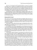
are moderately bullish. The current situation can be seen in Figure 6.1.
The price is currently $115.55 per share. We’d like to buy 100 shares or
the equivalent. So we take a look at the current implied volatility situation
to see if we are bullish or bearish on the implied volatility and therefore
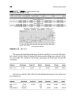
on the options. Figure 6.2 shows the current situation with implied and
historical volatility for IBM. I think that this situation would suggest that
we should be on the short side of options.
We now have decided on the two most important factors affecting op-
tions prices. We want to be long the stock and short volatility. We can now
start to construct a strategy.
It is wise to consider that you can end up with a portfolio of options
but that portfolio will much more closely resemble what you are trying to
achieve. Also note that your portfolio will likely be dynamic. You may be
buying and selling different options to constantly fine tune your net posi-
tion in the market. It is also wise to note that a lot of constructing a strategy
is trial and error. Does this or that work? You may find that you are some-
times going down a wrong path and have to start over (see Figure 6.3).