Báo cáo hóa học: " Research Article Burst Format Design for Optimum Joint Estimation of Doppler-Shift and Doppler-Rate in Packet Satellite Communications" ppt

Hindawi Publishing Corporation
EURASIP Journal on Wireless Communications and Networking
Volume 2007, Article ID 29086, 12 pages
doi:10.1155/2007/29086
Research Article
Burst Format Design for Optimum Joint
Estimation of Doppler-Shift and Doppler-Rate
in Packet Satellite Communications
Luca Giugno,
1
Francesca Zanier,
2
and Marco Luise
2
1
Wiser S.r.l.–Wireless Systems Engineering and Research, Via Fiume 23, 57123 Livorno, Italy
2
Dipartimento di Ingegneria dell’Informazione, University of Pisa, Via Caruso 16, 56122 Pisa, Italy
Received 1 September 2006; Accepted 10 February 2007
Recommended by Anton Donner
This paper considers the problem of optimizing the burst format of packet transmission to perform enhanced-accuracy estimation
of Doppler-shift and Doppler-rate of the carrier of the received signal, due to relative motion between the transmitter and the
receiver. Two novel burst formats that minimize the Doppler-shift and the Doppler-rate Cram
´
er-Rao bounds (CRBs) for the joint
estimation of carrier phase/Doppler-shift and of the Doppler-rate are derived, and a data-aided (DA) estimation algorithm suitable
for each optimal burst format is presented. Performance of the newly derived estimators is evaluated by analysis and by simulation,
showing that such algorithms attain their relevant CRBs with very low complexity, so that they can be directly embedded into new-
generation digital modems for satellite communications at low SNR.
Copyright © 2007 Luca Giugno et al. This is an open access article distributed under the Creative Commons Attribution License,
which permits unrestricted use, distr ibution, and reproduction in any medium, provided the original work is properly cited.

1. INTRODUCTION
Packet transmission of digital data is nowadays adopted
in several wireless communications systems such as satel-
lite time-division multiple access (TDMA) and terrestrial
mobile cellular radio. In those scenarios, the received sig-
nal may suffer from significant time-varying Doppler dis-
tortion due to relative motion between the transmitter and
the receiver. This occurs, for instance, in the last-generation
mobile-satellite communication systems based on a con-
stellation of nongeostationary low-earth-orbit (LEO) satel-
lites [1] and in millimeter-wave mobile communications for
traffic control and assistance [2]. In such situations, car-
rier Doppler-shift and Doppler-rate estimation must be per-
formed at the receiver for correct demodulation of the re-
ceived signal.
Anumberofefficient digital signal processing (DSP) al-
gorithms have already been developed for the estimation of
the Doppler-shift affecting the received carrier [3]andafew
algorithms for Doppler-rate estimation are also available in
the open literature [4, 5]. The issue of joint Doppler-shift
and Doppler-rate estimation has been addressed as well, al-
though to a lesser extent [6, 7]. In all the papers above, the
observed signal is either an unmodulated carrier, or con-
tains pilot symbols known at the receiver. The most common
burstformatistheconventionalpreamble-payload arrange-
ment, wherein al l pilots are consecutive and they are placed
at the beginning of the data burst. Other formats are the mi-
damble as in the GSM system [8], wherein the preamble is
moved to the center of the burst, or the so-called pilot sym-
bol assisted modulation (PSAM) paradigm [9], where the

set of pilot symbols is regularly multiplexed with data sym-
bols in a given ratio (the so-called burst overhead). Data-
aided (DA) algorithms, which exploit the information con-
tained in the pilot symbols, are routinely used to attain good
performance with small burst overhead. The recent intro-
duction of efficient channel coding with iterative detection
[10] has also placed new and more stringent requirements
for receiver synchronization on satellite modems. The car-
rier synchronizer is requested to operate at a lower signal-to-
noise ratio (SNR) than it used to be with conventional coding
[11].
Therefore, it makes sense to search for the ultimate ac-
curacy that can be attained by carrier synchronizers. It turns
out that the Cram
´
er-Rao bounds (CRBs) for joint estima-
tions are functions of the location of the reference symbols
in the burst. The issue to find the optimal burst format that
minimizes the frequency CRB has been already addressed in
2 EURASIP Journal on Wireless Communications and Networking
a
b
N/2 N/2
N/3 N/3N/3
M
-2P format-
-3P format-
Preamble Payload Postamble
M + N/2
M/2 M/2

Payload Payload
L
PPP
c
d
N/4 M/3 N/4 N/4M/3 N/4 M/3
-1st 2P subburst- -2nd 2P subburst-
-4P format-
P
Payload Payload Payload
PPP
2M/3+N/2
Payload Payload
L
PP PP
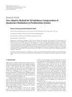
Figure 1: 2P burst format, 3P burst format, and 4P burst format.
[12–14], but only for joint carrier phase/Doppler-shift es-
timation. The novelty of the paper is to extend the anal-
ysis to the joint carrier phase/Doppler-shift and Doppler-
rate estimation. It is known [12–15] that the preamble-
postamble format (2P format) described in the sequel min-
imizes the frequency CRB with no Doppler-rate, and with
constraints on the total training block length and on the
burst overhead of the signal. We demonstrate here that such
format is optimal in the presence of Doppler-rate as well,
and that the Doppler-rate CRB is minimized by estima-
tion over three equal-length blocks of reference symbols that
are equally spaced by data symbols (3P format). We also
show that other formats are very close to optimality (4P for-
mat).

In addition to computation of the burst, we also in-
troduce new high-resolution and low-complexity carrier
Doppler-shift and Doppler-rate DA estimation algorithms
for such optimal burst formats.
The paper is organized as follows. In Section 2,we
first outline the received signal model affected by Doppler
distortions. Next, in Section 3 we present and analyze a
low-complexity DA Doppler-shift estimator for the optimal
2P format. Extensions of this algorithm for joint carrier
phase/Doppler-shift and Doppler-rate estimation for the 2P
format, the 3P format, and the sub-optimum 4P format, are
introduced in Sections 4 and 5, respectively. Finally, some
conclusions are drawn in Section 6.
2. SIGNAL MODEL
In this paper, we take into consideration three different data
burst formats as depicted in Figure 1.
In all cases, the total number of pilot symbols that are
known to the receiver is equal to N, and the total length of
the “data payload” fields that contain information symbols is
equal to M. The formats differ for the specific pilots arrange-
ment in two/three/four groups of N/2, N/3, N/4consecutive
pilot symbols equally spaced by data symbols. Hereafter we
will address them as “2P,” “ 3P,” “ 4P” formats as in Figures
1(a), 1(b), 1(c), respectively. We denote also with L
= N + M
the overall burst length, and with η the burst overhead, that
is, the ratio between the total number of pilot symbols and
the total number of symbols within the burst:
η
=

N
L
=
N
N + M
=
1
1+M/N
. (1)
We also assume BPSK/QPSK data modulation for the pilot
fields, and additive white Gaussian noise (AWGN) channel
with no multipath. Filtering is evenly split between transmit-
ter and receiver, and the overall channel response is Nyquist.
Timing recovery is ideal but the received signal is affected by
time-varying Doppler distortion. Filtering the received wave-
form with a matched filter and sampling at symbol rate at
the zero intersymbol interference instants yields the follow-
ing discrete-time signal:
z(k)
= c
k
e
jϕ
k
+ n(k), k =−
L − 1
2
, ,0, ,
L
− 1

2
,
(2)
where
ϕ
k
= θ +2πνkT + παk
2
T
2
(3)
is the instantaneous carrier excess phase,
{c
k
} are unit-energy
(QPSK) data symbols and L (odd) is the observation (burst)
length. Also, 1/T is the symbol rate, θ is the unknown initial
carrier phase, ν is the constant unknown carrier frequency
offset (Doppler-shift), and finally α is the constant unknown
carrier frequency rate-of-change (Doppler-rate). For signal
model (2) to be valid, we assumed that the value of the
Doppler-shift ν is much smaller than the symbol rate, and
that the value of the Doppler-rate α is much smaller than
the square of the symbol rate. The noise n(k) is a complex-
valued zero-mean WGN process with independent compo-
nents, each with variance σ
2
= N
0
/(2E

s
), where E
s
/N
0
repre-
sents the ratio between the received energy-per-symbol and
the one-sided channel noise power spectral density.
Estimation of ν and α from the received signal z(k)re-
quires preliminary modulation removal from the pilot fields.
Broadly speaking, it is customary to adopt BPSK or QPSK
modulation for pilot fields, so that modulation removal is
easily carried out by letting r(k)
= c
∗
k
z(k). The result is
r(k)
= e
jϕ
k
+ w(k), k ∈ K =


N
P
i

,(4)
Luca Giugno et al. 3

where K is the symmetric set of N time indices correspond-
ing to pilot symbols, and w(k)
= c
∗
k
n(k) is statistically equiv-
alent to n(k). We explicitly mention here that we have cho-
sen a symmetrical range K with respect to the middle of
the burst since such arrangement decouples the estimation
of some parameters, as discussed in [12] and in Appendix B.
The signal r(k)willbeconsideredfromnowonasourob-
served signal that allows to carry out the carrier synchro-
nization functions. We show in Appendix B that the burst
formats in Figure 1 are optimum so far as the estimation of
parameters ν and α is concerned. To keep complexity low, we
will not take into consideration here “mixed,” partially blind,
methods to perfor m carrier synchronization that use both the
known pilot symbols and all of the intermediate data sym-
bols of the burst, like envisaged in [16] for the case of channel
estimation.
3. DOPPLER-SHIFT ESTIMATOR: FEPE ALGORITHM
We momentarily neglect the effect of the Doppler-rate α in
(4), to concentrate on the issue of Doppler-shift estimation
only. Under such hypothesis, (4) can be rewritten as follows:
r(k)
= e
j(θ+2πνkT)
+ w(k), k ∈ K. (5)
The 2P format minimizes the CRB for Doppler-shift esti-
mation for joint carrier phase/Doppler-shift estimation [12–

15]. Conventional frequency offset estimators for consecu-
tive signal samples [3] are not directly applicable to a burst
format encompassing a preamble and a postamble. In addi-
tion, straightforward solution of a maximum-likelihood es-
timation problem for ν appears infeasible. We introduce thus
a new low-complexity algorithm suitable for the estimation
of the Doppler-shift ν in (4) with the burst format as above.
The key idea of the 2P frequency estimator is really a naive
one: we start by computing two phase estimates, the one on
the preamble section, and the other on the postamble, us-
ing the standard low-complexity maximum-likelihood (ML)
algorithm [17]:

θ
1
=arg

−(M−1)/2

k=−(N+M−1)/2
r(k)

,

θ
2
=arg

(N+M−1)/2


k=(M−1)/2
r(k)

,
(6)
where arg
{·} denotes the phase of the complex-valued ar-
gument. Then we associate the two phase estimates to the
two midpoints of the preamble and postamble sections, re-
spectively, whose time distance is equal to (M + N/2)T
(Figure 1(a)). After this is done, we simply derive the fre-
quency estimate as the slope of the line that connects the two
points (
−(M − 1)/2 − N/4,

θ
1
)and((M − 1)/2+N/4,

θ
2
)on
the (time, phase) plane:
ν =





θ

2


2π
−



θ
1


2π


2π
2π(M + N/2)T
. (7)
This simple algorithm is known as frequency estimation
through phase estimation (FEPE) [15]. The operator
|x|
2π
re-
turns the value of x modulo 2π, in order to avoid phase am-
biguities, and is trivial to implement when operating with
−1.5
−1
−0.5
0
0.5

1
1.5
×10
−3
MEV
−1.5 −1 −0.50 0.511.5
×10
−3
νT (Hz × s)
Ideal
E
s
/N
0
= 0dB
E
s
/N
0
= 10 dB
E
s
/N
0
= 20 dB
E
s
/N
0
= 100 dB

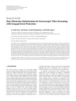
Figure 2:MEVofFEPEestimatorfordifferent values of E
S
/N
0
—
simulation only. Preamble + postamble DA ML phase estimation,
N
= 44, M = 385.
fixed-point arithmetic on a digital hardware. It is easy to ver-
ify that such estimator is independent of the particular ini-
tial phase θ, that vanishes when computing the phase dif-
ference at the numerator of (7). It is also clear that the
operating range of the estimator is quite narrow. In order
not to have estimation ambiguities, we have to ensure that
−π ≤|

θ
2
|
2π
−|

θ
1
|
2π
<π, and therefore the range is bounded
to
|ν|≤
1

2(M + N/2)T
. (8)
This relatively narrow interval does not allow to use the FEPE
algorithm for initial acquisition of a large frequency offset at
receiver start-up. Its use is therefore restricted to fine esti-
mation of a residual offset after a coarse acquisition or com-
pensation of motion-induced Doppler-shift. Figure 2 depicts
the normalized mean estimated value (MEV) curves of the
FEPE algorithm (i.e., the average estimated value E
{ν} as a
function of the true Doppler-shift ν)fordifferent values of
E
s
/N
0
as derived by simulation. In our simulations we use
the values N
= 44 and M = 385 taken from the design de-
scribedin[11], so that the overhead is η
= 10% (typical for
short bursts). MEV curves show that the algorithm is unbi-
ased in a broad range around the true value (here, ν
= 0). It
can be shown that this is true as long as ν2NT
 1, so that
the “ancillary” estimates

θ
2
and


θ
1
are substantially unbiased
as well. Such condition is implicitly assumed in (8) since in
the practice M
 N/2. The curve labeled E
s
/N
0
= 100 dB
(which is totally unrealistic) has the only purpose of showing
the bounds of the unambiguous estimation range.
It is also easy to evaluate the estimation error variance of
the FEPE estimator. It is known in fact that

θ
1
and

θ
2
in (7)
have an estimation variance σ
2

θ
that achieves the Cram
´
er-Rao

4 EURASIP Journal on Wireless Communications and Networking
Bound (CRB)[17]:
σ
2

θ
= CRB(θ) =
1
2 · N/2
1
E
s
/N
0
. (9)
Therefore, considering that the two phase estimates i n (7)are
independent, we get
σ
2
FEPE
(ν)=
2 · σ
2

θ
4π
2
(M + N/2)
2
T

2
=
1
4π
2
T
2
N/2(M + N/2)
2
1
E
s
/N
0
.
(10)
The vector CRB [18] for the frequency offset estimate in the
joint carrier phase/Doppler-shift estimation with the 2P for-
mat is derived in Appendix A and reads as follows:
VCRB
2P
(ν)=
3
4π
2
T
2
(N/2)

4(N/2)

2
+3M
2
+3MN−1

1
E
s
/N
0
.
(11)
Both from the expression of the bound (11) and of the
variance (10), it is seen that the estimation accuracy has an
inverse dependence on (N/2)
3
, and this is nothing new with
respect to conventional estimation on a preamble only. The
important thing is that we also have inverse dependence on
M
2
, due to the 2P format that gives enhanced accuracy (with
small estimation complexity) with respect to the conven-
tional estimator. From (1), we also have M
= N(1/η − 1),
so that the term 3M
2
dominates (N/2)
2
as long as η<1/2,

which is always verified in the practice.
Therefore, the ratio between the CRB (11) and the vari-
ance of the FEPE estimator is very close to 1. With N
= 44
and M
= 385, we get, for instance, σ
2
FEPE
/VCRB
2p
= 0.99.
The enhanced-accuracy feature is also apparent in the com-
parison of the VCRB
2p
(ν)asin(11) with the conventional
VCRB(ν)[18] for frequency estimation on a single preamble
with length N, that is obtained by letting M
= 0in(11). The
reverse of the coin is of course the reduced operating range
(8) of the estimator.
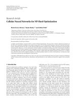
Figure 3 shows curves of the (symbol-rate-normalized)
RMSEE (root mean square estimation error) of the FEPE
algorithm (i.e., T

E{(v − v)
2
}) as a function of E
s
/N
0

for
various values of the true offset ν.Inparticular,marksare
simulation results for σ
2
FEPE
, whilst the lowermost line is the
VCRB
2p
(ν). We do not report the curve for (10) since it
would be totally overlapped with (11).
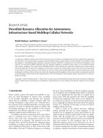
Performance assessment of the FEPE estimator is con-
cluded in Figure 4 with the evaluation of the sensitivity of the
RMSEE to different values of an uncompensated Doppler-
rate α.JusttohaveanideaofpracticalvaluesofαT
2
to be en-
countered in practice, we mention that the largest Doppler-
rates in LEO satellites are of the order of 200 Hz/s [1, 19]for
a carrier frequency of 2.2 GHz, and assuming a symbol rate
of 2 Mbaud, we end up with the value αT
2
= 5.10
−11
.From
simulation results, we highlight that the performance of this
algorithm is affected by α, but only in the case of a normal-
ized Doppler-rate αT
2
≥ 10
−7

, that is larger than those that
are found in the practice.
Finally, the complexity of the FEPE estimator with re-
spect to conventional methods of frequency estimation [3,
10
−6
10
−5
10
−4
10
−3
10
−2
Normalized RMSEE
0 1 2 3 4 5 6 7 8 9 10 11 12 13 14 15 16 17 18 19 20
E
s
/N
0
(dB)
σ
2
FEPE
(ν)
νT
= 1 × 10
−3
νT = 1 × 10
−4

VCRB (ν)
VCRB
2P
(ν)
Figure 3: RMSEE of FEPE estimator for different values of
E
S
/N
0
and relevant bounds—solid lines: theory—marks: simula-
tion. Preamble + postamble DA ML phase estimation, N
= 44,
M
= 385.
13] is presented in Table 1. It is clear that the strength of the
FEPE algorithm is its very low complexity as compared to
conventional algorithms.
4. DOPPLER-RATE ESTIMATORS IN 2P FRAME:
FREPE AND FREFE ALGORITHMS
We take now back into consideration the presence of a non-
negligible Doppler-rate in the received signal, modeled as in
(3)-(4). We focus again on the 2P format (Figure 1(a)), since
it is the optimal format for Doppler-shift estimation in joint
carrier phase/Doppler-shift and Doppler-rate estimation too,
as demonstrated in Appendix B. A new simple estimator for
α in the 2P format is found by a straightforward general-
ization of the FEPE approach. Assume that we further split
both the preamble and the postamble into two subsections of
equal length, and we compute four (independent) ML phase
estimates on the two subsections. We know in advance that

the time evolution of the phase is described by a parabola.
The four phase estimates can thus be used to fit a second-
order phase polynomial according to the Minimum Mean
Squared Error (MMSE) criterion; taking the origin in the
Luca Giugno et al. 5
10
−6
2
3
4
5
6
7
10
−5
2
3
4
5
6
7
10
−4
2
3
4
5
6
7
10

−3
Normalized RMSEE
0 1 2 3 4 5 6 7 8 9 10 11 12 13 14 15 16 17 18 19 20
E
s
/N
0
(dB)
VCRB
2P
(ν)
αT
2
= 0
αT
2
= 2 × 10
−8
αT
2
= 5 × 10
−8
αT
2
= 1 × 10
−7
αT
2
= 2 × 10
−7

αT
2
= 2.5 × 10
−7
Figure 4: Sensitivity of FEPE estimator to different values of the
Doppler-rate αT
2
. Preamble + postamble DA ML phase estimation,
N
= 44, M = 385, vT = 1.0 × 10
−3
.
first section of the preamble, we obtain the phase model
ϕ
P
(n) = aπ

n +
M
− 1
2
+
3N
8

2
+2πb

n +
M

− 1
2
+
3N
8

+ c,
(12)
where the regression coefficients a and b directly repre-
sent estimates for the (normalized) carrier Doppler-rate and
Doppler-shift, respectively, and c is an estimate for the initial
phase (that we are not interested into). The coefficients are
found after observing that the MSE is written as
ε(a, b, c)
=
4

i=1

ϕ
P

n
i

−

θ
i


2
=
4

i=1
e
2
i
, (13)
where

θ
i
, i = 1, , 4, are the above-mentioned ML phase
estimates on N/4 pilots each, and n
1
=−[(M − 1)/2+3N/8],
n
2
=−[(M − 1)/2+N/8], n
3
= [(M − 1)/2+N/8], and
n
4
= [(M − 1)/2+3N/8] are the four time instants that we
conventionally associate to the four estimates (the midpoints
of the four subsections). Equating to zero the derivatives of
Table 1: The FEPE computational complexity comparison.
(N
alg

= estimation design parameter.)
Computational complexity of major
Doppler-shift estimation algorithms
Algorithm Reference
Number of real products
and additions
LUT access
L&R [3] 4N

N
alg
+1

−
2 1
M&M [3]
N
alg

8N − 4N
alg
− 3

−
2 N
alg
S-BLUE [13] 4N
2
+4.5N − 3 1.5N − 2
P-BLUE-2 [13]

4N − 1 1
FEPE —
2N +3 2
ε(a, b, c)withrespecttoa, b,andc,weobtain
∂ε(a, b, c)
∂a
=
4

i=1
e
i
·

n
i
+

M − 1
2
+
3N
8

2
= 0,
∂ε(a, b, c)
∂b
=
4


i=1
e
i
·

n
i
+

M − 1
2
+
3N
8

=
0,
∂ε(a, b, c)
∂c
=
4

i=1
e
i
= 0,
(14)
and solving for a we get the following so-called frequency rate
estimation through phase estimation (FREPE) algorithm [15]:

α
FREPE
=
a
T
2
=


θ
4
−

θ
3

−


θ
2
−

θ
1

πN/2(N/2+M)T
2
(15)
(all differences to be intended m odulo-2π). This extremely

simple approach can be viewed as a generalization of the
FEPE introduced in the previous section. In particular, by us-
ing (7), the terms


θ
i
−

θ
i−1

2π(N/4)T
, i
= 2, 4, (16)
represent two Doppler-shift estimations, the first on the
preamble and the second on the postamble, respectively,
which are spaced M + N/2 symbols apart. The Doppler-rate
estimate is thus simply the difference between the two fre-
quency estimates, divided by their time distance (M +N/2)T.
The considerations above allow us to also introduce
the frequency rate estimation through frequency estimation
(FREFE) algorithm [15]
α
FREFE
=

ν
2
− ν

1
(M + N/2)T
, (17)
wherein the two frequency estimates
ν
1
and ν
2
can be ob-
tained by any conventional algorithm [3] operating sepa-
rately on the preamble and on the postamble, respectively.
We can choose for instance the L&R algorithm [20] or the
R&B algorithm [21]. Assuming that the selected algorithm
operates close enough to the CRB (as is shown in [3]), the
6 EURASIP Journal on Wireless Communications and Networking
variance of (17)is
σ
2
FREFE
(α) =
2σ
2
ν
(M + N/2)
2
T
2
=
3
π

2
T
4
N/2

(N/2)
2
− 1

(M + N/2)
2
1
E
s
/N
0
,
(18)
wherewehaveusedσ
2
ν
= 3 · (E
s
/N
0
)
−1
/[2π
2
T

2
N/2((N/2)
2
−
1)] [17]. This can be compared to the variance of the FREPE
algorithm that is easily found to be
σ
2
FREPE
(α) =
4 · σ
2

θ
π
2
(N/2)
2
(M + N/2)
2
T
4
=
4
π
2
T
4
(N/2)
3

(M + N/2)
2
1
E
s
/N
0
,
(19)
where now σ
2

θ
= (E
s
/N
0
)
−1
/(N/2). The relevant vector CRB
for Doppler-rate estimate is (see Appendix B):
VCRB
2P
(α)
=
45
π
2
T
4


(N/2)
3
−N/2

16(N/2)
2
+15 M
2
+30MN/2−4

1
E
s
/N
0
.
(20)
All expressions inversely depend on (N/2)
5
as in conven-
tional preamble-only estimation of the Doppler-rate [6], but
they also bear again inverse dependence on M
2
that gives en-
hanced accuracy. For sufficiently large values of N and M,
M
 N,wehave
σ
2

FREFE
(α)
σ
2
FREPE
(α)
∼
=
3
4
,
VCRB
PP
(α)
σ
2
FREFE
(α)
∼
=
1. (21)
Figure 5 shows the MEV curves (i.e., E
{α}) of the FREPE al-
gorithm for different values of E
s
/N
0
, in the case of N = 44,
M
= 385, and Doppler-shift vT = 10

−3
. The estimator is
unbiased with an operating range equal to


α
FREPE


≤
1
N/2(M + N/2)T
2
. (22)
The sensitivity of FREPE to different uncompensated val-
ues of vT is illustrated in Figure 6 in terms of MEV.
The same simulations have been run also for the FREFE
algorithm. In particular, Figure 7 illustrates the MEV curves
for different values of E
s
/N
0
and with vT = 10
−3
. By u sing
the L&R a lgorithm to estimate
ν
1
and ν
2

, the operating range
of FREFE is roughly twice that of FREPE:


α
FREFE


≤
1
(N/4+1)(M + N/2)T
2
. (23)
In particular, the term [(N/2+1)T]
−1
represents the fre-
quency pull-in range of L&R on N/2 pilots [20].
Figure 8 demonstrates that FREPE is also less sensitive
than FREFE to an uncompensated Doppler-shift. Finally,
Figure 9 shows the curve of the Doppler-rate RMSEE of
FREPE and FREFE as a function of E
s
/N
0
,forνT = 10
−3
and
αT
2
= 10

−6
. The FREPE estimator loses only 10 log
10
(4/3) =
1.25 dB in terms of E
s
/N
0
with respect to the performance of
the more complex FREFE when N
 1.
−1.5
−1
−0.5
0
0.5
1
1.5
×10
−4
MEV
−1.5 −1 −0.50 0.5
1
1.5
×10
−4
αT
2
(Hz/s × s
2

)
Ideal
E
s
/N
0
= 0dB
E
s
/N
0
= 10 dB
E
s
/N
0
= 20 dB
E
s
/N
0
= 100 dB
Figure 5: MEV of FREPE estimator for different values of E
S
/N
0
—
simulation only. Preamble + postamble DA ML phase estimation,
N
= 44, M = 385, vT = 1.0 × 10

−3
.
−1.5
−1
−0.5
0
0.5
1
1.5
×10
−4
MEV
−1.5 −1 −0.50 0.511.5
×10
−4
αT
2
(Hz/s × s
2
)
Ideal
νT
= 0
νT
= 1 × 10
−3
νT = 5 × 10
−3
νT = 1 × 10
−2

Figure 6: MEV of FREPE estimator for differ ent values of the
Doppler-shift vT—simulation only. Preamble + postamble DA ML
phase estimation, N
= 44, M = 385, E
s
/N
0
= 10 dB.
5. OPTIMUM DOPPLER-RATE ESTIMATION
5.1. Odd number of pilot fields: FRE-3PE algorithm
We turn now to the issue of optimum burst configuration
for the estimation of the Doppler-rate. We demonstrate in
Appendix B that the 3P format (Figure 1(b)) minimizes the
CRB for Doppler-rate estimation, with the usual constraints
on the total training block length and on the burst over-
head (1). In the following, we develop a new low-complexity
algorithm suitable for Doppler-rate estimation with the 3P
format. We know in advance that the time evolution of the
phase is described by a parabola. As was done for the FREPE
Luca Giugno et al. 7
−2.5
−2
−1.5
−1
−0.5
0
0.5
1
1.5
2

2.5
×10
−4
MEV
−2.5 −2 −1.5 −1 −0.50 0.51 1.522.5
×10
−4
αT
2
(Hz/s × s
2
)
Ideal
E
s
/N
0
= 0dB
E
s
/N
0
= 10 dB
E
s
/N
0
= 20 dB
E
s

/N
0
= 100 dB
Figure 7: MEV of FREFE estimator for different values of E
S
/N
0
—
simulation only. Preamble + postamble Luise and Reggiannini, N
=
44, M = 385, vT = 1.0 × 10
−3
.
−2.5
−2
−1.5
−1
−0.5
0
0.5
1
1.5
2
2.5
×10
−4
MEV
−2.5 −2 −1.5 −1 −0.50 0.51 1.522.5
×10
−4

αT
2
(Hz/s × s
2
)
Ideal
νT
= 0
νT
= 1 × 10
−3
νT = 5 × 10
−3
νT = 1 × 10
−2
Figure 8: MEV of FREFE estimator for different values of the
Doppler-shift vT—simulation only. FREFE estimator preamble +
postamble Luise and Reggiannini, N
= 44, M = 385, E
s
/N
0
=
10 dB.
algorithm in the 2P configuration, a simple estimator of α
in the 3P format is found by computing three (independent)
ML phase estimates on the three blocks of pilots, and then
fitting a second-order phase polynomial. Taking the origin in
the first block of pilots, we obtain this time the phase model
ϕ

P
(n) = aπ

n +
N
3
+
M
2

2
+2πb

n +
N
3
+
M
2

+ c. (24)
The coefficients are found solving the following set of equa-
tions:
ϕ
P

n
i

=


θ
i
, i = 1, , 3, (25)
10
−8
10
−7
10
−6
10
−5
10
−4
10
−3
Normalized RMSEE
0 1 2 3 4 5 6 7 8 9 10 11 12 13 14 15 16 17 18 19 20
E
s
/N
0
(dB)
FREPE, αT
2
= 1 × 10
−6
FREFE, αT
2
= 1 × 10

−6
FRE-2FEPE, αT
2
= 1 × 10
−6
FRE-3PE, αT
2
= 1 × 10
−6
VCRB
P
(α)
VCRB
2P
(α)
VCRB
4P
(α)
VCRB
3P
(α)
Figure 9: RMSEE of FREPE, FREFE, FRE-3PE, and FRE-2FREPE
estimators for different values of E
S
/N
0
and relevant bounds,—solid
lines: theory—marks: simulation. Doppler-rate algorithms: FREFE
versus FREPE versus FRE-3PE versus FRE-2FEPE, N
= 44(45),

M
= 385(384), vT = 1.0 × 10
−3
.
where

θ
i
are the above-mentioned ML phase estimates on
N/3 pilots each, and where n
1
=−(M/2+N/3), n
2
= 0, and
n
3
= (M/2+N/3) are the three time instants that we con-
ventionally associate to the three estimates (the midpoints of
the three subsections). Solving for a, we get the following so-
called (FRE-3PE) (frequency rate estimation throug h 3 phase
estimations) algorithm:
α
FRE-3PE
=
a
T
2
=
18



θ
3
−

θ
2

−


θ
2
−

θ
1

π(2N +3M − 2)
2
T
2
(26)
(all differences to be intended modulo-2π). The estimator is
unbiased with an operating range equal to:



α
FRE-3PE



≤
18
(2N +3M − 2)
2
T
2
. (27)
In our simulations (N
= 45 and M = 384), |α
FRE-3PE
· T
2
|≤
10
−5
. This range is narrower than FREPE’s and FREFE’s in
the 2P format, but it still widely includes practical Doppler-
rate values mentioned in Section 3. Figure 10 shows the MEV
curves of the FRE-3PE algorithm for different values of
E
s
/N
0
, in the case of N = 45, M = 384, and Doppler-shift
8 EURASIP Journal on Wireless Communications and Networking
−1.5
−1
−0.5

0
0.5
1
1.5
×10
−5
MEV
−1.5 −1 −0.50 0.51 1.5
×10
−5
αT
2
(Hz/s × s
2
)
Ideal
E
s
/N
0
= 0dB
E
s
/N
0
= 10 dB
E
s
/N
0

= 20 dB
E
s
/N
0
= 100 dB
Figure 10: MEV of FRE-3PE estimator for di fferent values of
E
S
/N
0
—simulation only. 3 blocks of pilots DA ML phase estima-
tion, N
= 45, M = 384, vT = 1.0 × 10
−3
.
vT = 10
−4
, while Figure 11 shows the sensitivity of the MEV
to different u ncompensated values of the Doppler-shift vT.
The theoretical error variance of the FRE-3PE estimator
can be easily evaluated, similarly to what was done for the
calculation of σ
2
FREFE
(α)inSection 4:
σ
2
FRE-3PE
(α) =

18
2
· 6 · σ
2

θ
π
2
(2N +3M − 2)
4
T
4
=
18
2
· 6
π
2
T
4
(2N/3)(2N +3M − 2)
4
1
E
s
/N
0
,
(28)
where now σ

2

θ
= (E
s
/N
0
)
−1
/(2N/3). Comparing this expres-
sion wi th the VCRB
3P
(α)in(B.11) and with the variances of
the FREFE and FREPE algorithms, we note that all expres-
sions inversely depend on N
5
as in conventional preamble-
only estimation of the Doppler-rate [6]. On the other hand,
σ
2
FRE-3PE
(α)andVCRB
3P
(α)inverselydependonM
4
,out-
performing the accuracy of both the traditional preamble-
only format and the 2P format (that depends on M
−2
). The

enhanced accuracy is highlighted by Figure 9, where we re-
port the simulated RMSEE (marks) of FRE-3PE, FREPE, and
FREFE versus E
s
/N
0
. To perform a fair comparison, we also
reported the VCRB
P
(β), obtained in the case of estimation of
Doppler-rate in the preamble-only configuration. The FRE-
3PE algorithm attains its own CRB, and exhibits a gain of
19 dB in terms of E
s
/N
0
with respect to the 2P format.
As a final remark, we only mention that a simple estima-
tor of Doppler-shift in the 3P format is found by applying the
FEPE algorithm to the two extreme pilot fields of the burst.
Its variance reaches the VCRB
3P
(ν) calculated setting x = 1
in (B.7)and(B.9), that is 1.5 dB apart from the VCRB
2P
(ν)
of the optimal 2P format.
−1.5
−1
−0.5

0
0.5
1
1.5
×10
−5
MEV
−1.5 −1 −0.50 0.51 1.5
×10
−5
αT
2
(Hz/s × s
2
)
Ideal
νT
= 0
νT
= 1 × 10
−4
νT = 5 × 10
−4
νT = 1 × 10
−3
Figure 11: MEV of FRE-3PE estimator for different values of the
Doppler-shift vT—simulation only. 3 blocks of pilots, N
= 45, M =
384, E
S

/N
0
= 10 dB.
5.2. Even number of pilot fields: FRE-2FEPE algorithm
When the number of pilot fields is even, the optimum burst
format turns out to be the 4P as shown in Appendix B.
We notice that the ratio of the two bounds for 3P and
4P amounts to VCRB
4p
(α)/VCRB
3p
(α)
∼
=
9720/108 · 640/
51840
∼
=
1.09 M  N, so that 4P is only slightly optimal.
A simple estimator of α in the 4P format is found by a
straightforward generalization of the FEPE and FREFE ap-
proaches. Assume that we split the burst into two 2P sub-
bursts of length (M/3+N/2), (Figure 1(d)). Each preamble
and postamble is now of length N/4, and we can derive two
FEPE estimates of frequency on each subburst:
ν
1
=






θ
2


2π
−



θ
1


2π


2π
2π(M/3+N/4)T
,
ν
2
=






θ
4


2π
−



θ
3


2π


2π
2π(M/3+N/4)T
,
(29)
where

θ
i
, i = 1, , 4, are the ML phase estimates computed
on the four pilot fields of N/4 pilots each. The two Doppler-
shift estimates
ν
1
and ν

2
are associated with the two mid-
point instants of the two 2P subbursts, whose time distance
is equal to (2M/3+N/2)T (Figure 1(c)). Again, we estimate
the Doppler-rate as the slope of the line that connects the two
points (
−(M/3 − 1/2) − N/4, ν
1
)and((M/3 − 1/2) + N/4, ν
2
)
in the (time, frequency) plane:
α
FRE-2FEPE
=

ν
2
− ν
1
(2M/3+N/2)T
. (30)
We call this algorithm FRE-2FEPE (frequency rate estimation
through two FEPE estimations).
It is clear that the operating range of the estimator with
respect to
ν comes from the application of (8) to the new
configuration and turns out to be
|ν|≤[2(M/3+N/4)T]
−1

.
The M EV curves of FRE-2FEPE are not reported here since
Luca Giugno et al. 9
they basically mimic those in Figures 10 and 11 for the
FRE-3PE algorithm. The estimation error variance of (30)
is found to b e
σ
2
FRE-2FEPE
(α) =
σ
2

θ
(2M/3+N/2)
2
(M/3+N/4)
2
π
2
T
2
=
2 ·

E
s
/N
0


−1
π
2
T
4
N(2M/3+N/2)
2
(M/3+N/4)
2
.
(31)
Figure 9 shows also the curves of the RMSEE of FRE-2FEPE
and its respective CRB. The FRE-2FEPE algorithm reaches its
own V CRB
4p
(α) and thus, as demonstrated in Appendix B,it
gains 10 log
10
(7.19) = 18.5dBintermsofE
s
/N
0
with respect
to the performance of the previous algorithms with the 2P
format. Also, the FRE-2FEPE loses only 0.4 dB with respect
to the FRE-3PE algorithm and can thus be a valid alternative
to the 3P format.
As a final remark, we briefly address the issue of Doppler-
shift estimation in the 4P format. The best method is found
by applying the FEPE algorithm to the two extreme pilot

fields of the burst. Its variance is close to the VCRB
4P
(ν)cal-
culated setting x
= 1in(B.8)and(B.9), that is 2.4 dB worse
than the VCRB
2P
(ν) of the optimal 2P format.
6. CONCLUSIONS
In this paper, we presented and analyzed some very-
low-complexity algorithms for carrier Doppler-shift and
Doppler-rate estimation in burst digital transmission. To
achieve enhanced accuracy, the burst configurations that
minimize the CRB for the estimation of Doppler-shift and
Doppler-rate are derived. O ur analysis showed that the 2P
format is optimum for Doppler-shift estimation and that the
3P format is optimum for Doppler-rate estimation. These
two configurations can be practically thought as repetition of
two/three consecutive conventional (preamble-only) bursts.
Despite preventing from real-time processing of the data pay-
load section, the 2P and 3P formats greatly outperform the
estimation based on conventional preamble-only pilot dis-
tribution. Performance assessment has shown that all of the
proposed algorithms are unbiased in practical operating con-
ditions, and that their accuracy in terms of estimation vari-
ance gets remarkably close to their respective CRBsdownto
very low E
s
/N
0

values.
APPENDICES
A. VCRB FOR JOINT CARRIER PHASE/DOPPLER-SHIFT
ESTIMATION WITH 2P FORMAT
In this appendix, we calculate the VCRB for the error vari-
ance of any unbiased estimator of Doppler-shift in the case of
joint estimation of phase/Doppler-shift using the preamble-
postamble (2P) format. We explicitly mention that we have
chosen a set K of pilot locations that is symmetr ical with
respect to the middle of the burst, since a symmetrical K de-
couples phase from Doppler-shift estimation, as discussed in
[12]. After modulation removal, the generic sample within
the preamble and the postamble is given by (5).
The Fisher information matrix (FIM) [18]canbewritten
as
F
=

F
θθ
F
θν
F
νθ
F
νν

=
⎡
⎢

⎢
⎢
⎢
⎣
−
E
r






∂
2
ln p(r | ν,

θ)
∂

θ
2






−
E

r






∂
2
ln p(r | ν,

θ)
∂

θ∂ν






−
E
r







∂
2
ln p(r | ν,

θ)
∂ν∂

θ






−
E
r






∂
2
ln p(r | ν,

θ)
∂ν
2







⎤
⎥
⎥
⎥
⎥
⎦
,
(A.1)
where p(r
| ν,

θ) is the probability density function of r =
{
r(k)}, k ∈ K, conditioned on (ν,

θ), and r(k)isarandom
Gaussian variable with variance equal to σ
2
= N
0
/(2E
s
)and
mean value equal to

s(k) = e
j(

θ+2πνkT)
. (A.2)
Therefore, we write p(r
| ν,

θ)as
p(r
| ν,

θ) =

k∈K
p

r
k
| ν,

θ

=
1

2πσ
2

N

exp

−
1
2σ
2

k∈K


r(k) − s(k)


2

.
(A.3)
Taking the logarithm of (A.3), we obtain
ln p(r
| ν,

θ)
= N ln

1
2πσ
2

−
1

2σ
2

k∈K



r(k)


2
+



s(k)


2
− 2Re

r(k)s
∗
(k)

=
C +
1
σ
2


k∈K
Re

r(k)s
∗
(k)

,
(A.4)
where C is a constant term that includes all the quantities
independent of
ν and

θ.Afterdifferentiating twice (A.4)with
respect to
ν and

θ, calculating the expectation of the various
terms with respect to r,weget
F
=

a

b

c

d



,(A.5)
where
a

=

1
σ
2


k∈K

(1)E
r

Re

r(k)s
∗
(k)

,
b

=

1

σ
2


k∈K

(2πTk)E
r

Re

r(k)s
∗
(k)

,
c

=

1
σ
2


k∈K

(2πTk)E
r


Re

r(k)s
∗
(k)

,
d

=

1
σ
2


k∈K

4π
2
T
2
k
2

E
r

Re


r(k)s
∗
(k)

.
(A.6)
10 EURASIP Journal on Wireless Communications and Networking
By noticing that
E
r

Re

r(k)s
∗
(k)

=
1, (A.7)
we obtain
F =
1
σ
2
⎡
⎢
⎢
⎢
⎢
⎣


k∈K
(1) 2πT

k∈K
k
2πT

k∈K
k 4π
2
T
2

k∈K
k
2
⎤
⎥
⎥
⎥
⎥
⎦
,(A.8)
where, considering the symmetry of the range K ,

k∈K
(1) = N,

k∈K

k = 0, (A.9)

k∈K
k
2
=
N/2
3

8

N
2

2
− 6

N
2

+1
+3M
2
+3M

3

N
2


−
1

.
(A.10)
After calculation of F
−1
, the VCRB for ν in case of joint
phase/Doppler-shift estimation is found to be
F
−1
νν
= VCRB
2P
(ν) =
1
2π
2
T
2

k∈K
k
2
1
E
s
/N
0
=

3 ·

E
s
/N
0

−1
4π
2
T
2
(N/2)

4(N/2)
2
+3M
2
+3MN − 1

.
(A.11)
B. OPTIMAL SYMMETRIC BURST CONFIGURATION
FOR JOINT CARRIER-PHASE/DOPPLER-SHIFT
AND DOPPLER-RATE ESTIMATION:
2P, 3P, 4P FORMATS
This appendix addresses the optimal signal design for
Doppler-shift ν and Doppler-rate α estimation in the case of
joint phase/Doppler-shift and Doppler-rate estimation when
the received signal is expressed by (2)–(4). The optimal train-

ing signal structure is developed by minimizing the vector
Cram
´
er-Rao bounds (VCRBs) [17, 18]forν and α,with
constraints on the total training block length and on the
burst overhead (1) of the sig nal (4). In fact, the Cram
´
er-Rao
bounds (CRBs) for joint estimations are functions of the lo-
cation of the reference symbols in the burst.
The issue of finding the optimal burst format that mini-
mizes the frequency CRB has been already addressed in [12–
14], but only for joint phase/Doppler-shift estimation. We
restrict our analysis to a symmetric burst format. In the se-
quel, we demonstrate that this symmetry also decouples the
estimation of Doppler-shift and Doppler-rate. Our attention
is focused on a generic burst format as in Figure 12, either
with an even (Figure 12(a))oranodd(Figure 12(b))num-
ber of blocks of pilots. Just to rehearse notation, we mention
that the length of the burst is L symbols, N is the total num-
ber of pilot symbols, N
P
is the number of reference symbols
in each subgroup, M is the total number of data symbols,
and M
D
is the number of data symbols in each subgroup.
In Figure 12(a),2x
even
is the (even) number of subgroups of

N
P
M
D
N
P
M
D
N
P
M
D
N
P
M
D
N
P
M
D
N
P
-Symmetric format-
0
PPP PPP
(a)
N
P
M
D

N
P
M
D
N
P
M
D
N
P
M
D
N
P
M
D
N
P
M
D
N
P
0
L
PPPP PPP
(b)
Figure 12: Generic symmetric burst format.
pilot symbols, and (2x
even
+ 1) is the (odd) number of sub-

groups of data symbols; in Figure 12(b),(2x
odd
+ 1) is the
(odd) number of subgroups of pilot sy mbols, and 2x
odd
is
the (even) number of subgroups of data symbols. In the se-
quel we find the values of x that minimize the VCRBsofν
and α, for fixed values of L, N,andM.
In the case of joint phase/Doppler-shift/Doppler-rate es-
timation, the fisher information matrix (FIM) of the generic
bursts of Figure 12 can be written as
F
=
⎡
⎢
⎢
⎣
F
θθ
F
θν
F
θα
F
νθ
F
νν
F
να

F
αθ
F
αν
F
αα
⎤
⎥
⎥
⎦
=
⎡
⎢
⎢
⎢
⎢
⎢
⎢
⎢
⎢
⎢
⎣
−
E
r






a

∂

θ
2





−
E
r





a

∂

θ∂ν





−

E
r





a

∂

θ∂α





−
E
r





a

∂ν∂

θ






−
E
r





a

∂ν
2





−
E
r






a

∂ν∂α





−
E
r





a

∂α∂

θ





−
E
r






a

∂α∂ν





−
E
r





a

∂α
2





⎤

⎥
⎥
⎥
⎥
⎥
⎥
⎥
⎥
⎥
⎦
,
(B.1)
where a

= ∂
2
ln p(r | α, ν,

θ), p(r | α, ν,

θ) is the probability
density function of r
={r(k)},withk ∈ K, conditioned on
(
α, ν,

θ). Now r(k) is a random Gaussian variable with vari-
ance equal to σ
2
= N

0
/(2E
s
)andmeanequalto
s(k) = e
j(

θ+2πνkT+ απk
2
T
2
)
(B.2)
so that
p(r
| α, ν,

θ) =

k∈K
p

r
k
| α, ν,

θ

=
1


2πσ
2

N
exp

−
1
2σ
2

k∈K


r(k) − s(k)


2

.
(B.3)
As detailed in Appendix A, after taking the logarithm of
(B.3), and after differentiating with respect to the unknown
parameters, and calculating the expectation of the terms with
Luca Giugno et al. 11
respect to r,wehave
F
=
1

σ
2
⎡
⎢
⎢
⎢
⎢
⎢
⎢
⎢
⎢
⎢
⎢
⎢
⎣

k∈K
(1) 2πT

k∈K
kπT
2

k∈K
k
2
2πT

k∈K
k 4π

2
T
2

k∈K
k
2
2π
2
T
3

k∈K
k
3
πT
2

k∈K
k
2
2π
2
T
3

k∈K
k
3
π

2
T
4

k∈K
k
4
⎤
⎥
⎥
⎥
⎥
⎥
⎥
⎥
⎥
⎥
⎥
⎥
⎦
,(B.4)
where, thanks to the symmetry of range K ,

k∈K
k = 0,

k∈K
k
3
= 0. (B.5)

We finally get the expression of the FIM matrix as
F
=
1
σ
2
⎡
⎢
⎢
⎢
⎢
⎢
⎢
⎣
N 0 πT
2

k∈K
k
2
04π
2
T
2

k∈K
k
2
0
πT

2

k∈K
k
2
0 π
2
T
4

k∈K
k
4
⎤
⎥
⎥
⎥
⎥
⎥
⎥
⎦
. (B.6)
With an even number of pilot fields (Figure 12(a)), we have

k∈K
k
2
= 2
x
even

−1

n=0
N/2x
even

l=1


M/

2x
even
− 1

−
1

2
+ l +

N
2x
even
+
M
2x
even
− 1


n

2
,

k∈K
k
4
= 2
x
even
−1

n=0
N/2x
even

l=1


M/

2x
even
− 1

−
1

2

+ l +

N
2x
even
+
M
2x
even
− 1

n

4
(B.7)
while, with an odd number of pilot fields (Figure 12(b)), we
get

k∈K
k
2
=2
N/(2x
odd
+1)−1

k=1
k
2
+2

x
odd
−1

n=0
N/(2x
odd
+1)

l=1


N/

2x
odd
+1

−
1

2
+l
+

N
2x
odd
+
M

2x
odd
+1

n+
M
2x
odd

2
,

k∈K
k
4
=2
N/(2x
odd
+1)−1

k=1
k
4
+2
x
odd
−1

n=0
N/(2x

odd
+1)

l=1


N/

2x
odd
+1

− 1

2
+l
+

N
2x
odd
+
M
2x
odd
+1

n+
M
2x

odd

4
.
(B.8)
Note that, thanks to the symmetry of the burst, the el-
ements F
θν
, F
νθ
, F
αν
, F
να
are all zero, which means that
the joint phase/Doppler-shift and Doppler-shift/Doppler-
rate estimations are decoupled.
Calculating F
−1
, we obtain the VCRBs for the estimation
of ν as follows:
F
−1
νν
= VCRB(ν) =
1
2π
2
T
2


k∈K
k
2
1
E
s
/N
0
,(B.9)
as the one found in (A.11) without any Doppler-rate. The
optimal burst configuration that minimizes the VCRB for ν
is thus the 2P format found in [14] also in the presence of
Doppler-rate effects.
The VCRB for α is
F
−1
αα
= VCRB(α) =−
2N
π
2
T
4


k∈K
k
2


2
− N

k∈K
k
4

1
E
s
/N
0
.
(B.10)
If we compute F
−1
αα
as a function of x through (B.7)and
(B.8), for both configurations of Figure 12, we find that the
minimum for F
−1
αα
is obtained with x
odd
= 1in(B.8). This
was found by exhaustive numerical evaluation with practical
values for M and N. We can conclude that the VCRB of the
error variance of any unbiased estimator of α is always mini-
mized for a configuration with three blocks of pilot symbols
equally spaced by t wo blocks of data symbols (3P format).

Setting x
odd
= 1in(B.8)and(B.10), the minimum VCRB
of the error variance of any unbiased estimator of α for the
optimal 3P format is thus
VCRB
min
(α)
= F
−1
αα


x
odd
=1
= VCRB
3P
(α)
= 9720 ·

E
s
/N
0

−1
/

π

2
T
4
N

108

4 − 5N
2
+ N
4

+32MN

15N
2
− 45

+24M
2

35N
2
− 45

+ 720NM
3
+ 270M
4


.
(B.11)
In order to evaluate the gain in using the 3P for-
mat, we have compared the VCRB
3P
(α) to the bounds
for α in other configurations. Figure 13 shows the ra-
tios VCRB
2P
(α)/VCRB
3P
(α), VCRB
4P
(α)/VCRB
3P
(α), and
VCRB
2P
(α)/VCRB
4P
(α) as functions of the total number N
of pilots and with η
= 10%. It is clear that for practical
values of N
= 40 ÷ 70, the 3P format exhibits a gain of
10 log(78.6)
= 19 dB in terms of E
s
/N
0

with respect to the
2P format and of 10 log(1.1)
= 0.4 dB with respect to the 4P
format. The accuracy of the 3P format and of the 4P format
can be thus considered almost equivalent.
12 EURASIP Journal on Wireless Communications and Networking
−40
−20
0
20
40
60
80
100
120
140
160
180
200
VCRB (α)ratios
0 10 20 30 40 50 60 70 80 90 100
N
VCRB
2P
(α)/VCRB
3P
(α)
VCRB
2P
(α)/VCRB

4P
(α)
VCRB
4P
(α)/VCRB
3P
(α)
78.6
71.9
1.09
Figure 13: VCRB
2P
(α)/VCRB
3P
(α), VCRB
2P
(α)/VCRB
4P
(α)and
VCRB
4P
(α)/VCRB
3P
(α) ratios as function of the total number of pi-
lots N.
The various VCRBs can be easily calculated from (B.10)
using the appropriate x and (B.7)and(B.8). We report here
the final expressions
VCRB
2P

(α)
= F
−1
αα


x
even
=1
=
360 ·

E
s
/N
0

−1
π
2
T
4

N
3
− 4N

4N
2
+15M

2
+15MN − 4

,
(B.12)
VCRB
4P
(α)
= F
−1
αα


x
odd
=2
=25920 ·

E
s
/N
0

−1
/

π
2
T
4

N

288N
4
+ 1305N
3
M
+ 240NM

8M
2
− 15

+30N
2

77M
2
− 48

+32

20M
4
−75M
2
+36

.
(B.13)

REFERENCES
[1] I. Ali, N. Al-Dhahir, and J. E. Hershey, “Doppler characteriza-
tion for LEO satellites,” IEEE Transactions on Communications,
vol. 46, no. 3, pp. 309–313, 1998.
[2] “Special Issue on communications in the intelligence trans-
portation system,” IEEE Communications Magazine, vol. 34,
1996.
[3] M. Morelli and U. Mengali, “Feedforward frequency estima-
tion for PSK: a tutorial review,” European Transactions on
Telecommunications, vol. 9, no. 2, pp. 103–116, 1998.
[4] F. Giannetti, M. Luise, and R. Reggiannini, “Simple carrier fre-
quency rate-of-change estimators,” IEEE Transactions on Com-
munications, vol. 47, no. 9, pp. 1310–1314, 1999.
[5] M. Morelli, “Doppler-rate estimation for burst digital trans-
mission,” IEEE Transactions on Communications,vol.50,no.5,
pp. 707–710, 2002.
[6] P. M. Baggenstoss and S. M. Kay, “On estimating the angle pa-
rameters of an exponential signal at high SNR,” IEEE Transac-
tions on Signal Processing, vol. 39, no. 5, pp. 1203–1205, 1991.
[7] T. J. Abatzoglou, “Fast maximum likelihood joint estima-
tion of frequency and frequency rate,” IEEE Transactions on
Aerospace and Electronic Systems, vol. 22, no. 6, pp. 708–715,
1986.
[8] T. S. Rappaport, Wireless Communications: Principles & Prac-
tice, Prentice-Hall, Englewood Cliffs, NJ, USA, 1999.
[9] J. A. Gansman, J. V. Krogmeier, and M. P. Fitz, “Single fre-
quency estimation with non-uniform sampling,” in Proceed-
ings of the 30th Asilomar Conference on Signals, Systems and
Computers, vol. 1, pp. 399–403, Pacific Grove, Calif, USA,
November 1996.

[10] V. Lottici and M. Luise, “Embedding carrier phase recovery
into iterative decoding of turbo-coded linear modulations,”
IEEE Transactions on Communications, vol. 52, no. 4, pp. 661–
669, 2004.
[11] S. Benedetto, R. Garello, G. Montorsi, et al., “MHOMS: high-
speed ACM modem for satellite applications,” IEEE Wireless
Communications, vol. 12, no. 2, pp. 66–77, 2005.
[12] F. Rice, “Carrier-phase and frequency-estimation bounds for
transmissions with embedded reference symbols,” IEEE Trans-
actions on Communications, vol. 54, no. 2, pp. 221–225, 2006.
[13] H. Minn and S. Xing , “An optimal training signal structure for
frequency-offset estimation,” IEEE Transactions on Communi-
cations, vol. 53, no. 2, pp. 343–355, 2005.
[14] A. Adriaensen, A. Van Doninck, and W. Steinert, “MF-TDMA
burst demodulatir design with pilot-symbol assisted frequency
estimation,” in Proceedings of the 8th International Workshop
on Signal Processing for Space Communications (SPSC ’03),
Catania, Italy, September 2003.
[15] L. Giugno and M. Luise, “Carrier frequency and frequency
rate-of-change estimators with preamble-postamble pilot
symbol distribution,” in Proceedings of IEEE International Con-
ference on Communications (ICC ’05), vol. 4, pp. 2478–2482,
Seoul, Korea, May 2005.
[16] A. Zhuang and M. Renfors, “Combined pilot aided and de-
cision directed channel estimation for the RAKE receiver,” in
Proceedings of the 52nd IEEE Vehicular Technology Conference
(VTC ’00), vol. 2, pp. 710–713, Boston, Mass, USA, September
2000.
[17] U. Mengali and A. N. D’Andrea, Synchronization Techniques
for Digital Receivers, Plenum Press, New York, NY, USA, 1997.

[18] F. Gini, R. Reggiannini, and U. Mengali, “The modified
Cram
´
er-Rao bound in vector parameter estimation,” IEEE
Transactions on Communications, vol. 46, no. 1, pp. 52–60,
1998.
[19] G. R. J. Povey and J. Talvitie, “Doppler compensation and code
acquisition techniques for LEO satellite mobile radio commu-
nications,” in Proceedings of the 5th International Conference on
Satellite Systems for Mobile Communications and Navigation,
pp. 16–19, London, UK, May 1996.
[20] M. Luise and P. Reggiannini, “Carrier frequency recovery
in all-digital modems for burst-mode transmissions,” IEEE
Transactions on Communications, vol. 43, no. 2–4, pp. 1169–
1178, 1995.
[21] D. C. Rife and R. R. Boorstyn, “Single-tone parameter estima-
tion from discrete-time observations,” IEEE Transactions on
Information Theory, vol. 20, no. 5, pp. 591–598, 1974.