Báo cáo hóa học: " Research Article Joint Estimation of Mutual Coupling, Element Factor, and Phase Center in Antenna Arrays" pdf

Hindawi Publishing Corporation
EURASIP Journal on Wireless Communications and Networking
Volume 2007, Article ID 30684, 9 pages
doi:10.1155/2007/30684
Research Article
Joint Estimation of Mutual Coupling, Element Factor,
and Phase Center in Antenna Arrays
Marc Mowl
´
er,
1
Bj
¨
orn Lindmark,
1
Erik G. Larsson,
1, 2
and Bj
¨
orn Ottersten
1
1
ACCESS Linnaeus Center, School of Electrical Engineering, Royal Institute of Technology (KTH), 100 44 Stockholm, Sweden
2
Department of Electrical Engineering (ISY), Link
¨
oping University, 58183 Link
¨
oping, Sweden
Received 17 November 2006; Revised 20 June 2007; Accepted 1 August 2007
Recommended by Robert W. Heath Jr.

A novel method is proposed for estimation of the mutual coupling matrix of an antenna array. The method extends previous work
by incorporating an unknown phase center and the element factor (antenna r adiation pattern) in the model, and treating them
as nuisance parameters during the estimation of coupling. To facilitate this, a parametrization of the element factor based on a
truncated Fourier series is proposed. The performance of the proposed estimator is illustrated and compared to other methods
using data from simulations and measurements, respectively. The Cram
´
er-Rao bound (CRB) for the estimation problem is derived
and used to analyze how the required amount of measurement data increases when introducing additional degrees of freedom in
the element factor model. We find that the penalty in SNR is 2.5 dB when introducing a model with two degrees of freedom relative
to having zero degrees of freedom. Finally, the tradeoff between the number of degrees of freedom and the accuracy of the estimate
is studied. A linear arr ay is treated in more detail and the analysis provides a specific design tradeoff.
Copyright © 2007 Marc Mowl
´
er et al. This is an open access article distributed under the Creative Commons Attribution License,
which permits unrestricted use, distribution, and reproduction in any medium, provided the original work is properly cited.
1. INTRODUCTION
Adaptive antenna arrays in mobile communication systems
promise significantly improved performance [1–3]. How-
ever, practical limitations in the antenna arrays, for instance,
interelement coupling, are not always considered. The ar-
ray is commonly assumed ideal which means that the radi-
ation patterns for the individual array elements are modelled
as isotropic or omnidirectional with a far-field phase corre-
sponding to the geometrical location. Unfortunately, this is
not true in practice which leads to reduced performance as
reported by [4–6]. One of the major contributors to the non-
ideal behavior is the mutual coupling between the antenna
elements of the array [7, 8] and the result is a reduced per-
formance [9, 10].
To model the mutual coupling, a matrix representation

has been proposed whose inverse may be used to compen-
sate the received data in order to extract the true signal [5].
For basic antenna types and array configurations, the cou-
pling matrix can be obtained from electromagnetic calcu-
lations. Alternatively, calibration measurement data can be
collected and the coupling matrix may be extracted from the
data [11–13]. In [14], compensation with a coupling matrix
was found superior to using dummy columns in the case of
a 4-column dual polarized array. One difficulty that arises
when estimating the coupling matrix from measurements
is that other parameters such as the element factor and the
phase center of the antenna array need to be estimated. These
have been reported to influence the coupling matrix estimate
[14].
Our work extends previous work [5, 11–14] by treating
the radiation pattern and the array phase center as unknowns
during the coupling estimation. We obtain a robust and ver-
satile joint method for estimation of the coupling matrix, the
element factor, and the phase center. The proposed method
does not require the user to provide any a priori knowledge
of the location of the array center or about the individual an-
tenna elements.
The performance of the proposed joint estimator is com-
pared via simulations of an 8-element antenna array to a pre-
vious method de veloped by the authors [13]. In addition, we
illustrate the estimation performance based on actual mea-
surements on an 8-element antenna array. Furthermore, a
CRB analysis is presented which can be used as a perfor-
mance benchmark. Finally, a tradeoff between the complex-
ity of the model and the performance of the estimator is ex-

amined for an 8-element antenna array with element factor
E
true
= cos(2θ).
2 EURASIP Journal on Wireless Communications and Networking
θ
δ
x
, δ
y
(a)
θ
(b)
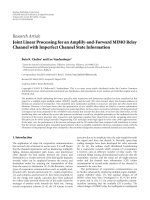
Figure 1: Schematic drawing of the antenna array with (a) and w ithout (b) the displacement of the phase center relative to the orig in of the
coordinate system. Rotating the antenna array (solid) an angle θ gives a relative change (dashed) that depends on the distance to the origin
(δ
x
, δ
y
).
2. DATA MODEL AND PROBLEM FORMULATION
Consider a uniform linear antenna array with M elements
having an interelement spacing of d. A narrowband sig nal,
s(t), is emitted by a point source with direction-of-arrival θ
relative to the broadside of the receiving array. The data col-
lected by the array with true array response
a(θ)is[5, 14]
x
= a(θ)s(t)+w, x ∈ C
M×1

.
(1)
We model
a(θ) as follows:
a(θ)  Ca(θ)e
jk(δ
x
cos θ+δ
y
sin θ)
f (θ), a ∈ C
M×1
,
(2)
where the following conditions hold.
(i)
a(θ) is the true radiation pattern in the far-field includ-
ing mutual coupling, edge effects, and mechanical er-
rors.
a(θ) is modelled as suggested by (2).
(ii) C is the M
× M coupling matrix. This matrix is
complex-valued and unstructured. The main focus of
this paper is to estimate C.
(iii)
{δ
x
, δ
y
} is the array phase center. Figure 1 illustrates

how the displacement of the antenna array is modelled
by δ
x
x + δ
y
y from the origin. The proposed approach
also estimates
{δ
x
, δ
y
}. Note that {δ
x
, δ
y
} is not in-
cluded in the models used in [5, 14].
(iv) f (θ)
≥ 0 is the element factor (antenna radiation
pattern describing the real-valued amplitude of the
electric field pattern) in direction θ without mutual
coupling and describes the amount of radiation from
the individual antenna elements of the array in differ-
ent directions θ. f (θ) is real-valued and includes no
direction-dependent phase shift [7]. The proposed es-
timator also estimates f (θ). Note that f (θ) was not in-
cluded in the models used in [5, 14]. All antenna ele-
ments are implicitly assumed to have equal radiation
patterns when not in an array configuration, that is,
f (θ) is the same for all M elements. When the elements

are placed in an array, the radiation patterns of each
element are not the same due to the mutual coupling.
However , f (θ) is allowed to be nonisotropic, which is
also the case in practice.
(v) a(θ) is a Vandermonde vector whose mth element is
a
m
(θ) = e
jkdsin θ(m−M/2−1/2)
. (3)
(vi) d is the distance between the antenna elements.
(vii) k is the wave number.
(viii) w is i.i.d complex Gaussian noise with zero-mean and
variance σ
2
per element.
Based on calibration data, when a signal, s(t)
= 1, is trans-
mitted from N known direction-of-arrivals
1
{θ
1
, , θ
N
},we
collect one data vector x
n
of measurements for each an-
gle θ
n

. The measurements are arranged in a matrix, X =
[x
1
··· x
N
], as follows:
X
= CAD

δ
x
, δ
y

E

f (θ)

+ W,
A
=

a

θ
1

··· a

θ

N

,
E

f (θ)

=
diag

f

θ
1

, , f

θ
N

,
D

δ
x
, δ
y

=
diag


e
jk(δ
x
cos θ
1
+δ
y
sin θ
1
)
, , e
jk(δ
x
cos θ
N
+δ
y
sin θ
N
)

.
(4)
The matrix W represents measurement noise, which is as-
sumed to be i.i.d zero-mean complex Gaussian with variance
σ
2
per element. In this paper, we propose a method to esti-
mate C when δ

x
, δ
y
,and f (θ)areunknown.
One of the novel aspects of the proposed estimator is the
inclusion of the element factor, f (θ), as a jointly unknown
parameter during the estimation of the coupling matrix, C.
This requires a parametrization that provides a flexible and
mathematically appealing representation of an a priori un-
known element factor. We have chosen to model f (θ)asa
linear combination of sinusoidal basis functions according
to
f (θ)
=
K

k=1
α
k
cos(k − 1)θ, |θ| <
π
2
,(5)
1
Theorientationofthearrayisassumedtobeperfectlyknown,whilethe
exact position of the phase center is typically unknown during the an-
tenna calibration.
Marc Mowl
´
er et al. 3

where K is a known (small) integer, and α are unknown and
real-valued constants. Equation (5)iseffectively equivalent
to a truncated Fourier series where the coefficients are to be
estimated. Even though the chosen parametrization may as-
sume negative values, it is introduced to allow the element
factor, E, to assume arbitrary shapes that can match the true
pattern of the measured antenna array. This can increase the
accuracy in the estimate of C compared to only assuming
an omnidirectional element factor that would correspond to
E
= I.
Other alternative parameterizations of f (θ) exist as well.
A piecewise constant function of θ is one example. The pro-
posed parametrization, on the other hand, is particularly at-
tractive since the basis functions are or thogonal and at the
same time smooth. Additionally, the unknown coefficients,
α
k
, enter the model linearly. Based on (5), the element factor
can be expressed as
E
=
K

k=1
α
k
Q
k
,

α
=

α
1
··· α
K

T
,
Q
k
= diag

cos(k − 1)θ
1
, ,cos(k − 1)θ
N

.
(6)
The coefficients, α, will be jointly estimated together with the
coupling matrix and phase center by the estimator proposed
in this paper.
3. THE PROPOSED ESTIMATOR
We propose to estimate C, α, δ
x
,andδ
y
from X by using a

least-squares criterion
2
on the data model expressed in (4)
according to
min
C,α,δ
x
,δ
y


X − CAD

δ
x
, δ
y

E(α)


2
F
. (7)
Under the assumption of Gaussian noise, (7) is the
maximum-likelihood estimator. The values of C, α, δ
x
, δ
y
that minimize the Frobenius norm in (7) are found using an

iterative approach. The coupling matrix, the matrix C is first
expressed as if the other parameters were known followed by
a minimization over the α parameters while keeping C and
{δ
x
, δ
y
} fixed. A second minimization is made over {δ
x
, δ
y
}
with C and α treated as constants after which the algorithm
loops back to minimize over α again. The steps of the estima-
tor are as follows:
(1) minimize (7) with respect to the coupling matrix, C,
while the phase center,
{δ
x
, δ
y
}, and the element fac-
tor representation, α, are fixed. This is done using the
pseudoinverse approach expressed by [4]

C = X(ADE)
H

ADE(ADE)
H


−1
;(8)
2
The minimum of this cost function is not unique, see Section 4 for a dis-
cussion of this.
(2) minimize (7)withrespecttoα while C, δ
x
,andδ
y
are
fixed. In this step, the value of C found in the previ-
ous step is used as the assumed constant value for the
coupling matrix; the minimization over α is then per-
formed using the following manipulations: first, re-
arrange the measurement mat rix, X, and the expres-
sion (4)invectorizedformas
x
=

vec

Re{X}

vec

Im{X}


,

Y
=

vec

Re

CADQ
1

···
vec

Re

CADQ
K

vec

Im

CADQ
1

} ···
vec

Im


CADQ
K


;
(9)
the least-squares criterion used is then expressed as
min
α


x − Yα


2
F
(10)
with the solution
α =

Y
T
Y

−1
Y
T
x,
(11)
which gives the minimizing α parameters;

(3) minimize (7)withrespecttoδ
x
and δ
y
while keeping
C and α fixed. Using the α parameters found in the
previous step, C, is expressed again according to (8).
Assuming the other parameters to be constant, a two-
dimensional gradient search is conducted to find the
minimizing
{δ
x
, δ
y
} of (7). Steps 1–3 are iterated until
X −

CA

D

E
2
F
is within a certain tolerance level.
To provide the algorithm with an initial estimate, in the first
iteration, we take D
= I and α = [0,1,0, ,0]
T
,whichcor-

responds to the element factor f (θ)
= cosθ that was used in
[13]. The initialization of the algorithm could of course be
done in many different ways and this may affect its perfor-
mance. The choice considered here can be seen as a refine-
ment of the algorithm previously proposed in [13].
Typically, about 5 iterations of the algorithm are required
to reach a local optimum depending on the given tolerance
level. Convergence to the global optimum can not be assured;
however, the algorithm will converge since the cost function
(7) is nonincreasing in each iteration. The topic has been ad-
dressed in previous conference papers [13].
4. CRAM
´
ER-RAO BOUND ANALYSIS
The parameter K, corresponding to the number of terms
used in the t runcated Fourier series representation of the ele-
ment factor, is key to the proposed estimator. This value will
affect the accuracy of the estimator. Increasing the value will
give a better match between the true element factor and the
assumed model. At the same time, it will increase the com-
plexity of the model and complicate the estimation. Another
aspect is the fact that increasing the value K towards infin-
ity may not be the best way of tuning the algor ithm if the
true value is much less. This would force the estimator to use
a model far more complicated than needed, leading to esti-
mation of additional parameters. Even though the parame-
ters would be close to zero, the performance of the estima-
tor is still affected as indicated by the CRB analysis in this
4 EURASIP Journal on Wireless Communications and Networking

section. On the other hand, a smaller number of parameters
may give insufficient flexibility to the algorithm and force it
into a nonoptimal result.
To compensate for the affected performance associated
with a large value of K, the number of measurements N of x
n
can be used as well as a higher signal-to-noise ratio (SNR).
Let us now study the tradeoff between these three parame-
ters by quantifying how the choice of K relates to N and the
SNR (1/σ
2
). The Cram
´
er-Rao bound (CRB) for the estima-
tion problem in (7) is derived and will provide a lower bound
on the variance of the unknown parameters [15–17]. All the
elements of C are considered to be unknown complex-valued
parameters and therefore separated with respect to real and
imaginary parts with C
R
ij
denoting the real part of the element
in the ith row and jth column, and C
I
ij
denoting the corre-
sponding imaginary part. All the 2M
2
+2+K real-valued
unknown parameters of (4) are collected into the vector

ξ
=

C
R
11
··· C
R
1M
··· C
R
MM
··· C
I
ij
δ
x
δ
y
α
1
··· α
K

T
.
(12)
The CRB for the estimate of ξ is expressed by [15]
[CRB]
=


I
Fisher

−1
, (13)
where I
Fisher
is the Fisher information matrix given by

I
Fisher

ij
=
2
σ
2
Re

∂μ
H
∂ξ
i
∂μ
∂ξ
j

,
(14)

where μ is the expected value of x in (9). The problem (7)
is unidentifiable as presented. The scaling ambiguity present
between C and α is solved by enforcing a constraint on the
problem. Here, we choose to constrain
C
2
F
= M as op-
posed to other possibilities such as α
1
= 1orC
R
11
= 1. The
latter favors particular elements of C or α by forcing these
to be nonzero. This is undesirable and consequently ruled
out. This constraint was also implemented as a normaliza-
tion in the estimator presented in the previous section, while
not mentioned there explicitly.
The CRB under parametric constraints is found by fol-
lowing the results derived in [18]. The constraint is expressed
as
g(ξ)
=C
2
F
− M = Tr

C
H

C

−
M = 0.
(15)
Defining

G(ξ)

l
=
∂g(ξ)
∂ξ
l
=
⎧
⎪
⎪
⎨
⎪
⎪
⎩
2Re

c
ij

if ξ
l
= Re


c
ij

,
2Im

c
ij

if ξ
l
= Im

c
ij

,
0 otherwise,
(16)
the constrained CRB is given by [18]
[CRB]
= U(U
T
I
Fisher
U)
−1
U
T

, (17)
where U is implicitly defined via G(ξ)U
= 0. Note that the
CRB is proportional to σ
2
, that is, the estimation accuracy is
inversely proportional to the SNR.
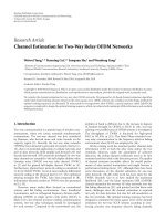
θ
d
h
gp
Figure 2: Schematic overview of the antenna array consisting of
dipoles over an infinite ground plane. The distance from the ground
plane is h
gp
and the spacing between the elements is d. The angle
from the normal to the antenna axis is denoted by θ.
5. RESULTS
5.1. Dipole array example
First, let us consider the case of an 8-element dipole array
over a ground plane, see Figure 2. In the absence of mutual
coupling, each element has the true radiation pattern
E
true
= sin

kh
gp
cos θ


,
(18)
where k is the wave number and h
gp
is the distance to the
ground plane. Using known expressions for mutual coupling
between dipoles [7], it is straightforward to calculate the em-
bedded element patterns. Figures 3(a) and 3(b) show the ra-
diation pattern for a single element and an 8-element array
with mutual coupling for h
gp
= 3λ/8. The interelement spac-
ing is d
= λ/2 and the true {δ
x
, δ
y
} are {0, 0}.
We now compare our proposed method using a trun-
cated Fourier series expansion of the element factor, see (5),
to results obtained by using a cosine-shaped (E
= cos
n
θ)
element pattern assumption as in [13]. In our proposed
method, the algorithm described in Section 3 is used to es-
timate C,
{α
1
, α

2
, α
3
},and{δ
x
, δ
y
}, which corresponds to
choosing K
= 3 in the model for the element factor as ex-
pressed in (5). Similarly, the parameter n in the expression
E
= cos
n
θ is optimized as part of the procedure when us-
ing the method of [13]. In both cases, we make a starting as-
sumption that
{δ
x
, δ
y
}={0, 0}, which is also the tr ue value
for this case.
With no compensation, the uncompensated radiation
pattern is represented in Figure 3(b). With compensation,
where a cosine-shaped element pattern (E
= cos
n
θ)is
assumed, the re sulting radiation pattern is displayed in

Figure 3(c). The unknown values in addition to the mutual
coupling matrix were estimated to
n = 0.5and{

δ
x
,

δ
y
}=
{
0, 0}, and the performance is significantly improved over
the uncompensated case. By allowing the model for the el-
ement factor to follow a truncated Fourier series (K
= 3)
according to our method, the performance of the mutual
coupling matrix estimate is improved even more resulting
in the graph of Figure 3(d). For this case, our method esti-
mated the values for the auxiliary unknown parameters to be
α = [−1.13.1 − 1.1]
T
and {

δ
x
,

δ
y

}={0, 0}. The result also
agrees well with the true (ideal) radiation pattern when the
mutual coupling is neglected as presented in Figure 3(a).
The phase error for the cases of uncompensated and
compensated phase diagrams are presented in Figure 4.The
top graph represents the uncompensated case, while the
Marc Mowl
´
er et al. 5
−20
−15
−10
−5
0
5
Radiation patterns (dB)
−90 −60 −30 0 30 60 90
θ (degrees)
(a) True radiation patterns for a single element; f (θ)
−20
−15
−10
−5
0
5
Radiation patterns (dB)
−90 −60 −30 0 30 60 90
θ (degrees)
(b) Uncompensated radiation patterns with mutual coupling;
x

1
··· x
M
−20
−15
−10
−5
0
5
Radiation patterns (dB)
−90
−60 −30 0 30 60 90
θ (degrees)
(c) Radiation patterns obtained from compensated data using a C
matrix estimated via E
= cos
n
θ as the parametrization of the ele-
ment factor [13]; C
−1
cos
x
1
··· C
−1
cos
x
M
−20
−15

−10
−5
0
5
Radiation patterns (dB)
−90
−60 −30 0 30 60 90
θ (degrees)
(d) Compensated radiation patterns using our method with K = 3;
C
−1
x
1
··· C
−1
x
M
Figure 3: Compensation for mutual coupling for an array of 8 dipoles placed h
gp
= 3λ/8 over a ground plane.
middle and bottom graphs represent compensated cases with
a cosine-shaped and the truncated Fourier series parameter-
izations of the element factors, respectively. This also verifies
that our method with K
= 3 improves the result over con-
straining the element factor to be cosine-shaped (E
= cos
n
θ)
as was proposed in previous work [13].

5.2. CRB for dipole array example
The CRB as a function of K (i.e., the order of the
parametrization of f (θ)) for an 8-element array of dipoles
over ground plane is presented in Figure 5. When generating
this figure, we used the theoretical models of [7] for the cou-
pling between antenna elements with inter-element spacing
d
= λ/2. The true data used are based on a scenario when
K
= 1, D = I,andE = I.TheSNRwas0dB(σ
2
= 1). The
four curves show
(i) CRB
C
= Tr{{U
C
(U
T
C
I
C
U
C
)
−1
U
T
C
}

C
}, the CRB of C
when both D and E are known;
(ii) CRB
CD
= Tr{{U
CD
(U
T
CD
I
CD
U
CD
)
−1
U
T
CD
}
C
}, the CRB
of C when D is unknown and E is known;
(iii) CRB
CE
= Tr {{U
CE
(U
T
CE

I
CE
U
CE
)
−1
U
T
CE
}
C
}, the CRB of
C when D is known and E is unknown;
(iv) CRB
CDE
= Tr {{U
CDE
(U
T
CDE
I
CDE
U
CDE
)
−1
U
T
CDE
}

C
}, the
CRB of C when D and E are unknown.
The results in Figure 5 quantify the increase in achievable es-
timation performance for the elements of C when increasing
the number of nuisance parameters in the model. In partic-
ular, we see that the estimation problem becomes more dif-
ficult when more α parameters are introduced in the model.
For example, it is more difficult to estimate the coupling ma-
trix C when the phase center δ
x
, δ
y
, is unknown. However,
6 EURASIP Journal on Wireless Communications and Networking
X
−50 −25 0 25 50
θ (deg)
−10
0
10
(a)
C
−1
cos
n
X
−50 −25 0 25 50
θ (deg)
−10

0
10
(b)
C
−1
X
−50 −25 0 25 50
θ (deg)
−10
0
10
(c)
Figure 4: Uncompensated (a) and compensated (b, c) phase dia-
grams with E
= cos
n
θ and E =

α
k
Q
k
,respectively.Thetrue
element factor is E
true
= sin(2π(3/8)cosθ), which corresponds to
h
gp
= 3λ/8.
for K ≥ 3, the difficulty of identifying α dominates over

the problem of estimating the phase center. Since the CRB is
proportional to σ
2
, the increase in emitter power (i.e., SNR)
required to maintain a given performance when the model
is increased with more unknowns can be seen in the fig-
ure.
In Figure 6, the CRB as a function of K and N is stud-
ied. From this figure, we can directly read out how much
higher emitter power (or equivalently, lower σ
2
)isrequired
to be able to maintain the same estimation perfor mance for
C when K or N vary. For example, if fixing N
= 100, say,
then going from K
= 1toK = 2 requires 1 dB additional
SNR. Going from K
= 2toK = 3 requires an increase of
the SNR level by 1.5 dB. However, going from K
= 3to4
requires 10 dB extra SNR. Thus, K
= 3 appears to be a rea-
sonable choice. In practice, it is difficult to handle more than
K
= 3 for the element factor in this case.
In Figure 6, we observe that in the limit when the number
of angles reaches N
= 15, the problem becomes unidentifi-
able. This is so because for N

≤ 15 the number of unknown
parameters in the model exceeds the number of recorded
samples. From Figure 6 many other interesting observations
can be made. For instance, increasing N from 100 to 200, for
afixedK, is approximately equivalent to increasing the SNR
with 3 dB. This holds in general: for N
 1, doubling the
SNR gives the same effect as doubling N.
−26
−24
−22
−20
−18
−16
−14
−12
1234
K
CRB (dB)
CRB
CDE
CRB
CE
CRB
CD
CRB
C
Figure 5: The CRB for the elements of C under different assump-
tions on whether D, E are known or not, and for different K. SNR
is 0 dB.

−25
−20
−15
−10
15 50 100 150 200
N
CRB (dB)
K = 1
K
= 2
K
= 3
K
= 4
Figure 6: The CRB for the elements of C as a function of K and N
when SNR is 0 dB.
5.3. Measured results on a dual polarized array
Next, let us study the performance of the proposed estima-
tor on an ac tual antenna array. Data from an 8-column an-
tenna array (see Figure 7) were collected at 1900 MHz dur-
ing calibration measurements with 180 measurement points
distributed evenly over the interval θ
∈{−90
◦
··· 90
◦
}.
Uncompensated radiation patterns with mutual coupling are
presented in Figure 8 for measured data of the array. The es-
timator presented in this paper was used to estimate the cou-

pling matrix. The estimated coupling matrix was then used
Marc Mowl
´
er et al. 7
Figure 7: Eight-column dual polarized array developed by Pow-
erwave Technologies Inc. Results are presented for this array in
Section 5.3. Note that each vertical column of radiators forms an
element with pattern
a
m
(θ) in the horizontal plane.
to precompensate the data, after which radiation patterns can
be obtained.
To modify our estimator (Section 3) to the dual polarized
case, we follow [14]. Considering a dual polarized array with
±45
◦
polarization and neglecting noise, (4)becomes

x
−45
◦
co
x
−45
◦
xp
x
+45
◦

xp
x
+45
◦
co

=

C
11
ADE
1
C
12
ADE
2
C
21
ADE
2
C
22
ADE
1

, (19)
where x
−45
◦
co

means measuring the incoming −45
◦
polarized
signal with the antenna elements of the same polarization,
while x
−45
◦
xp
means the data measured at the −45
◦
element
when the incoming signal is +45
◦
. To estimate the total cou-
pling matrix,
C
tot
=

C
11
C
12
C
21
C
22

, (20)
the four blocks of (19) are treated independently according

to
x
−45
◦
co
= C
11
ADE
1
, x
−45
◦
xp
= C
12
ADE
2
,
x
+45
◦
xp
= C
21
ADE
2
, x
+45
◦
co

= C
22
ADE
1
.
(21)
The D matrices of these four independent equations are
equal. The E
1
matrix represents the copolarization blocks of
(19), namely, x
−45
◦
co
and x
+45
◦
co
, simultaneously and is mod-
elled according to (5) with a set of α para meters estimated by
our method. For the cross-polarization, we assume isotropic
element patterns, E
2
= I. Once the equations in (21)are
solved, the total coupling matrix can be expressed using (20)
and the radiation pattern of the measured data may be com-
pensated by inverting the coupling matrix according to
⎡
⎣
x

−45
◦
compensated
x
+45
◦
compensated
⎤
⎦
=
C
−1
tot
⎡
⎣
x
−45
◦
measured
x
+45
◦
measured
⎤
⎦
. (22)
Figure 8(a) shows the individual radiation patterns of
each antenna element as measured during calibration (x).
Figure 8(b) shows the radiation patterns after compensation
by the coupling matrix (C

−1
iso
X) when isotropic conditions are
assumed by the estimator. This means assuming E
= I,which
is equivalent to setting K
= 1 in our algorithm. The radiation
patterns after compensation by the coupling matrix when
using the proposed estimator with K
= 3arepresentedin
Figure 8(c).
The results using an isotropic assumption on the element
factor, Figure 8(b), shows an improvement over the uncom-
pensated data of Figure 8(a). The graphs showing the copo-
larization (solid) are smoother and more equal to each other,
which is what is expected from an array with equal elements
when no coupling is present. The cross-polarization (dashed)
is suppressed significantly compared to the uncompensated
case. The estimated phase center is
{

δ
x
,

δ
y
}=[0.20].
Further improvement is achieved using our proposed
method, Figure 8(c). Using K

= 3, our method estimates the
coefficients in the element factor representation (5)as
α =
[0.8 − 0.40.6] and the phase center as {

δ
x
,

δ
y
}=[0.30].
The resulting compensated radiation pattern of Figure 8(c)
is even closer to the ideal array response when no coupling
is assumed. The copolarization graphs are almost overlap-
ping in the
±60
◦
interval showing the radiation patterns of
8 equal elements with cosine-like element factors. The cross-
polarization is also improved slightly over the isotropic case.
Phase diagrams representing the average phase error of
the coupling matrix before and after compensation with the
coupling matrix are presented in Figure 8(d).Thephaseer-
ror after compensation with K
= 3(Figure 8(d),bottom),
modelling the phase shift and the element factor, is less than
without the compensation (Figure 8(d), top). Assuming an
isotropic element factor (Figure 8(d),middle)givesabetter
result than without compensation but not as good as the re-

sult of our method. This indicates that the validity of the es-
timated coupling matrix based on phase considerations in-
creases with the proposed estimator. Furthermore, the results
of our method with K
= 3 show a notable improvement over
the results presented in [14].
6. K-VALUE TRADEOFF BASED ON
MONTE CARLO SIMULATIONS
We have seen in Section 5.2 that there is a tradeoff between
K, N, and the SNR in terms of the CRB. In reality, the er-
ror in the estimation is a combination of both model- and
noise-induced errors. Let us therefore study the overall per-
formance of our proposed estimator using the root-mean-
square error of the mutual coupling matrix:
RMS
=
1
M
2
C −

C
F
=
1
M
2





ij


C
ij
−

C
ij


2
, (23)
where M
2
is the number of elements in C. As an example,
we use an 8-element linear array with spacing d
= λ/2and
a true element factor given by α
true
= [0010 ]
T
.Simu-
lations were conducted with our method for K
= 1 5
based on 1000 realizations and an SNR
= 30 dB. The result
is shown in Figure 9. The CRB for the given SNR level is also
8 EURASIP Journal on Wireless Communications and Networking

−25
−20
−15
−10
−5
0
Radiation patterns (dB)
−50 0 50
θ (degrees)
(a) Measured uncompensated radiation patterns for the array of
Figure 7;
{x
−45
◦
measured
, x
+45
◦
measured
}
T
−25
−20
−15
−10
−5
0
Radiation patterns (dB)
−50 0 50
θ (degrees)

(b) Radiation patterns obtained from compensated data using a C
matrix estimated via our algorithm setting K
= 1 (i.e., forcing E ∝
I); C
−1
iso
{x
−45
◦
measured
, x
+45
◦
measured
}
T
−25
−20
−15
−10
−5
0
Radiation patterns (dB)
−50 0 50
θ (degrees)
(c) Compensated radiation patterns using our method with K = 3;
C
−1
{x
−45

◦
measured
, x
+45
◦
measured
}
T
−50 −25 0 25 50
θ (degrees)
−10
0
10
−10
0
10
−10
0
10
c)
b)
a)
(Deg)
(d) Phase errors for the cases in (a), (b), and (c)
Figure 8: Radiation patterns obtained from compensated data with the coupling matrix C estimated in different ways. The measurements
are from the 8-element dual polarized array in Figure 7 with co- (solid) and cross- (dashed) polarization collected during calibration.
presented in the same graph and represents the impact of the
noise. This is seen as an increase of the CRB in the region
K>3.
Because of the insufficient parametrization of E, the RMS

is higher for smaller values of K than the true K. The RMS
decreases toward the point where K
= 3,whichisthetrue
value of K. For higher values of K, there is no longer a model
error and the noise is the sole contributor to the RMS. This
is evident as an increase in RMS when K>3. The same
estimation was also made with E
= cos
n
θ [13]. A straight
line represents this case in Figure 9 showing the difference in
RMS, which is higher compared to using our method with
K
= 3. This shows that the optimum tradeoff for our pro-
posed method, in this case, is K
= 3. This g ives the best
performance when comparing different values of K and the
E
= cos
n
θ assumption.
7. CONCLUSIONS
We have introduced a new method for the estimation of the
mutual coupling matrix of an antenna arr ay. The main nov-
elty over existing methods was that the array phase center
and the element factors were introduced as unknowns in the
data model, and treated as nuisance parameters in the esti-
mation of the coupling as well, by being jointly estimated to-
gether with the coupling matrix.
In a simulated test case, our method outperformed

the previously proposed estimator [13 ] for the case of an
Marc Mowl
´
er et al. 9
0
0.01
0.02
0.03
0.04
0.05
0.06
12345
K
RMS
RMS
cos
0.5
RMS
K=3
CRB
Figure 9: CRB and RMS based on Monte Carlo simulations when
SNR is 30 dB. The true element factor is E
true
= cos2θ, which means
α
true
= [0010 0]orK
true
= 3.
8-element dipole array. The radiation pattern and phase er-

ror were significantly improved leading to increased accuracy
in any following postprocessing.
Based on a CRB analysis, the SNR penalty associated with
introducing a model for the element factor with two degrees
of freedom (K
= 3) was 2.5 dB relative to having zero de-
grees of freedom. This means that an additional 2.5 dB more
power (or a doubling of the number of accumulated sam-
ples) must be used to retain the estimation accuracy of the
coupling mat rix compared to the case when the algorithm
assumed omnidirectional elements. To add another degree
of freedom (set K
= 4) costs another 10 dB.
Using measured calibration data from a dual polarized
array, we found that the proposed method and the associated
estimator could significantly improve the quality of the esti-
mated coupling matrix, and the result of subsequent com-
pensation processing.
Finally, the tradeoff between the complexity of the pro-
posed data model and the accuracy of the estimator was stud-
ied via Monte Carlo simulations. For the case of an 8-element
linear array, the optimum was found to be at K
= 3which
coincides with the t rue value in that case.
ACKNOWLEDGMENTS
This material was presented in part at ICASSP 2007 [19]. Erik
G. Larsson is a Royal Swedish Academy of Sciences Research
Fellow supported by a grant from the Knut and Alice Wallen-
berg Foundation.
REFERENCES

[1] D.TseandP.Viswanath,Fundamentals of Wireless Communi-
cation, Cambridge University Press, Cambridge, UK, 2005.
[2] A. Swindlehurst and T. Kailath, “A performance analysis of
subspace-based methods in the presence of model errors—
part I: the MUSIC algorithm,” IEEE Transactions on Signal Pro-
cessing, vol. 40, no. 7, pp. 1758–1774, 1992.
[3] M. Jansson, A. Swindlehurst, and B. Ottersten, “Weighted sub-
space fitting for general array error models,” IEEE Transactions
on Signal Processing, vol. 46, no. 9, pp. 2484–2498, 1998.
[4]B.FriedlanderandA.J.Weiss,“Effects of model errors
on waveform estimation using the MUSIC algorithm,” IEEE
Transactions on Signal Processing, vol. 42, no. 1, pp. 147–155,
1994.
[5] H. Steyskal and J. S. Herd, “Mutual coupling compensation
in small array antennas,” IEEE Transactions on Antennas and
Propagation, vol. 38, no. 12, pp. 1971–1975, 1990.
[6] J. Yang and A. L. Swindlehurst, “The effects of array calibration
errors on DF-based signal copy performance,” IEEE Transac-
tions on Signal Processing, vol. 43, no. 11, pp. 2724–2732, 1995.
[7] C. A. Balanis, Antenna Theory: Analysis and Design,JohnWiley
& Sons, New York, NY, USA, 1997.
[8] T. Svantesson, “The effects of mutual coupling using a linear
array of thin dipoles of finite length,” in Proceedings of the 9th
IEEE SP Workshop on Statistical Signal and Array Processing
(SSAP ’98), pp. 232–235, Portland, Ore, USA, September 1998.
[9] K. R. Dandekar, H. Ling, and G. Xu, “Effect of mutual cou-
pling on direction finding in smart antenna applications,”
Electronics Le tters, vol. 36, no. 22, pp. 1889–1891, 2000.
[10] B. Friedlander and A. Weiss, “Direction finding in the pres-
ence of mutual coupling,” IEEE Transactions on Antennas and

Propagation, vol. 39, no. 3, pp. 273–284, 1991.
[11] T. Su, K. Dandekar, and H. Ling, “Simulation of mutual cou-
pling effect in circular arrays for direction-finding applica-
tions,” Microwave and Optical Technology Letters, vol. 26, no. 5,
pp. 331–336, 2000.
[12] B. Lindmark, S. Lundgren, J. Sanford, and C. Beckman, “Dual-
polarized array for signal-processing applications in wireless
communications,” IEEE Transactions on Antennas and Propa-
gation, vol. 46, no. 6, pp. 758–763, 1998.
[13] M. Mowl
´
er and B. Lindmark, “Estimation of coupling, ele-
ment factor, and phase center of antenna arrays,” in Proceed-
ings of IEEE Antennas and Propagation Society International
Symposium, vol. 4B, pp. 6–9, Washington, DC, USA, July 2005.
[14] B. Lindmark, “Comparison of mutual coupling compensation
to dummy columns in adaptive antenna systems,” IEEE Trans-
actions on Antennas and Propagation, vol. 53, no. 4, pp. 1332–
1336, 2005.
[15] S. M. Kay, Fundamentals of Statistical Signal Processing: Esti-
mation Theory, Prentice-Hall, Upper Saddle River, NJ, USA,
1993.
[16] H. L. Van Trees, Detection, Est imation, and Modulation Theory,
Wiley-Interscience, New York, NY, USA, 2007.
[17] J. Gorman and A. Hero, “Lower bounds for parametric estima-
tion with constraints,” IEEE Transactions on Information The-
ory, vol. 36, no. 6, pp. 1285–1301, 1990.
[18] P. Stoica and B. C. Ng, “On the Crame
´
er-Rao bound under

parametric constraints,” IEEE Signal Processing Letters, vol. 5,
no. 7, pp. 177–179, 1998.
[19] M. Mowl
´
er, E. G. Larsson, B. Lindmark, and B. Ottersten,
“Methods and bounds for antenna array coupling matrix es-
timation,” in Proceedings of IEEE International Conference on
Acoustics, Speech, and Signal Processing (ICASSP ’07), vol. 2,
pp. 881–884, Honolulu, Hawaii, USA, April 2007.