Báo cáo hóa học: " Research Article Hop-Distance Estimation in Wireless Sensor Networks with Applications to Resources Allocation Liang Zhao and Qilian Liang" pot

Hindawi Publishing Corporation
EURASIP Journal on Wireless Communications and Networking
Volume 2007, Article ID 84256, 8 pages
doi:10.1155/2007/84256
Research Article
Hop-Distance Estimation in Wireless Sensor
Networks with Applications to Resources Allocation
Liang Zhao and Qilian Liang
Department of Electrical Engineering, University of Texas at Arlington, Arlington, TX 76010, USA
Received 22 May 2006; Revised 7 December 2006; Accepted 26 April 2007
Recommended by Huaiyu Dai
We address a fundamental problem in wireless sensor networks, how many hops does it take a packet to be relayed for a given
distance? For a deterministic topology, this hop-distance estimation reduces to a simple geometry problem. However, a statisti-
cal study is needed for randomly deployed WSNs. We propose a maximum-likelihood decision based on the conditional pdf of
f (r
| H
i
). Due to the computational complexity of f (r | H
i
), we also propose an attenuated Gaussian approximation for the
conditional pdf. We show that the approximation visibly simplifies the decision process and the error analysis. The latency and
energy consumption estimation are also included as application examples. Simulations show that our approximation model can
predict the latency and energy consumption with less than half RMSE, compared to the linear models.
Copyright © 2007 L. Zhao and Q. Liang. This is an open access article distributed under the Creative Commons Attribution
License, which permits unrestricted u se, distribution, and reproduction in any medium, provided the original work is properly
cited.
1. INTRODUCTION
The recent advances in MEMS, embedded systems, and wire-
less communications enable the realization and deployment
of wireless sensor networks (WSN), which consist of a large
number of densely deployed and self-organized sensor nodes

[1]. The potential applications of WSN, such as environment
monitor, often emphasize the importance of location infor-
mation. Fortunately, with the advance of localization tech-
nologies, such location information can be accurately esti-
mated [2–5]. Accordingly, geographic routing [6–8]waspro-
posed to route packets not to a specific node, but to a given
location. An interesting question arises as “how many hops
does it take to reach a given location?” The prediction of the
number of hops, that is, hop-distance estimation, is impor-
tant not only in itself, but also in helping, estimate the latency
and energy consumption, which are both important to the
viability of WSN.
The question could become very simple if the sensor
nodes are manually placed. However, if sensor nodes are de-
ployed in a random fashion, the answer is beyond the reach
of simple geometry. The stochastic nature of the random de-
ployment calls for a statistical study.
The relation between the Euclidean distance and network
distance (in terms of the number of hops), also referred to
as hop-distance relation, catches a lot of research interest re-
cently. In [9], Huang et al. defined the Γ-compactness of a
geometric graph G(V,E) to be the minimum ratio of the Eu-
clidean distance to the network distance,
γ
= min
i, j∈V
d(i, j)
h(i, j)
,(1)
where d(i, j)andh(i, j) are the Euclidean distance and net-

work distance between nodes i and j,respectively.Thecon-
stant value γ is a good lower bound, but might not be enough
to describe the nonlinear relation between Euclidean distance
and network distance. In fact, their relation is often treated as
linear for convenience, for example, [r/R] + 1 is widely used
to estimate the needed number of hops to reach distance r
given transmission range R. Against this simple intuition, the
relation between Euclidean distance and network distance is
far more complex. Fortunately, a lot of probabilistic stud-
ies have been applied to this question. In [10], Hou and Li
studied the 2D Poisson distribution to find an optimal trans-
mission range. They found that the hop-distance distribu-
tion is determined not only by node density and transmission
range, but also by the routing strategy. They showed results
for three routing strategies, most forward with fixed radius,
nearest with forward progress, and most forward with vari-
able radius. Cheng and Robertazzi in [11] studied the one-
dimensional Poisson point and found the pdf of r given the
number of hops. They also pointed out that the 2D Poisson
2 EURASIP Journal on Wireless Communications and Networking
point distribution is analogous to the 1D case, replacing the
length of the segment by the area of the range. Vural and
Ekici reexamined the study under the sensor networks cir-
cumstances in [12], and gave the mean and variance of mul-
tihop distance for 1D Poisson point distribution. They also
proposed to approximate the multihop distance using Gaus-
sian distribution. Zorzi and Rao derive the mean number of
hops of the minimal hop-count route through simulations
and analytic bounds in [8]. Chandler [13] derives an expres-
sion for t-hop outage probability for 2D Poisson node distri-

bution. However, Mukherjee and Avidor [14] argue that one
of Chandler’s assumptions is relaxed, and thus his expression
is in fact a lower bound on the desired probability. Using
the same assumption, the y also derive the pdf of the mini-
mal number of hops for a given distance in a fading envi-
ronment. Although these analytic results are available in the
literature, their monstrous computational complexity limits
their applications. Therefore, we try to approximate the hop-
distance relation and simplify the decision process and error
analysis in this paper. Considering the application of resource
allocation, only large-scale path loss is considered, and thus
the fading is ignored.
The rest of this paper is organized as follows. The num-
ber of hops prediction problem is addressed and solved in
Section 2. Since this problem has no closed-form solution,
we propose an attenuated Gaussian approximation and show
how to simplify the error analysis in Section 2.1.Application
examples are shown in Section 3. Section 4 concludes this pa-
per.
2. ESTIMATION OF NETWORK DISTANCE BASED ON
EUCLIDEAN DISTANCE
Suppose the sensor nodes are placed on a plane at random,
and N(A),thenumberofnodesinagivenareaA,follows
two-dimensional Poisson distribution with average density
λ. The problem of interest is to find the number of hops
needed to reach a distance r away. We can make a maximum-
likelihood (ML) decision,

H = arg max f


r | H
n

, n = 1, 2, 3, ,(2)
where the event H
n
can be described as “the minimum num-
ber of hops is n from the source to the specific node at Eu-
clidean distance r.” In the following discussion, we are trying
to approximate f (r
| H
n
) for 2D Poisson distribution. Note
that r<Rimplies H
1
, that is, the specific node is w ithin one
hop from the source. We are more interested in multiple-hop
distance relation, especially when n is moderately large.
2.1. Attenuated Gaussian approximation
Since f (r
| H
i
) is awkward to evaluate even using numeri-
cal methods, we use histograms collected from Monte Carlo
simulations as substitute to the joint pdf. All the simulation
data are collected from a scenario where N sensor nodes were
uniformly distributed in a circular region of radius of R
Bound
meters. For convenience, polar coordinates were used. The
source node was placed at (0, 0). The transmission range was

Table 1: Statistics of f (r | H
i
).
Number of hops Mean STD Skewness Kurtosis
1 19.991 7.0651 −0.57471 −0.58389
2 45.132 7.8365
−0.16958 −1.0763
3 72.01 8.2129
−0.10761 −1.0332
4 99.45 8.391
−0.07938 −0.97857
5 127.14 8.5323
−0.06445 −0.93104
6 154.96 8.6147
−0.05341 −0.9004
7 182.68 8.573
−0.07738 −0.91687
0
0.01
0.02
0.03
0.04
0.05
0.06
0.07
Histogram
0 20 40 60 80 100 120 140 160 180 200
r(m)
Figure 1: Histograms of hop-distance joint distribution (N = 1000,
R

Bound
= 200, R = 30).
set as R meters. For each setting of (N, R
Bound
, R), we ran 300
simulations, in each of which all nodes are redeployed at ran-
dom. We ran simulations for extensive settings of node den-
sity λ and transmission range R. Due to space constraints,
only the histograms for (N
= 1000, R
Bound
= 200, R =
30) are plotted in Figure 1, which approximately shows that
f (r
| H
i
) approaches the normal when H
i
increases. Ta ble 1
lists the first-, second-, third-, and fourth-order statistics of
f (H, r).
Skewness is a third-order statistic used to measure of
symmetry, or more precisely, the lack of symmetry. Skewness
is zero for a symmetric distribution and positive skewness in-
dicates right skewness while negatives indicates left skewness.
Definition 1 (see [15]). For a given sample set X,
m
3
=
Σ(X − X)

3
n
,
m
2
=
Σ(X − X)
2
n
,
(3)
where
X is the sample mean of X,andn is the size of X. Then
a sample estimate of skewness coefficient is given by
g
1
=
m
3
m
3/2
2
. (4)
L. Zhao and Q. Liang 3
0
0.005
0.01
0.015
0.02
0.025

0.03
0.035
0.04
0.045
Histogram
30 40 50 60 70 80
r(m)
(a)
0
0.005
0.01
0.015
0.02
0.025
0.03
0.035
0.04
Histogram
40 50 60 70 80 90 100 110
r(m)
(b)
0
0.005
0.01
0.015
0.02
0.025
0.03
0.035
Histogram

60 70 80 90 100 110 120 130 140
r(m)
(c)
0
0.005
0.01
0.015
0.02
0.025
0.03
0.035
Histogram
80 90 100 110 120 130 140 150 160 170
r(m)
(d)
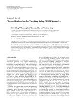
Figure 2: The histogram versus postulated distribution for end-to-end distances for given number of hops: (a) three hop; (b) four hop; (c)
five hop; (d) six hop.
Kurtosis is a fourth-order statistic indicating whether the
data are peaked or fl at relative to a normal distribution.
Definition 2 (see [15]). A sample estimate of kurtosis for a
sample set X is given by
g
2
=
m
4
m
2
2
− 3, (5)

where m
4
= Σ(X − X)
4
/n is the fourth-order moment of X
about its mean.
Skewness and kurtosis are useful in determining whether
a sample set is normal. Note that the skewness and kurtosis
of a normal distribution are both zero; significant skewness
and kurtosis clearly indicate that data are not normal. Tab le 1
clearly shows that the skewness and kurtosis satisfy the Gaus-
sianity condition within tolerance of error. Furthermore, The
postulated distribution and histogram are drawn together in
Figures 2(a), 2(b), 2(c),and2(d), which clearly shows a close
match for each case. Also, note that f (r
| H
n
)attenuatesex-
ponentially with n increase, we need to int roduce an attenu-
ation factor to model this behavior.
Thus, the objective function can be approximated by
f

r | H
n

=
α
n
N


m
n
, σ
n

=
α
n
2πσ
e
−(r−m
n
)
2
/2σ
2
n
,(6)
where α is the equivalent attenuation base, m
n
and σ
n
are
the mean and standard deviation (STD), respectively. Since
f (r
| H
n
) attenuates with n increasing, α must be less than 1.
The specific values of these parameters can be estimated from

simulations or computed numerically from the exact pdfs.
Our extensive simulations show that even for only moder-
ately large H
i
, f (r | H
i
) has the following properties.
(1) σ
n
≈ σ
n−1
, which means that the neighboring joint
pdfs have similar spread.
4 EURASIP Journal on Wireless Communications and Networking
H
n−1
H
n
H
n+1
d
n−1
d
n
r
Figure 3: Gaussian approximation.
(2) m
n
− m
n−1

≈ m
n+1
− m
n
, which means that the joint
pdfs are evenly spaced.
(3) 3 < (m
n
− m
n−1
)/σ
n
< 5, which means the overlap be-
tween the neighboring joint pdfs is small but not neg-
ligible. (As a rule of thumbs, Q(3) is considered rela-
tively small and Q(5) is regarded negligible.)
(4) (m
n
− m
n−2
)/σ
n
 5, which means the overlap be-
tween the nonneighboring joint pdfs is negligible.
(5) α<1. For large density λ, α
→ 1. Along with prop-
erty (1), this tell us that the neighboring joint pdfs have
nearly identical shape.
As shown in the following discussion, these proper ties largely
simplify the decision rule and the error analysis. Another in-

teresting observation, besides these properties, is that the fol-
lowing equations do not stand tr ue,
m
n
= nm
1
,
m
n
= nR,
m
n
= (n − 1)R + R/2.
(7)
Although these equations sound plausible, they all give vis-
ible errors. The aforementioned estimator [r/R]+1forH
i
,
though widely used, is not good in the new light shed by this
study.
2.2. Decision boundaries
Following (2), and observing the f (r
| H
i
)inFigure 3, the
decision is needed only between neighboring H
i
, that is,
f


r | H
n

n
≷
n+1
f

r | H
n+1

. (8)
This is because, for a specific value of r, there are only two
values of H
i
with dominating f (r | H
i
), compared to which
f (r
| H
i
) for other values of H
i
is neglig ible. Substituting
(6) into (8), we obtain the decision boundary d
n
between the
regions H
n
and H

n+1
,
d
n
=
B +
√
B
2
+ AC
A
,
A
= σ
2
n+1
− σ
2
n
,
B
= m
n
σ
2
n+1
− m
n+1
σ
2

n
,
C
= m
2
n
σ
2
n+1
− m
2
n+1
σ
2
n
+2σ
2
n
σ
2
n+1
ln α.
(9)
Using property (1),
d
n
=
m
2
n+1

− m
2
n
− 2σ
2
n
ln α
2

m
n+1
− m
n

. (10)
For large density λ, property (5) is applicable, (9) simplifies
to
d
n
=
σ
2
n
m
n+1
+ σ
2
n+1
m
n

σ
2
n
+ σ
2
n+1
. (11)
Applying property (1) to (11),
d
n
=
m
n
+ m
n+1
2
. (12)
No matter which approximate solution we choose for d
n
, the
decision rule is given by
r
n+1
≷
n
d
n
. (13)
In other words,
we decide

n if d
n−1
<r≤ d
n
. (14)
2.3. Error performance analysis
For our decision rule, a decision error occurs only when the
required number of hops is n, but our decision
n/=n.Thus,
the probability of error for a specific r is
p(
 | r) =

n/=

n
f

H
n
| r

, (15)
where f (H
| r) is related to f (r | H
i
) by the Bayesian rule.
The total probability of error is obtained by integrating (15)
over all possible r,
p(

) =

p( | r) f
r
(r)dr. (16)
According to property (4), only f (r
| H = n − 1) and f (r |
H = n + 1) could have outstanding value over the decision
region [d
n−1
, d
n
],
p(
) ≈
∞

n=2

d
n
d
n−1
f

r | H
n−1

p


H
n−1

+ f

r | H
n+1

p

H
n+1

dr
=
∞

n=2
α
n−1
p

H
n−1


Q

d
n−1

−m
n−1
σ
n−1

−
Q

d
n
− m
n−1
σ
n−1

+α
n+1
p

H
n+1


Q

m
n+1
−d
n
σ

n+1

−
Q

m
n+1
−d
n−1
σ
n+1

.
(17)
L. Zhao and Q. Liang 5
Note that
d
n
− m
n−1
σ
n−1
−
d
n−1
− m
n−1
σ
n−1
=

d
n
− d
n−1
σ
n−1
 1, (18)
therefore, Q((d
n
− m
n−1
)/σ
n−1
)isnegligiblecomparedto
Q((d
n−1
− m
n−1
)/σ
n−1
). Similarly, Q((m
n+1
− d
n
)/σ
n+1
)is
neglig ible. Equation (17) is approximated by
p(
) ≈ α

3
p

H
3

Q

m
3
− d
2
σ
3

+
∞

n=3

α
n−1
p

H
n−1

Q

d

n−1
− m
n−1
σ
n−1

+ α
n+1
p

H
n+1

Q

m
n+1
− d
n
σ
n+1

=
α
2
p

H
2


Q

d
2
− m
2
σ
2

+
∞

n=3
α
n
p

H
n


Q

m
n
− d
n−1
σ
n


+ Q

d
n
− m
n
σ
n

.
(19)
Substituting an appropriate solution of d
n
into (19)would
give us the probability of error within required accuracy. For
example, if we choose (12),
p(
) ≈ α
2
p

H
2

Q

m
3
− m
2

2σ
2

+
∞

n=3
α
n
p

H
n


Q

m
n
− m
n−1
2σ
n

+ Q

m
n+1
− m
n

2σ
n

.
(20)
Thanks to the Gaussian approximation, the error probabil-
ity is given in forms of Q functions, which is tremendously
simpler than the derivation from the original pdfs. This er-
ror process is general and applicable to other estimators. For
example, even when we have to use a linear estimator due
to limit of computation capacity, we can still use the above
process to obtain the corresponding error probability.
3. APPLICATION EXAMPLES
We provide two application examples, latency and energy es-
timation, in this section. To emphasize the role of the num-
ber of hops in the estimation, we use general time and energy
models. On how to derive the parameters such as T
rx
, T
tx
for
a specific routing scheme, readers are referred to [16, 17].
3.1. Latency estimation
We use a simple time model, in which the latency increases
linearly with the number of hops [18]. Suppose it takes T
rx
,
T
tx
for a sensor node to process 1 bit of incoming and out-

going messages, respectively, and T
pr
is the required time to
transmit 1 bit of message through a band-limited channel.
Therefore, the latency introduced for each hop is
T
hop
= T
tx
+ T
pr
+ T
rx
. (21)
mT
rx
mT
tx
···
T
pr
Figure 4: Time model.
Table 2: Energy consumption parameters
Name Value
r
0
86.2 m
E
elec
50 nJ/bit

E
DA
5 nJ/bit

fs
10 pJ/bit/m
2

mp
0.0013 pJ/bit/m
4
As shown in Figure 4, given the end-to-end distance r,wecan
find the required number of hops
n according to (13), thus,
a good estimator of the total latency of an l-bit message is
l
nT
hop
. (22)
3.2. Energy consumption estimation
Thefollowingmodelisadoptedfrom[19] where perfect
power control is assumed. To transmit l bits over distance
r, the sender’s radio expends
E
tx
(l, r) =
⎧
⎨
⎩
lE

elec
+ l
fs
r
2
, r<d
0
,
lE
elec
+ l
mp
r
4
, r ≥ d
0
,
(23)
and the receiver’s radio expends
E
rx
(l, r) = lE
elec
. (24)
E
elec
is the unit energy consumed by the electronics to pro-
cess one bit of message,

fs

and 
mp
are the amplifier factor
for free-space and multipath models, respectively, and d
0
is
the reference distance to determine which model to use. In
fact, the first branch of (23) assumes a free-space propaga-
tion and the second branch uses a path-loss exponent of 4.
The values of these communication energy parameters are
set as in Tab le 2.
Let s
n
denote the single-hop distance from the (n −1)th-
hop to the nth-hop. Obviously, s
n
≤ R.Inourexperimental
setting, R
= 30m<d
0
so that the free-space model is al-
ways used. This agrees well with most applications, in which
multihop short-range transmission is preferred to avoid the
exponential increase in energy consumption for long-range
transmission. Naturally, the end-to-end energy consumption
for sending l bit over distance r is given by
E
total
(l, r) =
n


1

E
tx

l, r
1

+ E
rx
(l)

, (25)
6 EURASIP Journal on Wireless Communications and Networking
2
3
4
5
6
7
8
9
Average (latency)
40 60 80 100 120 140 160 180 200
r
Actual
Statistical
Linear 1
Linear 2

(a)
2
3
4
5
6
7
8
9
×10
−7
Average (energy consumption)
40 60 80 100 120 140 160 180 200
r
Actual
Statistical
Linear 1
Linear 2
(b)
Figure 5: Estimation average: (a) latency; (b) energy consumption.
where n is the estimated number of hops for given r and r
1
is the single-hop distance because the message is relayed hop
by hop .
On the average,
E
total
(l, r) = nl

E

elec
+ 
fs
E

r
2
1

+ E
elec

= 
nl

2E
elec
+ 
fs

m
2
1
+ σ
2
1

.
(26)
3.3. Simulation

We used the same scenario described in Section 2.1 and var-
ied the node density λ and transmission range R.Ineachsim-
ulation, the number of hops is estimated for each node using
(11)and(13), and then the latency and energy consumption
are estimated using (22)and(26), respectively. As compar-
ison to our proposed statistic-based estimator, we choose a
widely used linear estimator,
linear estimator 1
n =

r
R

+1,
linear estimator 2
n =

r
R

+2,
(27)
where r is the given distance, R, the transmission range, and
[r/R] is the maximum integer less than r/R. We plot the av-
erage of latency and energy consumption in Figures 5(a) and
5(b) and the RMSE in Figures 6(a) and 6(b),respectively.The
latency is plotted in units of T
hop
while the energy consump-
tion in units of joules. The ripple shape of RMSE is due to the

fact that decision errors occur more often in the overlapping
zones of neighboring f (r
| H
i
). Figure 5 shows that the linear
estimator 1 performs well at the shorter range but suffers vis-
ibly at larger range, while the linear estimator does the oppo-
site. The linear estimators, no matter what value their param-
eters take, may significantly underestimate or overestimate
the latency and energy consumption as already pointed out
in Section 2.1, while our statistic-based model keeps close to
the actual latency and energy consumption at all ranges ex-
cept for the border. This is also verified by Figure 6,which
also shows that our model can reduce RMSE to at least half
for both latency and energy consumption. These results show
that linear models cannot identify network behavior accu-
rately, as also confirmed by our extensive simulations for dif-
ferent settings of node density and transmission range, which
is not shown here due to space constraints.
4. CONCLUSION
To address the fundamental problem “how many hops does
it take for a packet to be relayed for a given distance,” we
make both probabilistic and statistical studies. We proposed
a Bayesian decision based on the conditional pdf of f (r
| H
i
).
Since f (r
| H
i

) is computationally complex, we also pro-
posed an attenuated Gaussian approximation for the condi-
tional pdf, which visibly simplifies the decision process and
the error analysis. This error analysis based on Gaussian ap-
proximation is also applicable to other estimators, includ-
ing the linear ones. We also show that several linear mod-
els, though intuitively sound and widely used, may give sig-
nificant bias er ror. Given as application examples, our ap-
proximation is also applied in the latency and energy con-
sumption estimation in dense WSN. Simulations show that
our approximation model can predict the latency and energy
L. Zhao and Q. Liang 7
0
0.2
0.4
0.6
0.8
1
1.2
1.4
1.6
1.8
2
RMSE (latency)
40 60 80 100 120 140 160 180 200
r
Statistical
Linear 1
Linear 2
(a)

0
0.2
0.4
0.6
0.8
1
1.2
1.4
1.6
1.8
2
×10
−7
RMSE (energy consumption)
40 60 80 100 120 140 160 180 200
r
Statistical
Linear 1
Linear 2
(b)
Figure 6: Estimation RMSE: (a) latency; (b) energy consumption.
consumption with less than half RMSE, compared to the
aforementioned linear models.
ACKNOWLEDGMENT
This work was supported by the US Office of Naval Research
(ONR) Young Investigator Award under Grant N00014-03-
1-0466.
REFERENCES
[1] I. F. Akyildiz, W. Su, Y. Sankarasubramaniam, and E. Cayirci,
“A survey on sensor networks,” IEEE Communications Maga-

zine, vol. 40, no. 8, pp. 102–114, 2002.
[2] H. Lim and J. C. Hou, “Localization for anisotropic sensor net-
works,” in Proceedings of the 24th Annual Joint Conference of
the IEEE Computer and Communications Societies (INFOCOM
’05), vol. 1, pp. 138–149, Miami, Fla, USA, March 2005.
[3] A. Caruso, S. Chessa, S. De, and A. Urpi, “GPS free coordinate
assignment and routing in wireless sensor networks,” in Pro-
ceedings of the 24th Annual Joint Conference of the IEEE Com-
puter and Communications Societies (INFOCOM ’05), vol. 1,
pp. 150–160, Miami, Fla, USA, March 2005.
[4] L. Fang, W. Du, and P. Ning, “A beacon-less location discovery
schemeforwirelesssensornetworks,”inProceedings of the 24th
Annual Joint Conference of the IEEE Computer and Communi-
cations Societies (INFOCOM ’05), vol. 1, pp. 161–171, Miami,
Fla, USA, March 2005.
[5] N. B. Priyantha, H. Balakrishnan, E. D. Demaine, and S.
Teller, “Mobile-assisted localization in wireless sensor net-
works,” in Proceedings of the 24th Annual Joint Conference of
the IEEE Computer and Communications Societies (INFOCOM
’05), vol. 1, pp. 172–183, Miami, Fla, USA, March 2005.
[6] R. Jain, A. Puri, and R. Sengupta, “Geographical routing using
partial information for wireless ad hoc networks,” IEEE Per-
sonal Communications, vol. 8, no. 1, pp. 48–57, 2001.
[7] Y. Xu, J. Heidemann, and D. Estrin, “Geogr aphy-informed en-
ergy conservation for ad hoc routing,” in Proceedings of the
7th Annual International Conference on Mobile Computing and
Networking (MOBICOM ’01), pp. 70–84, ACM Press, Rome,
Italy, July 2001.
[8] M. Zorzi and R. R. Rao, “Geographic random forwarding
(GeRaF) for ad hoc and sensor networks: multihop perfor-

mance,” IEEE Transactions on Mobile Computing, vol. 2, no. 4,
pp. 337–348, 2003.
[9] Q. Huang, C. Lu, and G C. Roman, “Spatiotemporal mul-
ticast in sensor networks,” in Proceedings of the 1st Interna-
tional Conference on Embedded Networked Sensor Systems (Sen-
Sys ’03), pp. 205–217, ACM Press, Los Angeles, Calif, USA,
November 2003.
[10] T C. Hou and V. O. K. Li, “Transmission range control in mul-
tihop packet radio networks,” IEEE Transactions on Communi-
cations, vol. 34, no. 1, pp. 38–44, 1986.
[11] Y C. Cheng and T. G. Robertazzi, “Critical connectivit y phe-
nomena in multihop radio models,” IEEE Transactions on
Communications, vol. 37, no. 7, pp. 770–777, 1989.
[12] S. Vu ral and E. Ekici, “Analysis of hop-distance relationship
in spatially random sensor networks,” in Proceedings of the 6th
ACM Internat ional Symposium on Mobile Ad Hoc Networking
and Computing (MOBIHOC ’05), pp. 320–331, ACM Press,
Urbana-Champaign, Ill, USA, May 2005.
[13] S. A. G. Chandler, “Calculation of number of relay hops re-
quired in randomly located radio network,” Electronics Letters,
vol. 25, no. 24, pp. 1669–1671, 1989.
[14] S. Mukherjee and D. Avidor, “On the probability distribution
of the minimal number of hops between any pair of nodes
in a bounded wireless ad-hoc network subject to fading,” in
8 EURASIP Journal on Wireless Communications and Networking
Proceedings of the 2nd International Workshop on Wireless Ad-
Hoc Networks (IWWAN ’05), London, UK, May 2005.
[15] G. Snedecor and W. Cochran, Statistical Methods,IowaState
University Press, Ames, Iowa, USA, 1989.
[16] M. Zorzi and R. R. Rao, “Geographic random forwarding

(GeRaF) for ad hoc and sensor networks: energy and latency
performance,” IEEE Transactions on Mobile Computing, vol. 2,
no. 4, pp. 349–365, 2003.
[17] H. M. Ammari and S. K. Das, “Trade-off between energy sav-
ings and source-to-sink delay in data dissemination for wire-
less sensor networks,” in Proceedings of the 8th ACM Sympo-
sium on Modeling, Analysis and Simulation of Wireless and Mo-
bile Syste ms (MSWiM ’05), pp. 126–133, ACM Press, Montreal,
Quebec, Canada, October 2006.
[18] W. Ye, J. Heidemann, and D. Estrin, “Medium access control
with coordinated adaptive sleeping for wireless sensor net-
works,” IEEE/ACM Transactions on Networking, vol. 12, no. 3,
pp. 493–506, 2004.
[19] W. B. Heinzelman, A. P. Chandrakasan, and H. Balakrishnan,
“An application-specific protocol architecture for wireless mi-
crosensor networks,” IEEE Transactions on Wireless Communi-
cations, vol. 1, no. 4, pp. 660–670, 2002.