Báo cáo hóa học: " Research Article Iterative Desensitisation of Image Restoration Filters under Wrong PSF and Noise Estimates" pot

Hindawi Publishing Corporation
EURASIP Journal on Advances in Signal Processing
Volume 2007, Article ID 72658, 18 pages
doi:10.1155/2007/72658
Research Article
Iterative Desensitisation of Image R estoration Filters under
Wrong PSF and Noise Estimates
Miguel A. S antiago,
1
Guillermo Cisneros,
1
and Emiliano Bernu
´
es
2
1
Depart amento de Se
˜
nales, Sistemas y Radiocomunicaciones, Escuela T
´
ecnica Superior de Ingenieros de Telecomunicaci
´
on,
Universidad Polit
´
ecnica de Madrid, 28040 Madr id, Spain
2
Departamento de Ingenier
´
ıa Electr
´

onica y Comunicaciones, Centro Polit
´
ecnico Superior, Universidad de Zaragoza,
50018 Zaragoza, Spain
Received 19 July 2005; Revised 30 November 2006; Accepted 3 January 2007
Recommended by Bernard C. Levy
The restoration achieved on the basis of a Wiener scheme is an optimum since the restoration filter is the outcome of a minimisa-
tion process. Moreover, the Wiener restoration approach requires the estimation of some parameters related to the original image
and the noise, as well as knowledge about the PSF function. However, in a real restoration problem, we may not possess accurate
values of these parameters, making results relatively far from the desired optimum. Indeed, a desensitisation process is required to
decrease this dependency on the parameter errors of the restoration filter. In this paper, we present an iterative method to reduce
the sensitivity of a general restoration scheme (but s pecified to the Wiener filter) wi th regards to wrong estimates of t he said pa-
rameters. Within the Fourier transform domain, a sensitivity analysis is tackled in depth with the purpose of defining a number of
iterations for each frequency element, which leads to the aimed desensitisation regardless of the errors on estimates. Experimental
computations using meaningful values of parameters are addressed. The proposed technique effectively achieves better results than
those obtained when using the same w rong estimates in the Wiener approach, as well as verified on an SAR restoration.
Copyright © 2007 Miguel A. Santiago et al. This is an open access article distributed under the Creative Commons Attribution
License, which permits unrestricted use, distribution, and reproduction in any medium, provided the original work is properly
cited.
1. INTRODUCTION AND BACKGROUND
Let h be any generic two-dimensional degradation filter mask
(PSF, usually invariant low-pass filter). Let x be an original
image to be degraded. A generic linear shift-invariant degra-
dation process of x using h can be written in a general way
as
y
= h ∗∗x + n,(1)
where y is the degraded image (blurred and noisy im-
age), and n is a two-dimensional matrix representing the
added noise in the degradation. A restoration procedure will

achieve a replica
x of the original image x. The inversion of
the degradation process cannot be derived directly; funda-
mentals on image processing [1–3] provide further details on
this ill-posed problem. Therefore, a number of approaches
have been investigated in the image restoration arena [4].
The classical stochastic regularisation method for image
restoration minimises a global restoration error ε by means
of the function
ε
= min

E


y − y
2

,(2)
where E
{·} represents the expectation operator.
Assuming circular convolution, as well as a stationary
model for the blur h, the original image x, and the indepen-
dent noise n, the said minimisation provides an optimum
linear solution written as a scalar operation for each 2D fre-
quency component (ω
i
, ω
j
) in the Fourier transform domain

(using DFT) as

X

ω
i
, ω
j

=
G

ω
i
, ω
j

Y

ω
i
, ω
j

=
H
∗

ω
i

, ω
j



H

ω
i
, ω
j



2
+ C

ω
i
, ω
j

Y

ω
i
, ω
j

(3)

which is the Wiener restoration approach stood for the well-
known Wiener filter G where

X = DFT(x), Y = DFT(y),
2 EURASIP Journal on Advances in Signal Processing
H = DFT(h), and C represents somehow an SNR parameter
given by
C

ω
i
, ω
j

=
S
nn

ω
i
, ω
j

S
xx

ω
i
, ω
j


,(4)
where S
xx
and S
nn
are the respective spec tral densities of the
original image x and the noise matrix n.
On the basis of (3), the stochastic regularisation ap-
proach fully depends on a priori knowledge about h, x,and
n. Regarding h, lots of work have been addressed to achieve
estimates of the PSF, for example, [5–14]. On the other hand,
common assumptions consider Gaussian noise for S
nn
and
presume that the spec tral density S
xx
of the unavailable or ig-
inal image x is not very different from the spectral density
S
yy
of the degraded image y, therefore S
xx
∼
=
S
yy
[4]. How-
ever, it is important to point out other techniques for prior
image modelling such as the use of Gauss-Markov random

fields [15–18] or the wavelets models [19–21].
The more correct those estimates are, the closer the
restoration result of (3) is to the optimum solution of (2).
Nevertheless, the sensitivity of (3)towrongestimatesis
very high; for example, relatively small deviations from the
real (unknown) value of C make (3) yield results very far
from the desired optimum. State-of-art provides some al-
gorithms of robust filters [22–24], particularly addressed
to obtain good results in spite of the presence of outliers
within the noise (when expected to be Gaussian). Nonethe-
less, our objective is not to obtain an independent filter,
but to improve the results of an original restoration (rela-
tive procedure) when having wrong estimates of the depen-
dant parameters. That is to say, we aim to provide the orig-
inal restoration with robustness in a paramet rical sense by
means of a desensitisation process. Additionally, a large liter-
ature can be found regarding researches on iterative restora-
tion (e.g., [25–32]) as an alternative to solve this prob-
lem.
In order to simplify notation, the reference to the element
(ω
i
, ω
j
) of the matrices in the frequency domain will be re-
moved from all formulae throughout the remainder of this
paper. Besides, it must be taken into account that all mathe-
matical expressions involving matrices in the Fourier trans-
form domain will be scalar computations for each frequency
component (ω

i
, ω
j
).
Moreover, since we use estimates of the parameters in the
restoration side, let us remark them by including a suffix e all
along the analysis to differ from real values, that is, H
e
and C
e
for the Wiener approach.
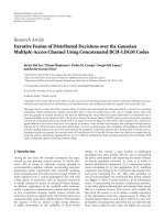
In short, Section 2 proposes an iterative model for de-
sensitisation with respect to the before-mentioned estimates.
Afterwards, Section 3 provides an analysis on the degree of
desensitisation achieved, as well as a proposal for the number
of iterations. Finally, Section 4 offerssomerestorationresults
to present the successful benefits reached by our innovative
restoration scheme.
Y
0
= Y
H
e
G

Y
1
, ,

Y

K
G

X

1
, ,

X

K
=

X

k −→ k +1
G

Figure 1: Proposed restoration scheme.
2. RESTORATION MODEL
In the light of the above, we can write the restored image
(Fourier transform) in a general way as

X = GY = G(HX + N) = GHX + GN,(5)
where N
= DFT(n). Going a step further, our research aims
to build an innovative restoration filter G

based on G whose
sensitivity with respect to the estimates related to the restora-

tion model (such as H
e
and C
e
in the Wiener approach) is
smaller than that of G. This filter G

will provide another
replica
x

of the original image, whose Fourier transform

X

= DFT(x

)canbewrittenas

X

= G

Y = G

(HX + N) = G

HX + G

N. (6)

In order to achieve this purpose, G

is defined by applying
an iterative process of degradations and restorations, using
H
e
and G, respectively. This process is graphically explained
in Figure 1.
The input at any iteration k (k
= 1, 2, , K)isanimage
y
k−1
(Y
k−1
= DFT(y
k−1
)) where Y
0
= Y = HX + N (i.e., to
say, the degraded image y). The corresponding output is an
approach
x

k
to x

(

X


k
= DFT(x

k
)). After the last iteration K,
we will have

X

of (6)as

X

=

X

K
. A criterion will be adopted
to define this total number of iterations K.
Actually, this proposed restoration method is applied
within the Fourier transform domain on the degraded spec-
trum Y and, as stated later, the number of iterations K is a
function of each frequency element, as denoted by the inclu-
sion of the symbol (ω
i
, ω
j
) in the restoration scheme.
Mathematically, the iterative process of Figure 1 is ex-

plained for every frequency pair as follows:

Y
1
= GH
e
Y
0
= GH
e
Y

X

1
= G

Y
1
= G

GH
e

HX
= GH
e
(HX + N)+G

GH

e

N

Y
2
= GH
e

Y
1

X

2
= G

Y
2
= G

GH
e

2
HX
=

GH
e


2
(HX + N)+G

GH
e

2
N
Miguel A. Santiago et al. 3

Y
3
= GH
e

Y
2

X

3
= G

Y
3
= G

GH
e


3
HX
=

GH
e

3
(HX + N)+G

GH
e

3
N
.
.
.
.
.
.

Y
k
= GH
e

Y
k−1


X

k
= G

Y
k
= G

GH
e

k
HX
=

GH
e

k
(HX + N)+G

GH
e

k
N
.
.

.
.
.
.

Y
K
= GH
e

Y
K−1

X

K
= GY
K
= G

GH
e

K
HX
=

GH
e


K
(HX + N)+G

GH
e

K
N =

X

.
(7)
By comparing (6) with any row (right side) of (7), we can
write our proposed desensitisation filter G

at any iteration k
and for each frequency element (ω
i
, ω
j
)as
G

= G

GH
e

k

. (8)
Having a look to (8), we can verify the dependency of the
new filter G

on three basic parameters such as the original
restoration filter G (e.g., the Wiener approach), the regular-
isation product GH
e
(different from the original regularisa-
tion GH) as explained in the restoration regularisation the-
ory [33–35], and the number of iterations k of the model
shown in Figure 1.
Therefore, our goal now aims to demonstrate the desen-
sitisation behaviour of our proposed restoration filter G

,
showing which conditions lead to successful results, pur-
posely, the total number of iterations K applied to each pair
(ω
i
, ω
j
). A first approach to this idea was initially coped with
in [ 36 ] where some preliminary results meant opening steps
to the current fully study throughout this paper.
3. SENSITIVITY OF THE FILTERS
3.1. Condition establishment
Let us now compute and compare the sensitivities of G and
G


with respect to the estimates and assumptions required in
the restoration process. Let S
G
be the sensitivity regarding the
filter G which can be defined as
S
G
=
∂G
∂P
1
dP
1
+
∂G
∂P
2
dP
2
+ ···+
∂G
∂P
n
dP
n
,(9)
where P
1
, P
2

, , P
n
are the parameters to be estimated in the
restoration model. For instance, H
e
and C
e
stand for the re-
quired estimates in the Wiener restoration method within
the Fourier domain which involve the before-mentioned pa-
rameters in the introductory section, explicitly, the PSF func-
tion h (H
e
) and the original image x, and the noise n (C
e
).
Indeed, this Wiener approach will be coped with in the re-
mainder of this paper in order to present both mathematical
analysis and computed results. Hence, we can rewrite (9)as
S
G
=
∂G
∂H
e
dH
e
+
∂G
∂C

e
dC
e
. (10)
Analogously, the sensitivity concerning the proposed fil-
ter G

can be expressed as follows:
S

G
=
∂G

∂H
e
dH
e
+
∂G

∂C
e
dC
e
. (11)
Multiplying and dividing (11)by∂G

, both sensitivities
(10)and(11) can be related to each other as

S

G
=
∂G

∂G

∂G
∂H
e
dH
e
+
∂G
∂C
e
dC
e

=
∂G

∂G
S
G
. (12)
After differentiating the filter G

with respect to G tak-

ing the expression (8) into account, we come up with a mile-
stone concept within our research into restoration sensitivity,
namely, the relative sensitivity function of G

regarding G for
a given pair (ω
i
, ω
j
)denotedbyZ(k) whose definition can be
described as
Z(k)
=
S

G
S
G
=
∂G

∂G
=
∂
∂G

G

GH
e


k

=
(k +1)

GH
e

k
.
(13)
Consequently, we find the condition for the proposed fil-
ter G

to be less sensitive than G with regards to wrong as-
sumptions of H
e
and wrong estimates of C
e
as
S

G
<S
G
⇐⇒ Z(k) < 1. (14)
As a corollary, this condition (14) can be extended to not
only a global sensitivity study but also a focusing of the anal-
ysis on a particular estimation of the restoration model re-

gardless of which one is considered. Thus, taking (9) into
consideration, let us define the sensitivity of the filter G with
respect to the parameter P as S
P
G
,
S
P
G
=
∂G
∂P
. (15)
Comparing both sensitivities S
P
G
and S
P
G
yields
S
P
G

S
P
G
=
∂G


/∂P
∂G/∂P
=
∂G

∂G
= Z(k). (16)
Hence, this leads to the conclusion stated by the corollary
S

G
<S
G
⇐⇒ Z(k) < 1 ⇐⇒ S
P
G

<S
P
G
(17)
applied to whatsoever parameter of the restoration approach,
particularly, H
e
and C
e
within our Wiener method.
3.2. Condition analysis
As a first step of our analysis, let us consider the regularisa-
tion term GH

e
involved in the expression (13). In view of (3),
this product can be rewritten as
GH
e
=
H
∗
e
H
e
H
∗
e
H
e
+ C
e
=


H
e


2


H
e



2
+ C
e
. (18)
4 EURASIP Journal on Advances in Signal Processing
Z(k)
3
2.5
2
1.5
1
0.5
0
0 5 10 15 20 25
k
GH
e
= 0.85
GH
e
= 0.75
GH
e
= 0.65
GH
e
= 0.35
Figure 2: Relative sensitivity function Z(k).

By definition, in the presence of noise, that is to say, real
restoration conditions,
S
nn
|
e
> 0, S
xx
|
e
≥ 0 =⇒ C
e
=
S
nn
|
e
S
xx
|
e
> 0 ∀

ω
i
, ω
j

.
(19)

Taking for granted that
|H
e
|
2
≥ 0 and combining (19)
into ( 18), the product GH
e
can be ranged as fol lows:
0
≤GH
e
<1 =⇒ 0≤

GH
e

k
≤GH
e
<1 ∀

ω
i
, ω
j

, ∀k ≥1.
(20)
As a result of (20), we can conclude that the relative sen-

sitivity function Z(k)
= (k +1)(GH
e
)
k
of (13) is not either
monotonically increasing or decreasing with the number of
iterations k, but it may show a relative maximum extreme,
depending on the value of the term GH
e
for a particular pair
(ω
i
, ω
j
). This is illustrated in Figure 2 for several regularisa-
tion values.
From the last plot, we find the expected maximum ex-
tremes of Z(k) as peaks located on specific numbers of itera-
tions k depending on which regularisation value GH
e
is con-
sidered. Clearly, the lower the product GH
e
is, the less itera-
tions k are required to reach the consequent less intensified
maximum of Z(k). Furthermore, high enough regularisation
conditions (i.e., to say, low values of GH
e
)makeZ(k)fully

decreasing monotonic.
Nonetheless, the main conclusion to be drawn from
Figure 2 is related to the sensitivity condition (14), once im-
posing an identity Z(k)-level over the graphic, which shows
the iteration from which the appointed desensitisation is
achieved. In fact, looking at the plot, we can say that regard-
less of the value of the product GH
e
, G

is less sensitive than
G if the number of iterations k is high enough. Under this
hypothesis, we may increase the value of k as much as wished
in order to prevent poor restoration results under wrong esti-
mates of the implied parameters (H
e
and C
e
). Unfortunately,
this statement is not true since there are other restoration fac-
tors to be considered. Precisely, next section deals with this
issue.
3.3. Condition limits
The goal of this section is to analyse the proposed filter G

from a view based on the restoration error in order to ver-
ify how the desensitisation influences the final results. Thus,
let E
t
be the Fourier Transform of the restoration error with

regards to our proposed model whose expression is
E

t
=

X

− X. (21)
Besides, the digital image theory [1–3] divides the
restoration error into two meaningful components as fol-
lows:
E

t
= E

r
+ E

n
, (22)
where E

r
and E

n
are the well-known image-dependent and
noise-dependent components in the Fourier domain, respec-

tively.
By taking (6) into account and comparing both expres-
sions (21)and(22), it leads to
(G

HX + G

N) − X = E

r
+ E

n
. (23)
Consequently, we come up with the definitions of the
restoration error components as
E

r
= (G

H − I)X, E
n
= G

N, (24)
where I represents the identity matrix for every pair (ω
i
, ω
j

).
Analogously, we can rewrite the same expressions regard-
ing the original restoration filter G (Wiener approach) as be-
low:
E
r
= (GH − I)X, E
n
= GN. (25)
However, we are actually interested in contrasting the
restoration errors from both models in order to demonstrate
the influence of the desensitisation on the restored image.
Hence, let δ
r
and δ
n
be the relative image-dep endent and
noise-dependent errors, respectively, as
δ
r
=
E

r
E
r
, δ
n
=
E


n
E
n
. (26)
Substituting (24), (25) into (26), in addition to applying
the definition of our filter G

(8), we have
δ
r
(k) =

G

GH
e

k
H − I

X
(GH − I)X
=
1 − (GH)

GH
e

k

1 − GH
,
δ
n
(k) =
E

n
E
n
=
G

GH
e

k
N
GN
=

GH
e

k
(27)
Miguel A. Santiago et al. 5
δ
r
(k)

3.5
3
2.5
2
1.5
1
0 5 10 15 20 25
k
GH
e
= 0.85
GH
e
= 0.75
GH
e
= 0.65
GH
e
= 0.35
Figure 3: Relative image-dependent error δ
r
(k).
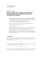
whose plots with respect to the number of iterations k are il-
lustrated in Figures 3 and 4 using the same regularisation val-
ues GH
e
as in Figure 2 and holding fixed the original product
GH to 0.7.
Looking at those figures, we find out the mentioned con-

straint in the last section which prevented increasing un-
boundedly the number of iterations in order to intensify the
desensitisation level as shown in Figure 2. The more we raise
the value of k, the higher the relative image-dependent er-
ror δ
r
and, on the contrar y, the lower the relative noise-
dependent error δ
n
becomes.
Consequently, we are forced to strike a trade-off between
both component errors whether successful desensitisation
results are pretended for a specific v alue of iterations, besides
taking the condition (14) into account.
As a matter of interest, it can be easily demonstrated by
applying the range (20) to the expressions (27), apart from
assuming that the original regularisation GH also fulfills that
range, then,
δ
r
(k) ≥ 1 ∀

ω
i
, ω
j

, ∀k ≥ 1, (28)
0
≤ δ

n
(k) < 1 ∀

ω
i
, ω
j

, ∀k ≥ 1 (29)
which states that the noise-dependent error is always lower
for our proposed restoration model than that of the orig-
inal schema (Wiener approach). Conversely, the image-
dependent error becomes higher giving an evidence of a
much better improvement on very noisy degraded images
than those corrupted by other kind of degradations.
Going a step further, it is important to point out that
the condition (28) is not always satisfied if the said hypothe-
sis regarding GH is not kept. Indeed, when wrong estimates
about the PSF are considered, this product can be over the
unity or even negative making the relative image-dependent
error δ
r
decrease with the number of iterations k. Although it
seems to be another successful result, however, it is not likely
δ
n
(k)
1
0.9
0.8

0.7
0.6
0.5
0.4
0.3
0.2
0.1
0
0 5 10 15 20 25
k
GH
e
= 0.85
GH
e
= 0.75
GH
e
= 0.65
GH
e
= 0.35
Figure 4: Relative noise-dependent error δ
n
(k).
to have this situation too expanded all along the spec trum
when reasonable estimates of H
e
are taken, but if so, the ben-
efits obtained by reducing the image-dependent error are not

enough to improve the extreme impairments caused by the
high deviation from the real value of H.
3.4. Recommended number of iterations
Following the basis on our research, we cope with the task of
working out an appropriate number of iterations K applied
to the proposed model. Let us remind that we are using scalar
computations of matrices in the Fourier domain and, conse-
quently, the obtained number of iterations will be a function
of every pair (ω
i
, ω
j
).
As a result of previous sections, we can see that the in-
crease of the number of iterations k may provide a less sen-
sitive restoration filter G

as desired. Nevertheless, both the
image-dependent and noise-dependent restorations errors
do not al low raising it unboundedly. Thus, we will try to find
arequiredtrade-off.
From the beginning, our goal is to reduce the value of
the relative sensitivity function Z(k) as stated in condition
(14). Since this function does not provide any minimum as
illustrated in Figure 2, let us optimise another Z(k)property
which fulfills our desensitisation purpose. With this in mind,
let us look for a maximum of e fficiency for the incremental
complexity introduced in the restoration process by increas-
ing the number of iterations from k to k + 1. In other words,
let us seek a value of k fromwhichwedonotgetmuchmore

improvements on desensitisation but, on the contrary, the
complexity is notably incremented.
The next step consists of giving a m athematical sense to
this conceptual criterion with regards to Z(k). Knowing that
we can simulate the variation of a function by means of its
derivative, the reduction of sensitivity can be accomplished
through the first derivative of Z(k), namely, Z

(k). In view
6 EURASIP Journal on Advances in Signal Processing
R(k)
0.4
0.2
0
−0.2
−0.4
−0.6
−0.8
−1
0 5 10 15 20 25
k
GH
e
= 0.85
GH
e
= 0.75
GH
e
= 0.65

GH
e
= 0.35
Figure 5: Function R(k) defined as the second derivative of Z(k).
of the fact that the desensitisation change is expected to be
maximised, the second derivative of Z(k) is herein the aimed
function denoted by R(k),
R(k)
= Z

(k) =
∂
2
Z(k)
∂k
2
. (30)
After some calculations (see Appendix A), we obtain the
definition of R(k),
R(k)
=

GH
e

k
ln

GH
e


2+(k +1)ln

GH
e

(31)
whose representation, as illustrated in Figure 5,givesusafull
evidence of the successful approach due to the presence of
maximum extremes.
Therefore, our proposed desensitisation criterion can be
summarized as the value of k which fulfills
max

R(k)

, Z(k) < 1 ∀k ≥ 1. (32)
In Appendix B, it is further demonstrated that the solved
number of iterations K can be expressed as follows:
K
= round

−

1+
3
ln

GH
e



(33)
subject to a constraint on the regularisation term GH
e
,
0.14 <GH
e
< 0.84. (34)
With the purpose of making sure about the successful
criterion, let us present numeric results by means of Table 1
which comes together all the mainly showed concepts such
as GH
e
, K, Z(k), δ
r
(k), and δ
n
(k) (relative errors values are
in dB), leaving the original regularisation GH unalterable to
the value 0.7. Looking at this table, we can see that the im-
provements achieved for δ
n
(k) are greater than the impair-
ments obtained from δ
r
(k), always satisfying the desensiti-
sation condition Z(k) < 1. For that reason, it is expected
to have good restoration results with a rough estimation of
noise in a very wide range, much better than the other kind

of wrong estimates.
4. SIMULATION RESULTS
With the intention of proving the successful benefits achieved
by our innovative restoration model, let us simulate some il-
lustrative examples. Purposely, the image selected for testing
is the well-known Cameraman 256
× 256 sized making eas-
ier to compare the obtained results with those from other
researches in the restoration area.
As stated in Section 1, the original image is disturbed by
a degradation filter and an additive noise. In order to show
a variety of meaningful examples, let us make use of sev-
eral common filters within the application of astronomical
imaging such as the motion blur, the atmospheric turbu-
lence degradation (Gaussian), and the uniform blur. More-
over, both the most typical Gaussian white noise and other
more complicated artefacts such as “salt and pepper” or mul-
tiplicative noises ( speckle) are added to the blurred image.
Thereby, the next subsec tions aim to specify the proposed
restoration method by collecting all these possible options in
such a way that the main goals of our paper can be clearly evi-
denced, that is to say, the improvements accomplished by our
iterative scheme G

on an original restoration filter G when
wrong estimates of the parameters are considered.
Regarding the restoration filter G, as indicated through-
out the paper, the minimum mean-squared method (Wiener
filter) is used and, consequently, H
e

and C
e
are the param-
eters to be estimated. Let us remind that they represent the
frequency estimates of the three generic restoration parame-
ters: the original image and the noise (C
e
) and the degrada-
tion filter (H
e
).
In view of the fact that those parameters must be al-
tered to show the efficacy of the desensitised filter G

,let
us arrange some guidelines to modify each one. Firstly, we
take into consideration the said assumption pointed out in
Section 1 about the original image whose spectral density
S
xx
is roughly approximated by that of the degraded image
S
yy
. Concerning the noise, we assume a Gaussian estimation
whose variance stands for the parameter to be altered. Con-
sequently, the value of C
e
in (4) changes from the real one. Fi-
nally, we consider a motion blur for the degradation estima-
tion H

e
modifying the inclination parameter and the number
of moved pixels. Furthermore, we deal with not only the se-
lection of the same category of input processes, that is to say,
gaussian noise and motion blur as real values, but also with
providing other classes such as commented at the beginning
of this section.
By means of a relative error, we manage to measure
the deviations from the real value of those parameters.
Thus, let ε
P
be the relative error of a gener ic parameter P
defined as follows:
ε
P
=
P
real
− P
estimated
P
real
· 100, (35)
where P
real
and P
estimated
stand for the respective real and es-
timated values of the parameter P.
Miguel A. Santiago et al. 7

Table 1: Numeric results for the functions GH
e
, K, Z(k = K), δ
r
(k = K), and δ
n
(k = K) applied to the desensitisation.
GH 0.20 0.25 0.30 0.35 0.40 0.45 0.50 0.55 0.60 0.65 0.70 0.75 0.80
K 11122334567912
Z(k
= K) 0.40 0.50 0.60 0.37 0.48 0.36 0.50 0.46 0.47 0.53 0.66 0.75 0.89
δ
r
(k = K) 9.15 8.79 8.41 9.68 9.43 9.89 9.66 9.88 9.97 9.99 9.94 9.99 10.03
δ
n
(k = K) −13.98 −12.04 −10.46 −18.24 −15.92 −20.81 −18.06 −20.77 −22.18 −22.45 −21.69 −22.49 −23.26
Let us remark that this relative error is not directly ad-
dressed to the complex and two-dimensional parameters H
e
and C
e
, but applied on other dependent variables such as
the blurring inclination θ or the noise variance σ
2
as pre-
viously mentioned. Provided that these parameters are real
variables, the relative error ε
P
is also extended along the range

−∞ <ε
P
< +∞, even though we only consider the significant
values ranged between
−100 and 100%.
In order to properly show the steps up, the results are al-
ways presented with regards to the Wiener filter when us-
ing optimum estimates; the same when wrong estimates are
taking into account and, finally, by applying our restoration
model under the same mistaken estimates.
Let us remind that the proposed desensitisation mech-
anism yields a different number of iterations for every pair
(ω
i
, ω
j
) due to its dependence on the product GH
e
, which is,
likewise, variable with each frequency component, namely,
K(ω
i
, ω
j
) = K[GH
e
(ω
i
, ω
j

)]. By using the expression of (33),
we obtain a value of K for those pairs whose related regular-
isation term GH
e
is within the range given by (34). Thus, a
criterion will be adopted for choosing a number of iterations
for the rest of frequencies. Owing to the increasing trend of K
with respect to GH
e
(see Table 1), all pairs whose correspond-
ing regularisation value exceeds 0.84 are associated to a con-
stant number of iterations, equal to the maximum value of
K reached by those within the range. Respectively, the min-
imum value of K computed within the range is applied to
those under 0.14, explicitly, no iterations are brought into
play.
Eventually, a way to numerically contrast the restoration
results is obtained by a n image quality parameter named as
the improvements on the signal-to-noise ratio, that is, ISNR,
ISNR
= 10 log


M−1
i=0

N−1
j=1

x( i, j) − y(i, j)


2

M−1
i=0

N−1
j=1

x( i, j) − x(i, j)

2

, (36)
where x(i, j), y(i, j), and x(i, j) represent the M × N sized
images x, y,and
x, respectively. The more similar the restored
image
x is to the original image x, the higher the parameter
ISNR becomes.
Example 1. In a fi rst simulation, we investigate the case
where wrong estimates of the parameter C
e
are considered
and the value of H
e
is not altered with regards to H.
We start applying a motion blur to the original image de-
scribed by a length of 15 pixels and an angle of 45 degrees in
a counter-clockwise direction. Later on, a Gaussian noise is

added following a blurred signal-to-noise ratio BSNR ranged
between 0 and 30 dB.
In the restoration process, we keep the parameter H
e
tak-
ing the same values of the original motion blur. On the other
hand, apart from the fixed error result of the original im-
age estimation S
xx
|
e
∼
=
S
yy
, the parameter C
e
is distorted by
changes in the variance of an estimated Gaussian noise. Ex-
pressly, we evaluate the variations of this parameter using the
relative error of the standard deviation σ associated to the
noise, namely, ε
σ
whose expression can be written using (35)
as
ε
σ
=
σ
real

− σ
estimated
σ
real
· 100. (37)
After solving this equation regarding σ
estimated
,
σ
estimated
= σ
real

1 −
ε
σ
100

, (38)
and replacing the standard deviation σ with the squared as-
sociated variance σ
2
, we can express the estimated variance
as follows:
σ
2
estimated
=



σ
2
real

1 −
ε
σ
100

2
. (39)
On the way to achieve a significant range of results, we
alter the estimated noise variance (39) so far as the error ε
σ
covers the values between −100 and 100%. Hence, we de-
sign a set of representations with the distribution of ISNR
obtained by both the Wiener filter G and our desensitised
restoration filter G

, when σ
2
estimated
is modified in relation to
ε
σ
within the said range. Specifically, we can find these il-
lustrations in Figures 6(a), 6(b), 6(c),and6(d) for different
values σ
2
real

indicated by an BSNR of 0, 10, 20, and 30 dB. Be-
sides, a horizontal line is included symbolizing the constant
value of ISNR reached when optimum estimates (real values)
are considered in the Wiener filter.
Having a look to those figures, let us define the target area
as the range of ε
σ
where the value of ISNR obtained by the
filter G

exceeds that of the Wiener approach G. Thus, we ap-
preciate how wider this region b ecomes as we decrease the
input BSNR. If we are located in the positive side of ε
σ
, that
is to say, σ
2
estimated
<σ
2
real
as derived from (39), the percent-
age of error needed to reach the target region goes down as
the BSNR is reduced, even being fully target area when an
enough noise level is applied, for instance, 10 dB. Alterna-
tively, in the negative side of ε
σ
, explicitly, σ
2
estimated

>σ
2
real
,
the value of ISNR got by the desensitised restoration is barely
greater than that of the Wiener filter excluding high enough
noise conditions (10 dB), where the target area precisely ex-
tends to all the positive values of ε
σ
.
8 EURASIP Journal on Advances in Signal Processing
ISNR (dB )
10
0
−10
−20
−30
−40
−50
−60
−100 −80 −60 −40 −20 0 20 40 60 80 100
ε
σ
(%)
Desensitisation
Wiener
Optimum
(a)
ISNR (dB )
10

0
−10
−20
−30
−40
−50
−100 −80 −60 −40 −20 0 20 40 60 80 100
ε
σ
(%)
Desensitisation
Wiener
Optimum
(b)
ISNR (dB )
5
0
−5
−10
−15
−20
−25
−30
−35
−40
−45
−100 −80 −60 −40 −20 0 20 40 60 80 100
ε
σ
(%)

Desensitisation
Wiener
Optimum
(c)
ISNR (dB )
10
5
0
−5
−10
−15
−20
−25
−30
−35
−100 −80 −60 −40 −20 0 20 40 60 80 100
ε
σ
(%)
Desensitisation
Wiener
Optimum
(d)
Figure 6: Distributions of ISNR obtained by both the Wiener filter and our desensitised method when the estimated Gaussian noise variance
is altered according to a relative error ε
σ
leaving the PSF estimation unchanged (motion blur). Different noise levels are applied in relation
to a BSNR of (a) 0 dB, (b) 10 dB, (c) 20 dB, and (d) 30 dB . Besides, a horizontal line is included symbolizing the constant value of ISNR
reached when optimum estimates are considered in the Wiener filter.
Therefore, we can conclude that noise conditions ratio-

nally influence values of the relative error ε
σ
which are min-
imally required to get successful results with our proposed
scheme. Moreover, estimates of variance σ
2
estimated
under the
real values σ
2
real
are more likely to be in the target region than
those estimates which are over the real ones.
Paying attention again to Figure 6, we notice a parabolic
shape of every distribution ISNR which decreases to-
wards the relative error of 100% (σ
2
estimated
= 0). Fur-
thermore, the desensitised filter makes this parabola more
constant leaving the declining point at a higher positive
ε
σ
.
Miguel A. Santiago et al. 9
(a) (b)
(c) (d)
Figure 7: From Figure 6, we take a specific pair of values (BSNR, ε
σ
) = (20 dB, 80%) showing the degraded image y in (a) and the restored

images
x in (b), (c), and (d) when, respectively, obtained by the Wiener filter with optimum estimates (ISNR = 4.14 dB), the same when an
error of ε
σ
is applied on the noise variance (ISNR =−3.25 dB) and the last one when our proposed desensitisation method is used with the
same error (ISNR
= 1.44 dB).
Logically, the ISNR value related to the Wiener filter with
optimum estimates is always over those distributions. Let us
remind that the error caused by the original image estima-
tion, namely, S
xx
|
e
∼
=
S
yy
, is included into the parameter C
e
as
well. Consequently, both methods yield an ISNR lower than
the optimum one when ε
σ
= 0.
In order to present imaging results, let us take a specific
pair of values (BSNR, ε
σ
), that is, (20 dB, 80%). Hence, we
show the degraded image y in Figure 7(a) and the restored

images
x in Figures 7(b), 7(c),and7(d) when respectively
obtained by the Wiener filter with optimum estimates, the
same when an estimation error of ε
σ
is applied on the noise
variance and the last one when our proposed desensitisation
method is used with the same error.
In full view of theses illustrations, we can ensure the ben-
efits achieved by our method when errors on the noise vari-
ance are made. Certainly, an incremented noising effect is a
consequence of the mistaken estimation ε
σ
as observed in
the restored image of the Wiener approach in Figure 7(c).
Yet, the desensitisation process is capable to nearly remove
this artefact making the restored image Figure 7(d) more
approximate to the optimum one of Figure 7(b) as stated by
the ISNR, that is, a reached value of 1.44 dB from our restora-
tion method improves the result of
−3.25 dB derived from
the Wiener filter with wrong noise estimation and comes
closer to the optimal of 4.14 dB.
Going a step further, we can illustrate the associated func-
tion Z(k) and detect the frequency pairs (ω
i
, ω
j
) where de-
sensitisation is reached, that is to say, Z(k) < 1 as stated in

(14). Figure 8 shows a binary image where desensitised fre-
quencies are white coloured and the remainder of the spec-
trum appears black coloured. Looking at these illustrations,
we can conclude that the desensitised frequencies are related
to those eliminated by the lowpass degradation filter (i.e.,
to say, zeros which become poles in the restoration filter).
Therefore, it means that the restoration process provides a
sensitivity reduction where it is more likely to have magnified
noise effects and, consequently, accomplishes better results
than those obtained directly by the Wiener approach.
Example 2. In a second set of simulations, we deal with the
case where a wrong estimation of the parameter H
e
is consid-
ered and only the fixed error related to the original spectral
density S
xx
|
e
∼
=
S
yy
has an effect on the parameter C
e
, since
the Gaussian noise is properly estimated by the real variance.
As well as Example 1, the original image is degraded by a
motion blur using the same values, that is, 15 pixels and 45
degrees, and a Gaussian noise is added according to a defi-

nite BSNR of 20 dB. Nonetheless, in the restoration process,
the parameter H
e
is deviated from its real value by adjusting
both of its descriptive factors, namely, the number of moved
pixels l and the inclination of the motion θ. As previously
10 EURASIP Journal on Advances in Signal Processing
Figure 8: White coloured desensitised frequencies.
mentioned, the divergence of these parameters is expressed
by means of the relative errors ε
l
and ε
θ
,respectively,whose
definitions based on (35)asfollow:
ε
l
=
l
real
− l
estimated
l
real
· 100,
ε
θ
=
θ
real

− θ
estimated
θ
real
· 100.
(40)
Similarly to (38), we express the estimates of those pa-
rameters as
l
estimated
= l
real

1 −
ε
l
100

,
θ
estimated
= θ
real

1 −
ε
θ
100

.

(41)
Keeping the same guidelines as Example 1,weillustrate
the distributions of ISNR obtained by both the Wiener fil-
ter G and our desensitised restoration G

, when the esti-
mated parameters l
estimated
and θ
estimated
are modified in re-
lation to their respective er rors. Regarding ε
l
, we preserve the
range between
−100 and 100%, but the value of ε
θ
is wanted
to make the angle vary within a sector of 180 degrees tak-
ing advantage of symmetry properties. Thus, it can be easily
demonstrated that for an angle of 45 degrees, a range from
−200 to 200% is required to fulfill that sector. Particularly,
we can find these representations in Figures 9(a) and 9(b)
addressed to show the influence of each parameter l and θ on
the results, always leaving one of them unalterable. Besides,
a horizontal line is included symbolizing the constant value
of ISNR reached when optimum estimates are considered in
the Wiener filter.
Looking at those figures, we firstly draw a common con-
clusion regarding the target region, as previously defined as

the range of errors where the value of ISNR obtained by
the filter G

exceeds that of the Wiener approach G.On
the whole, the desensitisation method achieves better results
when considering high enough errors outside a relative nar-
row bandwidth located around low values of ε
l
and ε
θ
.Par-
ticularly, the distributions of ISNR for errors on the incli-
nation θ
real
follow an approximate symmetric shape, cross-
ing in the values of angle from which successful results are
goaled. On the other hand, estimates l
estimated
over the real
value l
real
o
, namely, negative values of the error ε
l
,obtain
a significant enhancement thanks to desensitisation. Con-
versely, when reducing the number of pixels under l
real
o
,our

restoration scheme yields quite similar values of ISNR to
those reached by the Wiener filter.
Therefore, our proposed procedure is able to improve the
quality of the restored image by the Wiener approach when
making enough errors on whatever parameter of the degra-
dation H
e
. Furthermore, taking into account the benefits de-
rived from Example 1 with respect to the estimation of noise,
we give evidence to a corollary demonstrated in Section 3
(17), which stated that the global desensitisation of the fil-
ter G is equally extended to whatever related parameter, for
instance, σ
2
, l,andθ.
Nevertheless, the figures from both examples make ob-
vious that our proposed restoration works better with er-
rors on the noise variance than applying deviations from
the degradation parameters as indicated by higher values of
ISNR. Indeed, it can be extracted from the mathematical
analysis in Section 3.4 where we can see that the improve-
ments achieved for δ
n
(k) were greater than the impairments
obtained from δ
r
(k), that is to say, a better behaviour with
regards to noise.
Example 3. Finally, let us tackle an extreme problem where
the estimates are not only modified regarding specific param-

eters, but also the noise and the PSF to be estimated as be-
longing to different classes from the original ones. Purposely,
let us disturb the original image with a speckle noise and a
“saltandpepper”artefact(werefertotwodifferent kinds
of noises) when a Gaussian estimation is considered. About
PSF, a motion blur is estimated when the original degrada-
tion corresponds to responses such as the atmospheric tur-
bulence phenomenon or the uniform blur.
On the subject of noise, we maintain a motion blur of
15 pixels and 45 degrees, but we apply a different noise hav-
ing a variance σ
2
real
according to a BSNR of 10 dB. In partic-
ular, a multiplicative noise is added by means of a uniformly
distributed random noise with mean 0 and variance σ
2
real
,
namely, speckle noise. Conversely, a “salt and pepper” noise
is added in proportion to a likelihood density of 2% mak-
ing the resulted variance similar to σ
2
real
.However,aGaus-
sian noise is once more estimated whose variance σ
2
estimated
is
distorted by the relative error ε

σ
ranged between −100 and
100%, keeping the parameter H
e
unalterable and leaving the
fixed error related to the original spectral density S
xx
∼
=
S
yy
.
Following the same patterns of illustrations as the be-
fore analysed examples, let us draw the distributions of ISNR
obtained by both the Wiener filter G and our desensitised
restoration G

when the estimated variance is modified in re-
lation to ε
σ
for each input noise (Figures 10(a) and 10(b)).
Paying attention to the target region, we reveal that our de-
sensitised method achieves successful results regardless of the
heterogeneity of noise estimates, as it can be obviously ex-
tracted from Figure 10(b) where our method always yields
better values of ISNR than those from the Wiener approach
for every error ε
σ
. Although it is not so forceful with the
speckle noise, there is always an enoug h value of the error

ε
σ
from which the target reg ion is reached.
Miguel A. Santiago et al. 11
ISNR (dB )
5
0
−5
−10
−15
−20
−100 −80 −60 −40 −20 0 20 40 60 80 100
ε
l
(%)
Desensitisation
Wiener
Optimum
(a)
ISNR (dB )
5
0
−5
−10
−15
−20
−25
−200 −150 −100 −50 0 50 100 150 200
ε
θ

(%)
Desensitisation
Wiener
Optimum
(b)
Figure 9: Distributions of ISNR obtained by both the Wiener filter and our desensitised method when the estimated parameters related to
the PSF (motion blur) are altered, namely, the number of moved pixels (15 pixels) and the inclination (45 degrees) according to the errors
ε
l
(a) and ε
θ
(b), respectively. Regarding noise, a Gaussian artefact is applied in relation to a BSNR of 20 dB keeping the variance estimation
unchanged. Besides, a horizontal line is included symbolizing the constant value of ISNR reached when optimum estimates are considered
in the Wiener filter.
On the other hand, a Gaussian noise is added in relation
to a variance indicated by a BSNR of 20 dB and the degra-
dation is alternated between a rotationally symmetric Gaus-
sian low-pass filter (turbulence at mospheric), specified by a
square matrix of size [15, 15] and a standard deviation of
5 unities, and a circular averaging blur (uniform) wi thin a
square matrix of size 2
· RADIUS + 1, where RADIUS = 5.
About estimates, we keep a Gaussian noise of the same vari-
ance, but we use a motion blur as PSF estimation whose in-
clination is established to 45 degrees and the length of pixels
is changed around a value of 15 in accordance with a relative
error ε
l
.
From Figures 11(a) and 11(b), we come up to the same

conclusion about the effectiveness of our desensitised
scheme, getting better results over the Wiener approach even
when a variation of the degradation estimation is considered.
Let us point out that these figures fol l ow the same patterns of
the analogous Figure 9(a) and yet again keep worse values of
ISNR compared to those with respect to noise estimation.
5. EXTENDED RESULTS
Hitherto, we have showed how our innovative method is able
to desensitise the Wiener restoration filter regarding wrong
estimates on the dependant parameters. However, our inten-
tion is now to extend the validity of our proposal by provid-
ing other fair comparisons with the state-of-art.
One of the issues to be addressed is the way we are con-
sidering wrong estimates of the parameters. As stated in (35),
arelativeerrorε
P
allows the misspecification of a parameter
knowing the real value. Yet, it is worthy to know the ac tual
values reached when using real estimation methods and how
our desensitisation scheme works consequently.
On the other hand, we aim to specify the restoration fil-
ter G with another more sophisticated technique than the
Wiener method, giving evidence of the functionality of the
desensitisation in a general sense.
By keeping the same test image Cameraman, we cope
with the before-mentioned tasks right through the next two
sections.
5.1. Real estimates
In Section 1, we cited some bibliography with regards to the
estimation of the PSF and now it comes the time to draw on

those methods. Hence, the parameter H
e
is intended to be
obtained by applying an estimation technique with no more
information than the degraded image y. Conversely, going
on the Wiener context, the other parameter C
e
is only devi-
ated from its real value by the approximation S
xx
|
e
∼
=
S
yy
,
since the input Gaussian noise is properly estimated by the
real variance.
Firstly, let us start with a rough estimation of the PSF,
as provided by the Radon t ransform [13], performed on
a binary representation of the spectrum Y when using an
12 EURASIP Journal on Advances in Signal Processing
ISNR (dB )
5
0
−5
−10
−15
−20

−25
−30
−35
−40
−45
−100 −80 −60 −40 −20 0 20 40 60 80 100
ε
σ
(%)
Desensitisation
Wiener
Optimum
(a)
ISNR (dB )
10
0
−10
−20
−30
−40
−50
−100 −80 −60 −40 −20 0 20 40 60 80 100
ε
σ
(%)
Desensitisation
Wiener
Optimum
(b)
Figure 10: Distributions of ISNR obtained by both the Wiener filter and our desensitised method when a Gaussian noise is estimated

according to a BSNR of 10 dB whose variance is altered by ε
σ
while a multiplicative noise (a) and a “salt and pepper” artefact (b) are added to
the original image. Regarding PSF, the estimated parameter keeps unchanged. Besides, a horizontal line is included symbolizing the constant
value of ISNR reached when optimum estimates are considered in the Wiener filter.
appropriate threshold to enhance the nearer zero frequen-
cies. Expressly, we degrade the original image according to
a motion blur described by a length of 15 pixels and an an-
gle of 45 degrees in a counter-clockwise direction. Later on,
a Gaussian noise is added following a variable BSNR. Thus,
we yield a thresholded spectrum of the degraded image in
circumstances without noise as illustrated in Figure 12.
Having a look to this figure, we observe how the zeros of
the degradation filter are highlighted, making possible to cal-
culate the inclination of the motion by means of the Radon
transform. Indeed, our example deals with the estimation of
the PSF, assuming a motion blur with the real length of 15
pixels, but computing the parameter θ
estimated
in a wide range
of noise ratios. Afterwards, the estimated value of H
e
is used
within a direct Wiener restoration compared to the results
achieved by our desensitisation model.
In the light of the above, we build Table 2 collecting the
respective values of ISNR for every θ
estimated
.Itisobviously
noted that this estimation gets worse as the noise intensity in-

creases, even acquiring a random behaviour. Consequently,
the Wiener restoration outcomes continuously poorer re-
sults which are improved by our proposed method when the
value of θ
estimated
is sufficiently deviated from its desirable 45
degrees. So, we come up to the same conclusion indicated
in Example 2, where the target region, namely, the range of
errors where the value of ISNR obtained by the filter G

ex-
ceeds that of the Wiener approach G, is reached within a wide
range of high enough er rors.
Therefore, our desensitisation scheme becomes a way to
counteract the weakness of the Radon method with respect
to the noise.
Next, let us tackle another more complex estimation
technique based on the eigenvalues of the degraded image
y [14] which requires its singular value decomposition as
y
= U
y
S
y
V
T
y
, (42)
where U
y

and V
y
are orthonormal matrices which satisfy the
conditions U
y
U
T
y
= I and V
y
V
T
y
= I with I as the identity
matrix, and S
y
is the matrix of eigenvalues which are related
to each one of the rows from the matrices U
y
and V
y
(eigen-
vectors).
As stated in the bibliography, the quality of the PSF es-
timation depends on the number of eigenvectors R (with
their respective eigenvalues) to be considered, since the mi-
nor eigenvalues have less influence on the definition of the
image and, furthermore, they may hold noise artefacts.
By means of this estimation method, we obtain entirely
the structure of the PSF matrix. Thus, let us provide a pa-

rameter to measure how close the estimation is to the real
matrix:
Δh
=

A
i=1

B
j=1


h
e
(i, j) − h(i, j)


A · B
, (43)
where h(i, j)andh
e
(i, j) are the respective real and estimated
A
× B sized PSFs.
Miguel A. Santiago et al. 13
ISNR (dB )
4
2
0
−2

−4
−6
−8
−10
−12
−14
−16
−100 −80 −60 −40 −20 0 20 40 60 80 100
ε
l
(%)
Desensitisation
Wiener
Optimum
(a)
ISNR (dB )
5
0
−5
−10
−15
−20
−100 −80 −60 −40 −20 0 20 40 60 80 100
ε
l
(%)
Desensitisation
Wiener
Optimum
(b)

Figure 11: Distributions of ISNR obtained by both the Wiener filter and our desensitised method when a motion blur is estimated according
to an inclination of 45 degrees and a number of 15 pixels altered by ε
l
while a Gaussian low-pass filter (a) and a uniform blur (b) are applied
on the original image. Regarding noise, a Gaussian artefact is considered in relation to a BSNR of 20 dB. Besides, a horizontal line is included
symbolizing the constant value of ISNR reached when optimum estimates are considered in the Wiener filter.
Figure 12: Spectrum of the motion blurred image applying a
threshold.
Once all the required elements are defined, we carry out
some specific samples. In particular, the original image is de-
graded by a 3
× 3 Gaussian blur with a variable standard de-
viation and an additive Gaussian blur according to a BSNR
relation of 40 dB, that is to say, low noise conditions in or-
der to prove exclusively the influence of the standard devia-
tion. Then, we aim to estimate the PSF matrix by applying
the eigenvalues method and computing so both Wiener and
desensitised restorations.
Looking at Tabl e 3, we find the ISNR results when rang-
ing the standard deviation from 1 to 5 and taking a number
of 10 or 20 eigenvectors, apart from the respective errors on
the PSF estimation. Yet again, we draw the same conclusion
kept all along the paper, explicitly, better results with the de-
sensitisation method when having high enough errors on the
estimation, although, in this case, it is only necessary a low
error to reach significant improvements.
Furthermore, it means that our proposed scheme be-
comes a strong way to counteract the variation of the stan-
dard deviation on the eigenvalues method. Therefore, the de-
sensitised restoration takes a place to solve the weakness of

some estimation methods concerning specific parameters.
5.2. SAR restoration
Going a step further in our objective to achieve fair compar-
isons with the state-of-art, the generic restoration filter G is
now substituted by the well-known Bayesian algorithm when
using a simultaneous autoregressive (SAR) prior distribution
[37, 38].
From these references, it is taken out that the said restora-
tion is based on a constrained minimisation process as fol-
lows:
x = min
x

αCx
2
+ βy − Hx
2

(44)
written in a lexicographic manner, where C is the Laplacian
operator, α is a parameter equivalent to the inverse of the
prior variance which controls the smoothness of the restora-
tion, and β is the inverse of the noise variance.
14 EURASIP Journal on Advances in Signal Processing
Table 2: Set of ISNR results obtained by both the Wiener filter and our proposed method when using estimates of a motion PSF (length
of 15 pixels and inclination of 45 degrees) computed by the Radon transform in different Gaussian noise conditions (the noise variance is
estimated with the actual value). The respective estimated values of θ
estimated
are showed, leaving the l
estimated

to the real value.
BSNR (dB)
40 35 30 25 20 15
θ
estimated
(degrees) 44 50 36 64 62 54
ISNR (dB)
Optimum estimates Wiener 10.29 8.40 6.73 5.28 4.14 3.48
Radon estimates
Wiener 4.64 2.27 −1.25 −2.64 −0.81 0.03
Desensitisation 2.50 1.65 0.70 −0.21 0.36 0.76
Table 3: Set of ISNR results obtained by both the Wiener filter and our proposed method when using estimates of a Gaussian 3 × 3sized
PSF computed by the algorithm of eigenvalues with different values for the standard devi ation and specified to 10 and 20 eigenvectors R.
Low-noise intensity is considered by a ratio of BSNR to 40 dB, keeping the estimated noise variance to the real value. The respective values
of error Δh per estimation of PSF are indicated.
R = 10
σ
11.522.533.544.55
Δh 0.0019 0.0207 0.0279 0.0312 0.0330 0.0341 0.0348 0.0353 0.0357
ISNR (dB)
Optimum estimates Wiener 6.86 8.06 8.33 8.45 8.57 8.60 8.60 8.60 8.62
Eigenvalues estimates
Wiener 3.37 2.25 0.86 0.06 −0.44 −0.77 −1.00 −1.16 −1.28
Desensitisation 1.49 1.52 1.34 1.21 1.12 1.05 1.00 0.97 0.94
R = 20
σ
11.522.533.544.55
Δh 0.0052 0.0237 0.0309 0.0343 0.0361 0.0372 0.0380 0.0385 0.0388
ISNR (dB)
Optimum estimates Wiener 6.86 8.06 8.33 8.45 8.57 8.60 8.60 8.60 8.62

Eigenvalues estimates
Wiener 3.27 1.11 −0.85 −2.45 −3.74 −4.72 −5.46 −5.99 −6.37
Desensitisation 1.48 1.34 1.07 1.07 1.17 1.22 1.18 1.14 1.10
Following an ordinary minimisation, as detailed in [2], it
leads to
x =

H
T
H + λC
T
C

−1
H
T
y, (45)
where λ is the so-called Lagrange multiplier defined as
λ
=
α
β
(46)
whose value is estimated by means of the Bayesian paradigm
[37, 38].
Presuming a linear and spatial-invariant degradation and
considering images as periodic matrices, we may diagonalise
the terms in (45) with the purpose of getting the representa-
tion in the Fourier transform
X


ω
i
, ω
j

=
H
∗

ω
i
, ω
j



H
∗

ω
i
, ω
j



2
+ λ



P

ω
i
, ω
j



2
Y

ω
i
, ω
j

(47)
and, therefore, we achieve the definition of the restoration
filter
G

ω
i
, ω
j

=
H

∗

ω
i
, ω
j



H
∗

ω
i
, ω
j



2
+ λ


P

ω
i
, ω
j




2
, (48)
where P(ω
i
, ω
j
) stands for the DFT of the Laplacian operator.
The next step consists of extending the concept of desen-
sitisation on this restoration filter, though analytically it re-
mains the same conclusions since it was previously managed
in a general sense G. Then, let us rearrange Examples 1 and
2 from last section keeping the same motion blur of 15 pix-
els and 45 degrees, but adding a Gaussian noise of a specific
ratio of BSNR
= 20 dB.
Regarding the estimation of the noise, the relative error
ε
σ
affects directly the Lagrange parameter λ and, thus, mak-
ing results relatively far from the desired optimum accord-
ing to (44). However, looking at Figure 13,wedemonstrate
once more that the desensitised filter G

is able to improve
the ISNR results with respect to those obtained by the origi-
nal restoration G (SAR). Specifically, the so-mentioned tar-
get area starts from a reasonably small error, under 20%,
and reaches a quite pronounced comparative quality, even

achieving results close to the optimum during a significant
range of errors. Nonetheless, it is only verified at the posi-
tive side of the ε
σ
, that is to say, σ
2
estimated
<σ
2
real
as inferred
from (39), but this behaviour may be expanded if consider-
ing other values of the ratio BSNR.
In other words, our desensitisation scheme becomes a ro-
bust way to compensate the miscalculation of the parameter
λ by the Bayesian algor ithm when having unreal values of
the noise variance. Let us make a reference to the constant
Miguel A. Santiago et al. 15
ISNR (dB )
4
2
0
−2
−4
−6
−8
−10
−12
−100 −80 −60 −40 −20 0 20 40 60 80 100
ε

σ
(%)
Desensitisation
SAR
Optimum
Figure 13: Distributions of ISNR obtained by both the SAR restora-
tion and our desensitised method when the estimated Gaussian
noise variance (BSNR
= 20 dB) is altered according to a relative
error ε
σ
leaving the PSF estimation unchanged (motion blur). Be-
sides, a horizontal line is included symbolizing the constant value of
ISNR reached when optimum estimates are considered in the SAR
filter.
regions of the last illustration with the intention of making
obvious a saturated state of the Bayesian procedure for some
noise conditions.
Finally, we accomplish the same simulation of Example 2
within the SAR context, but only choosing the variation
of the parameter θ, namely, the inclination of the motion
blur. Another comparative representation of the ISNR dia-
grams (Figure 14) keeps what is definitely a contrasted con-
clusion about the improvement of our desensitisation pro-
cess whether having errors superior to a concrete range.
Thought should be given to the fac t that the estimation
error of the PSF causes an overall impairment on the SAR
restoration (47), in both H and λ parameters, and the desen-
sitisation is then in charge of counteracting the e ffects on the
results.

As a matter of interest, a deeper analysis of how the La-
grange multiplier is influenced by the desensitisation could
open up new future researches.
6. CONCLUSIONS
In this paper, we presented an iterative algorithm within
the Fourier transform domain addressed to reduce the sen-
sitivity of a general restoration filter (but specified to the
Wiener approach) with respect to the dependant parame-
ters.
ISNR (dB )
4
2
0
−2
−4
−6
−8
−10
−12
−14
−200 −150 −100 −50 0 50 100 150 200
ε
θ
(%)
Desensitisation
SAR
Optimum
Figure 14: Distributions of ISNR obtained by both the SAR restora-
tion and our desensitised method when the inclination of the mo-
tion PSF is altered from 45 degrees according to the error ε

θ
,keep-
ing the estimated length parameter to the actual value of 15 pix-
els. Regarding noise, a Gaussian artefact is applied in relation to a
BSNR of 20 dB keeping the variance estimation unchanged. Besides,
a horizontal line is included symbolizing the constant value of ISNR
reached when optimum estimates are considered in the Wiener fil-
ter.
A h ighly detailed analysis showed the requirement of a
trade-off to reach a number of iterations applied to each fre-
quency component, in order to balance the desensitisation
degree and the restoration error le vel.
First results of the desensitisation influence on both
the image-dependent and noise-dependent errors revealed a
higher robustness on the noise estimation as stated later in
the examples.
In case of errors on the variance of the noise, we justified
how our proposed method achieves ISNR values better than
those obtained when using the same wrong estimates in the
Wiener approach. Expressly, it is more likely to reach the tar-
get region when having high-noise conditions. Furthermore,
we could demonstrate that the desensitised frequency pairs
(ω
i
, ω
j
) are related to those eliminated by the low-pass degra-
dationfilter,thatistosay,zeroswhichbecomepolesinthe
restoration filter and, therefore, preventing from magnified
noise effects.

On the other hand, deviations from the original parame-
ters regarding the PSF were equally analysed making obvious
the successful behaviour of the filter regardless of whatsoever
estimation to be disturbed.
Finally, a set of extended results aimed to achieve fair
comparisons of our proposed method with regards to the
state-of-art. Indeed, real estimation methods and another
original restoration (SAR) were applied with successful re-
sults.
16 EURASIP Journal on Advances in Signal Processing
APPENDICES
A. DERIVATION OF (31)
By considering the definition of Z(k)from(13) and applying
its first differentiation with respect to k,wehave
R(k)
=
∂
∂k

∂
∂k

(k +1)

GH
e

k



=
∂
∂k


GH
e

k
+(k +1)

GH
e

k
ln

GH
e


=
∂
∂k


GH
e

k


1+(k +1)ln

GH
e


.
(A.1)
Taking a new derivative, it leads to
R(k)
=

GH
e

k
ln

GH
e

1+(k +1)ln

GH
e

+

GH

e

k
ln

GH
e

.
(A.2)
Thus, we can simplify to
R(k)
=

GH
e

k
ln

GH
e

2+(k +1)ln

GH
e

. (A.3)
B. DERIVATION OF (33)

We start by solving the optimisation problem which states
the calculation of a value of k which maximises the function
R(k). Hence, let us compute its first derivative with respect to
k and set it to zero. Then, from (31), we obtain
∂R(k)
∂k
=
∂
∂k


GH
e

k
ln

GH
e

2+(k +1)ln

GH
e


=

GH
e


k
ln
2

GH
e

3+(k +1)ln

GH
e

=
0.
(B.1)
Considering the regularisation range from (20), the case
of GH
e
= 0 is a potential solution from (GH
e
)
k
, but it is un-
determined for the neperian function. Consequently, we can
solve (B.1) to find the position of the maximum of R(k)for
whatever value 0 <GH
e
< 1as
3+(k +1)ln


GH
e

= 0. (B.2)
Therefore,
K
= round

−

1+
3
ln

GH
e


,(B.3)
where round
{·} represents the operator to turn K into an
integer value such that k
≥ 1.
Let us check now that R(k) shows actually a maximum
for this value K given by (B.3). Applying the second deriva-
tive of R(k)from(B.1) and imposing the condition to be neg-
ative for K,
∂
2

R(k)
∂k
2




K
=
∂
∂k




K


GH
e

k
ln
2

GH
e

3+(k+1)ln


GH
e


=

GH
e

k
ln
3

GH
e

4+(k +1)ln

GH
e



K
< 0.
(B.4)
Taking the before-mentioned range 0 <GH
e
< 1 into
account, we can assure that there will be a maximum in R(k)

whether,
4+(k +1)ln

GH
e



K
> 0. (B.5)
Substituting (B.3) into (B.5), we can simplify to a first
constraint on GH
e
,
GH
e
> exp(−2) ≈ 0.14. (B.6)
On the other hand, let us ensure now that this total num-
ber of iterations K recommended by (B.3) also satisfies the
condition established for the filter G

to be less sensitive than
G defined as Z(k) < 1 in expression (14). Thus, substituting
the value of k from (B.3) into the function Z(k)(13) and im-
posing the latter condition, we have the following equation
to be solved:
Z(k)
|
K
=


GH
e

−[1+3/ ln(GH
e
)]

3
ln

GH
e


< 1. (B.7)
On the basis of [39], we achieve the solution regarding
GH
e
as
GH
e
<
−3
exp(−3)LambertW

− 3/ exp(−3)

≈
0.84, (B.8)

where the operation LambertW
{·} can be defined as
LambertW(x)
· exp

LambertW(x)

= x. (B.9)
Therefore, the number of iterations K aimed at (B.3)ful-
fills the conditions from (34) if and only if
0.14 <GH
e
< 0.84. (B.10)
REFERENCES
[1] H. C. Andrews and B. R. Hunt, Digital Image Restoration,
Prentice-Hall, Englewood Cliffs, NJ, USA, 1977.
[2] R. C. Gonzalez and P. Wintz, Digital Image Processing, Addison
Wesley, Reading, Mass, USA, 1992.
[3] N. Tikhonov and V. Y. Arsenin, Solutions of Ill-Posed Problems,
Scripta Series in Mathematics, John Wiley & Sons, New York,
NY, USA, 1977.
Miguel A. Santiago et al. 17
[4] M. R. B anham and A. K. Katsaggelos, “Digital image restora-
tion,” IEEE Signal Processing Magazine,vol.14,no.2,pp.24–
41, 1997.
[5] R. L. Lagendijk, A. M. Tekalp, and J. M. Biemond, “Maximum
likelihood image and blur identification: a unifying approach,”
Optical Engineering, vol. 29, no. 5, pp. 422–435, 1990.
[6] S. J. Reeves and R. M. Mersereau, “Blur identification by the
method of generalized cross-validation,” IEEE Transactions on

Image Processing, vol. 1, no. 3, pp. 301–311, 1992.
[7] A. M. Tekalp, H. Kaufman, and J. W. Woods, “Identification
of image and blur parameters for the restoration of noncausal
blurs,” IEEE Transactions on Acoustics, Speech, and Signal Pro-
cessing, vol. 34, no. 4, pp. 963–972, 1986.
[8] Y L. You and M. Kaveh, “A regularization approach to joint
blur identification and image restoration,” IEEE Transactions
on Image Processing, vol. 5, no. 3, pp. 416–428, 1996.
[9] G. B. Giannakis and R. W. Heath Jr., “Blind identification of
multichannel FIR blurs and perfect image restoration,” IEEE
Transactions on Image Processing, vol. 9, no. 11, pp. 1877–1896,
2000.
[10] C. Feng, J W. Ma, and J P. Chen, “The PSF correction
method for satellite image restoration,” in Proceedings of the
3rd International Conference on Image and Graphics, pp. 31–
34, Hong Kong, December 2004.
[11] M. Ciftci and D. B. Williams, “Optimal estimation and se-
quential channel equalization algorithms for chaotic commu-
nications systems,” EURASIP Journal on Applied Signal Pro-
cessing, vol. 2001, no. 4, pp. 249–256, 2001.
[12] L. Galleani, L. Cohen, D. Nelson, and J. D. Scargle, “In-
stantaneous spectrum estimation from event-based densities,”
EURASIP Journal on Applied Signal Processing, vol. 2002, no. 1,
pp. 87–91, 2002.
[13] M. Hayenga, S. Swan, and A. Zaharias, “Point Spread Func-
tion Estimation for the purpose of Motion Blurred Image En-
hancement,” December 2002.
[14] Z. Devcic and S. Loncaric, “Blur identification using averaged
spectra of degraded image singular vectors,” in Proceedings of
IEEE International Conference on Acoustics, Speech, and Sig-

nal Processing (ICASSP ’00), vol. 4, pp. 2195–2198, Istanbul,
Turkey, June 2000.
[15] R. Molina, A. K. Katsaggelos, J. Mateos, A. Hermoso, and
C. A. Segall, “Restoration of severely blurred high range im-
ages using stochastic and deterministic relaxation algorithms
in compound Gauss-Markov random fields,” Pattern Recogni-
tion, vol. 33, no. 4, pp. 555–571, 2000.
[16] N. Balram and J. M. F. Moura, “Noncausal Gauss-Markov ran-
dom fields: parameter structure and estimation,” IEEE Trans-
actions on Information Theory, vol. 39, no. 4, pp. 1333–1355,
1993.
[17] F. C. Jeng and J. W. Woods, “Compound Gauss-Markov mod-
els for image processing,” in Digital Image Restoration,A.K.
Katsaggelos, Ed., vol. 23 of Springer Series in Information Sci-
ence, Springer, Berlin, Germany, 1991.
[18] M. Martin-Fernandez, R. San Josa-Estepar, C F. Westin, and
C. Alberola-Lopez, “A novel Gauss-Markov random field ap-
proach for regularization of diffusion tensor maps,” in 9th
International Conference on Computer Aided Systems Theory
(EUROCAST ’03), vol. 2809 of Lecture Notes in Computer Sci-
ence, pp. 506–517, Las Palmas de Gran Canaria, Spain, Febru-
ary 2003.
[19] J. K. Romberg, H. Choi, and R. G. Baraniuk, “Bayesian
tree-structured image modeling using wavelet-domain hid-
den Markov models,” IEEE Transactions on Image Processing,
vol. 10, no. 7, pp. 1056–1068, 2001.
[20] H. Choi and R. G. Baraniuk, “Wavelet statistical models and
Besov spaces,” in Wavelet Applications in Signal and Image Pro-
cessing VII, vol. 3813 of
Proceedings of SPIE, pp. 489–501, Den-

ver, Colo, USA, July 1999.
[21] S. G. Mallat, “Multifrequency channel decompositions of im-
ages and wavelet models,” IEEE Transactions on Acoustics,
Speech, and Signal Processing, vol. 37, no. 12, pp. 2091–2110,
1989.
[22] V. Koivunen, “A robust nonlinear filter for image restoration,”
IEEE Transactions on Image Processing, vol. 4, no. 5, pp. 569–
578, 1995.
[23] S. Voloshynovskiy, “Robust image restoration based on con-
cept of M-estimation and parametric model of image spec-
trum,” in Proceedings of the 5th International Workshop on Sys-
tems, Signals and Image Processing (IWSSIP ’98), pp. 123–126,
Zagreb, Croatia, June 1998.
[24] H. Allende, J. Galbiati, and R. Vallejos, “Digital image restora-
tion using autoregressive time series type models,” in Anais IX
Simp’sio Brasileiro de Sensoriamento Remoto, pp. 1017–1027,
Santos, Brasil, September 1998.
[25] A. D. Hillery and R. T. Chin, “Iterative Wiener filters for image
restoration,” IEEE Transactions on Signal Processing, vol. 39,
no. 8, pp. 1892–1899, 1991.
[26] R. L. Lagendijk, J. Biemond, and D. E. Boekee, “Regularized it-
erative image restoration with ringing reduction,” IEEE Trans-
actions on Acoustics, Speech, and Signal Processing, vol. 36,
no. 12, pp. 1874–1888, 1988.
[27] J. G. Nagy, R. J. Plemmons, and T. C. Torgersen, “Iterative im-
age restoration using approximate inverse preconditioning,”
IEEE Transactions on Image Processing, vol. 5, no. 7, pp. 1151–
1162, 1996.
[28] C. Erbas and S. Kent, “A new iterative technique for im-
age restoration of ERS-2 raw data,” in Proceedings of Inter-

national Conference on Recent Advances in Space Technologies
(RAST ’03), pp. 85–90, Istanbul, Turkey, November 2003.
[29] M. Haind, “Recursive model-based image restoration,” in Pro-
ceedings of the 15th International Conference on Pattern Recog-
nition (ICPR ’00), vol. 3, pp. 342–345, Barcelona, Spain,
September 2000.
[30] S. J. Click and W. Xia, “Iterative restoration of SPECT pro-
jection images,” IEEE Transactions on Nuclear Science, vol. 44,
no. 2, pp. 204–211, 1997.
[31] J.I.Moon,S.K.Kim,J.K.Paik,andM.G.Kang,“Fastitera-
tive image restoration algorithms,” in Proceedings of IEEE Asia
Pacific Conference on Circuits and Systems, pp. 361–364, Seoul,
Korea, November 1996.
[32] J. P. Noonan and P. Natarajan, “A general formulation for it-
erative restoration methods,” IEEE Transactions on Signal Pro-
cessing, vol. 45, no. 10, pp. 2590–2593, 1997.
[33] S. H. Lee, N. I. Cho, and J I. Park, “Directional regularisation
for constrained iterative image restoration,” Electronics Letters,
vol. 39, no. 23, pp. 1642–1643, 2003.
[34] W. Chen, M. Chen, and J. Zhou, “Adaptively regularized con-
strained total least-squares image restoration,” IEEE Transac-
tions on Image Processing, vol. 9, no. 4, pp. 588–596, 2000.
[35] S. O. Choy, Y. H. Chan, and W. C. Siu, “Image restoration by
regularisation in uncorrelated transform domain,” IEE Pro-
ceedings: Vision, Image and Signal Processing, vol. 147, no. 6,
pp. 587–594, 2000.
18 EURASIP Journal on Advances in Signal Processing
[36] G.Cisneros,E.Bernu
´
es,I.Rodr

´
ıguez, M. A. Santiago, and F.
´
Alvarez, “Desensitisation of medical images restoration under
crude estimates of mobile radio channels,” in Proceedings of
IEEE International Conference on Image Processing (ICIP ’04),
vol. 1, pp. 315–319, Singapore, October 2004.
[37] R. Molina, A. K. Katsaggelos, and J. Mateos, “Bayesian and
regularization methods for hyperparameter estimation in im-
age restoration,” IEEE Transactions on Image Processing, vol. 8,
no. 2, pp. 231–246, 1999.
[38] R. Molina, J. Mateos, and A. K. Katsaggelos, “Blind decon-
volution using a variational approach to parameter, image,
and blur estimation,” IEEE Transactions on Image Processing,
vol. 15, no. 12, pp. 3715–3727, 2006.
[39] R. M. Corless, G. H. Gonnet, D. E. G. Hare, D. J. Jeffrey , and
D. E. Knuth, “On the Lambert W function,” Advances in Com-
putational Mathematics, vol. 5, no. 4, pp. 329–359, 1996.
Miguel A. Santiago wasborninMadrid,
Spain, in 1979. He received his degree in
telecommunication engineering with hon-
ours in 2003 from the Polytechnic Univer-
sity of Madrid (UPM) where he is currently
doing his Ph.D. studies on digital image
processing. Since 2003, he has been working
as a Technological Consultant of Telef
´
onica
of Spain on geographical information sys-
tems (GIS) applied on telecommunication

networks with analysis, design, and development activities. He has
also been an Active Participant in several European Projects as a
Research Associate at the UPM mainly in the areas related to digital
television, broadcast, and interactive services. He is collaborating
in the IST-027124 project ARENA at present. His main research in-
terests include image restoration, computer vision, and audiovisual
applications.
Guillermo Cisneros was born in Madrid
(Spain) in 1960. He is a Full Professor of
Telecommunication Systems, lecturing on
multimedia networks, systems and s ervices,
digital image processing, image coding and
analysis, and computer graphics. He had the
degree of Telecom Engineer with honours
since 1983 and Ph.D. in communication en-
gineering cum laude since 1986, both from
Universidad Polit
´
ecnica de Madrid. Besides
of his lecturing and research activities at the University, he joined
Telef
´
onica of Spain for a decade working in technical, managerial,
and international business responsibilities in research and mobile
communications. He was Spanish Representative in different Inter-
national Organisations and Working Groups, such as IWP 11/4 of
the former CCIR (now UIT-R), GSM, and MoU for GSM estab-
lishment. He has also been an Active Participant in several Euro-
pean Projects of different EU Programmes, with strong technologi-
cal and consortium managerial responsibilities, mainly in the areas

related to networked electronic media, digital TV networks, broad-
cast and interactive services in ubiquitous environments, systems
and services for cultural heritage and teleducation applications. He
also has been working as an Expert to the European Commission
in evaluation and auditing processes, as well as for national Spanish
Programmes. Currently, he is Director (Dean) of E.T.S. Ingenieros
de Telecomunicaci
´
on of Universidad Polit
´
ecnica de Madrid.
Emiliano Bernu
´
es received the Master (six-
year course) degree in electrical engineering
from the Polytechnic University of Madrid,
Spain, in 1993. In 2001, he completed the
Ph.D. degree in electrical engineering at the
University of Zaragoza, Spain. He is a Pro-
fessor at the Department of Electronics and
Communications Engineering of the Uni-
versity of Zaragoza and carries out his re-
search activities in the Centro Politecnico
Superior. His research interests are in the area of digital image pro-
cessing, image restoration, television applications and biometric
systems for communication. He has participated in several national
and international projects. He has published about 20 papers in in-
ternational journals and conferences. Currently, he is employed at
the Corporation of Radio and Television of Aragon.