Báo cáo hóa học: " Research Article A Total Variation Regularization Based Super-Resolution Reconstruction Algorithm for Digital Video" ppt

Hindawi Publishing Corporation
EURASIP Journal on Advances in Signal Processing
Volume 2007, Article ID 74585, 16 pages
doi:10.1155/2007/74585
Research Article
A Total Variation Regularization Based Super-Resolution
Reconstruction Algorithm for Digital Video
Michael K. Ng,
1
Huanfeng Shen,
1, 2
Edmund Y. Lam,
3
and Liangpei Zhang
2
1
Department of Mathematics, Hong Kong Baptist University, Kowloon Tong, Hong Kong
2
The State Key Laboratory of Information Engineering in Surveying, Mapping and Remote Sensing,
Wuhan University, Wuhan, Hubei, China
3
Department of Electrical and Electronic Engineering, The University of Hong Kong, Pokfulam Road, Hong Kong
Received 13 September 2006; Revised 12 March 2007; Accepted 21 April 2007
Recommended by Russell C. Hardie
Super-resolution (SR) reconstruction technique is capable of producing a high-resolution image from a sequence of low-resolution
images. In this paper, we study an efficient SR algorithm for digital video. To effectively deal with the intractable problems in SR
video reconstruction, such as inevitable motion estimation errors, noise, blurring , missing regions, and compression artifacts,
the total variation (TV) regularization is employed in the reconstruction model. We use the fixed-point iteration method and
preconditioning techniques to efficiently solve the associated nonlinear Euler-Lagrange equations of t he corresponding variational
problem in SR. The proposed algorithm has been tested in several cases of motion and degradation. It is also compared with the
Laplacian regularization-based SR algorithm and other TV-based SR algorithms. Experimental results are presented to illustrate

the effectiveness of the proposed algorithm.
Copyright © 2007 Michael K. Ng et al. This is an open access article distributed under the Creative Commons Attribution License,
which permits unrestricted use, distribution, and reproduction in any medium, provided the original work is properly cited.
1. INTRODUCTION
Solid-state sensors such as CCD or CMOS are widely used
nowadays in many image acquisition systems. Such sensors
consist of rectangular arrays of photodetectors where their
physical sizes limit the spatial resolution of acquired images.
In order to increase the spatial resolution of images, one pos-
sibility is to reduce the size of rectangular array elements by
using advanced sensor fabrication techniques. However, this
method would lead to a small signal-to-noise ratio (SNR) be-
cause the amount of photons collected in each photodetec-
tor decreases correspondingly. On the other hand, the cost of
manufacturing such sensors increases rapidly as the number
of pixels in a sensor increases. Moreover, in some applica-
tions, we only obtain low-resolution (LR) images. In order
to get a more desirable high-resolution (HR) images, super-
resolution (SR) technique can be employed as an effective
and efficient alternative.
Super-resolution image reconstruction refers to a pro-
cess that produces an HR image from a sequence of LR
images using the nonredundant information among them.
It overcomes the inherent resolution limitation by bringing
together the additional information from each LR image.
Generally, SR techniques can be divided into two classes of
algorithms, namely, f requency domain algorithms and spa-
tial domain algorithms. Most of the earlier SR work was
developed in the frequency domain using discrete Fourier
transform (DFT), such as the work of Tsai and Huang [1],

Kim et al. [2, 3], and so on. More recently, discrete cosine
transform- (DCT-) based [4] and wavelet transform-based
[5–7] SR methods have also been proposed. In the spatial
domain, typical reconstruction models include nonuniform
interpolation [8], iterative back projection (IBP) [9], pro-
jection onto convex sets (POCS) [10–13], maximum likeli-
hood (ML) [14], maximum a posteriori (MAP) [15, 16], hy-
brid ML/MAP/POCS [17], and adaptive filtering [18]. Based
on these basic reconstruction models, researchers have de-
veloped algorithms with a joint formulation of reconstruc-
tion and registration [19–22], and other algorithms for mul-
tispectral and color images [23, 24], hyper-spectral images
[25], and compressed sequence of images [26, 27].
In this paper, we study a total-variation- (TV-) based SR
reconstruction algorithm for digital video. We remark that
the TV-based regularization has been applied to SR image
reconstruction in literature [24, 28–31]. The contributions
of this paper are threefold. Firstly, we present an efficient
2 EURASIP Journal on Advances in Signal Processing
LR sequence
HR sequence
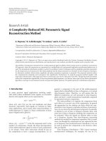
Figure 1: Illustration of the SR reconstruction of all frames in the
video.
algorithm to solve the nonlinear TV-based SR reconstruc-
tion model using fixed-point and preconditioning methods.
Preconditioned conjugate gradient methods with factorized
banded inverse preconditioners are employed in the itera-
tions. Experimental results show that our method is more ef-
ficient than the gradient descent method. Secondly, we com-
bine image inpainting and SR reconstruction together to ob-

tain an HR image from a sequence of LR images. We con-
sider that there exist some missing and/or corrupted pix-
els in LR images. The filling-in of such missing and/or cor-
rupted pixels in an image is called image inpainting [32]. By
putting missing and/or corrupted pixels in the image obser-
vation model, the proposed algorithm can perform image in-
painting and SR reconstruction simultaneously. Experimen-
tal results validate that it is more robust than the method
of conducting image inpainting and SR reconstruction sepa-
rately. Thirdly, while our algorithm is developed for the cases
where raw uncompressed video data (such as a webcam di-
rectly linked to a host computer) is used, it can be applied to
the MPEG compressed video. Simulation results show that
the proposed algorithm is also capable of SR reconstruction
with the compressed artifacts in the video.
It is noted that this paper aims to reconstruct an HR
frame from several LR frames in the video. Using the pro-
posed algorithm, all the frames in the video can be SR re-
constructed in such a way [33]: for a given frame, a “sliding
window” determines the set of LR frames to be processed to
produce the output. The window is moved forward to pro-
duce successive SR frames in the output sequence. An illus-
tration of this procedure is given in Figure 1.
The outline of this paper is as follows. In Section 2,
we present the image observation model of the SR prob-
lem. The motion estimation methods used in this paper
are described in Section 3.InSection 4, we present the TV
regularization-based reconstruction algorithm. Experimen-
tal results are provided in Section 5. Finally, concluding re-
marks are given in Section 6.

2. IMAGE OBSERVATION MODEL
In SR image reconstruction, it is necessary to select a frame
from the sequence as the referenced one. The image ob-
servation model is to relate the desired referenced HR im-
age to all the observed LR images. Typically, the imaging
process involves warping, followed by blurring and down-
sampling to generate LR images from the HR image. Let
the underlying HR image be denoted in the vector form by
z
= [z
1
, z
2
, , z
L
1
N
1
×L
2
N
2
]
T
,whereL
1
N
1
× L
2

N
2
is the HR
image size. Letting L
1
and L
2
denote the down-sampling fac-
tors in the horizontal and vertical directions, respectively,
each observed LR image has the size N
1
× N
2
. T hus, the LR
image can be represented as y
k
= [y
k,1
, y
k,2
, , y
k,N
1
×N
2
]
T
,
where k
= 1, 2, , P,withP being the number of LR im-

ages. Assuming that each observed image is contaminated by
additive noise, the observation model can be represented as
[17, 34, 35]
y
k
= DB
k
M
k
z + n
k
,(1)
where M
k
is the motion (shift, rotation, zooming, etc.) ma-
trix with the size of L
1
N
1
L
2
N
2
× L
1
N
1
L
2
N

2
, B
k
represents the
blur (sensor blur, motion blur, atmosphere blur, etc.) matrix
also of size L
1
N
1
L
2
N
2
× L
1
N
1
L
2
N
2
, D is an N
1
N
2
× L
1
N
1
L

2
N
2
down-sampling matrix, and n
k
represents the N
1
N
2
×1noise
vector .
In fact, in an unreferenced frame, there often exists oc-
clusions that cannot be observed in the referenced frame.
Obviously, these occlusions should be excluded in the SR
reconstruction. Furthermore, there are also missing and/or
corrupted pixels in the observed images in some cases. In
order to deal with the occlusion problem and perform the
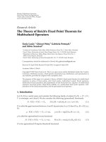
image inpainting along with the SR, the observation model
(1) should be expanded. We use the term unobservable to de-
scribe all the occluded, missing, and corrupted pixels, and ob-
servable to describe the other pixels. The unobservable pixels
can be excluded by modifying the observation model as
y
obs
k
= O
k

DB
k

M
k
z + n
k

,(2)
where O
k
is an operator cropping the observable pixels from
y
k
,andy
obs
k
is the cropped result. This model provides the
possibility to deal with the occlusion problem and to con-
duct simultaneous inpainting and SR. A block diagram cor-
responding to the degradation process of this model is illus-
trated in Figure 2.
3. MOTION ESTIMATION METHODS
Motion estimation/registration plays a critical role in SR re-
construction. In general, the subpixel motions between the
referenced frame and the unreferenced frames can be mod-
eled and estimated by a parameter model, or they may be
scene dependent and have to be estimated for every point
[36]. This section introduces the motion estimation meth-
ods employed in this paper. For a comparative analysis of the
subpixel motion estimation methods in SR reconstruction,
please refer to [37].
3.1. Parameter model-based motion estimation

Typically, if the objects in the scene remain stationary while
the camera moves, the motions of all points often can be
modeled by a parametric model. Generally, the relationship
between the observed kth and lth frames can be expressed by
y
k

x
u,
x
v

= y

(l,θ)
k

x
u,
x
v

+ ε
l,k

x
u,
x
v


,(3)
Michael K. Ng et al. 3
M
k
B
k
D
n
k
O
k
Figure 2: Block diagram illustration of the observation model (2), where the far left is the desired high-resolution image, and the far right is
the observed image.
where (x
u
, x
v
) denotes the pixel site, y
k
(x
u,
x
v
) is a pixel in
frame k, θ is the vector containing the corresponding motion
parameters, y

(l,θ)
k
(x

u,
x
v
) is the predicted pixel of y
k
(x
u,
x
v
)
from frame l using parameter vector θ,andε
l,k
(x
u,
x
v
)denotes
the model error. In the literature, the six-par ameter a ffine
model and eight-parameter perspective model are widely
used.Hereweconcentrateontheaffine model, in which
y

(l,θ)
k
(x
u,
x
v
) can be expressed as
y


(l,θ)
k

x
u,
x
v

=
y
l

a
0
+ a
1
x
u
+ a
2
x
v
, b
0
+ b
1
x
u
+ b

2
x
v

. (4)
In this model, θ
= (a
0
, a
1
, a
2
, b
0
, b
1
, b
2
)
T
contains six geo-
metric model parameters. To solve θ, we can employ the least
square criterion, which has the following minimization cost
function:
E(θ)
=


y
k

− y

(l,θ)
k


2
2
. (5)
Using the Gaussian-Newton method, the six affine parame-
ters can be iterativ ely solv ed by
Δθ
=

J
n

T
J
n

−1

−

J
n

T
r

n

,
θ
n+1
= θ
n
+ Δθ.
(6)
Here, n is the iteration number, Δθ denotes the corrections of
the models parameters, r
n
is the residual vector that is equal
to y
k
− y

(l,θ
n
)
k
,andJ
n
= ∂r
n
/∂θ
n
denotes the gradient matrix
of r
n

.
3.2. Optical flow-based motion estimation
In many videos, the scene may consist of independently mov-
ing objects. In this case, the motions cannot be modeled by a
parametric model, but we can use optical flow-based meth-
ods to estimate the motions of all points. Here we intro-
duce a simple MAP motion estimation method. Let us de-
note m
= (m
u,
m
v
) as a 2D motion field which describes the
motions of all points between the observed frames y
k
and
y
l
with m
u
and m
v
being the horizontal and vertical fields,
respectively, and y

(l,m)
k
is the predicted version of y
k
from

frame l using the motion field m, the MAP motion estima-
tion method has the following minimization function [38]:
E(m)
=


y
k
− y

(l,m)
k


2
2
+ λ
1
U(m), (7)
where U(m) describes prior information of the motion filed
m,andλ
1
is the regularization parameter. In this paper, we
choose U(m) as a Laplacian smoothness constraint consist-
ing of the terms
Qm
u

2
+ Qm

v

2
,whereQ is a 2D Lapla-
cian operator. Using steepest descent method, we can itera-
tively solve the motion vector field by
m
n+1
u
= m
n
u
+ α

∂y

(l,m)
k
∂m
u

y
k
− y

(l,m)
k

−
λ

1
Q
T
Qm
u

,
m
n+1
v
= m
n
v
+ α

∂y

(l,m)
k
∂m
v

y
k
− y

(l,m)
k

− λ

1
Q
T
Qm
v

,
(8)
where n again is the iteration number, and α is the step size.
Thederivativeintheaboveequationiscomputedonapixel-
by-pixel basis, given by
∂y

(l,m)
k

x
u
, x
v

∂m
u
=
y
l

x
u
+ m

u
+1,x
v

−
y
l

x
u
+ m
u
− 1,x
v

2
,
∂y

(l,m)
k

x
u
, x
v

∂m
v
=

y
l

x
u
, x
v
+ m
v
+1

−
y
l

x
u
, x
v
+ m
v
− 1

2
.
(9)
Whether using parameter-based model or using opti-
cal flow-based model, the unobservable pixels defined in
Section 2 should be excluded in the SR reconstruction.
Sometimes their positions are known, such as when some

pixels (the corresponding sensor array elements) are not
functional. However, in many cases when they are not known
in advance, a simple way to determine them is to make a
threshold judgment on the warping error of each pixel by


y
k
− y

(l,θ)
k


<d (10)
or


y
k
− y

(l,m)
k


<d (11)
depending on which motion estimation model is used. Here,
d is a scalar threshold.
4. TOTAL VARIATION-BASED

RECONSTRUCTION ALGORITHM
4.1. TV-based SR model
In most situations, the problem of SR is an ill-posed inverse
problem because the information contained in the observed
LR images is not sufficient to solve the HR image. In order
to obtain more desirable SR results, the ill-posed problem
4 EURASIP Journal on Advances in Signal Processing
should be stabilized to become well-posed. Traditionally, reg-
ularization has been described from both the algebraic and
statistical perspectives [39]. Using regular ization techniques,
the desired HR image can be solved by
z = arg min


k


yk
obs
− O
k
DBM
k
z


2
+ λ
2
Γ(z)


, (12)
where

k
y
obs
k
− O
k
DBM
k
z
2
is the data fidelity term, Γ(z)
denotes the regularization term, and λ
2
is the regularization
parameter. It is noted that we assume all the images have the
same blurring function, so the matrix B
k
has been substi-
tuted by B.
For the regularization term, Tikhonov and Gauss-
Markov types are commonly employed. A common criti-
cism to these regularization methods is that the sharp edges
and detailed information in the estimates tend to be overly
smoothed. When there is considerable motion error, noise,
or blurr ing in the system, the problem is magnified. To ef-
fectively preserve the edge and detailed information in the

image, some edge-preserving regularization should be em-
ployed in the SR reconstruction.
An effective total variation (TV) regularization was first
proposed by Rudin et al. [40] in image processing field. The
standard TV norm looks like
Γ(z)
=

Ω
|∇z| dxdy =

Ω

|∇z|
2
dx dy, (13)
where Ω is the 2-dimensional image space. It is noted that the
above expression is not differentiable when
∇z = 0. Hence, a
more general expression can be obtained by slightly revising
(13), given as
Γ(z)
=

Ω

|∇z|
2
+ βdxdy. (14)
Here, β is a small positive parameter which ensures differen-

tiability. Thus the discrete expression is written as
Γ(z)
=∇z
TV
=

i

j



∇
z
1
i, j


2
+


∇
z
2
i, j


2
+ β, (15)

where
∇z
1
i,j
= z[i+1, j]−z[i, j]and∇z
2
i, j
= z[i, j+1]−z[i, j].
The TV regularization was first proposed for image denoising
[40]. Because of its robustness, it has been applied to image
deblurring [41], image interpolation [42], image inpainting
[32],andSRimagereconstruction[24, 28–31].
In [43], the authors used the l
1
regularization
Γ(z)
=

i

j



∇
z
1
i, j



+


∇
z
2
i, j



(16)
to approximate the TV regularization. In [24, 31], Farsiu et
al. proposed the so-called bilateral TV (BTV) regularization
in SR image reconstruction. The BTV regularization looks
like
Γ(z)
=
P

l=−P
P

m=0
α
|m|+|l|


z − S
l
x

S
m
y
z


1
, (17)
where operators S
l
x
and S
m
y
shift z by l and m pixels in hori-
zontal and vertical directions, respectively. The scalar weight
α,0<α<1, is applied to g ive a spatially decaying effect to
the summation of the regularization terms [31]. The authors
also pointed out that the l
1
regularization can be regarded as
a special case the BTV regularization.
We call these two regularizations (l
1
and BTV) as TV-
related regularizations in this paper. However, the distinction
between these two regularizations and the standard TV reg-
ularization should b e kept in mind. Bioucas-Dias et al. [44]
have demonstrated that TV regularization can lead to better
results than the l

1
regularization in image restoration. There-
fore, we employ the standard TV regularization (15) in this
paper. By substituting (15)in(12), the following minimiza-
tion function can be obtained:
z = arg min


k


y
obs
k
− O
k
DBM
k
z


2
+ λ
2
∇z
TV

.
(18)
4.2. Efficient optimization method

We should note that although the TV regularization has been
applied to SR image reconstruction in [24, 28–31], most of
these methods use the gradient descent method to solve the
desired HR image. In this section, we introduce a more ef-
ficient and reliable algorithm for the optimization problem
(18).
The Euler-Lagrange equation for the energy function in
(18) is given by the following nonlinear system:
∇E(z) =

k
M
T
k
B
T
D
T
O
T
k

O
k
DBM
k
z − y
obs
k


− λ
2
L
z
z = 0,
(19)
where L
z
is the matrix form of a central difference approxi-
mation of the differential operator
∇·(∇/

|∇z|
2
+ β)with
∇· being the divergence operator. Using the gradient descent
method, the HR image z is solved by
z
n+1
= z
n
− dt∇E

z
n

, (20)
where n is the iteration number, and dt > 0 is the time step
parameter restricted by stability conditions (i.e., dt has to be
small enough so that the scheme is stable). The drawback of

this gradient descent method is that it is difficult to choose
time steps for both efficiency and reliability [43].
One of the most popular strategies to solve the nonlinear
problem in (19) is the lagged diffusivity fixed point iteration
introduced in [45, 46]. This method consists in linearizing
the nonlinear differential term by lagging the diffusion coef-
ficient 1/

|∇z|
2
+ β one iteration behind. Thus z
n+1
is ob-
tained as the solution to the linear equation


k=1
M
T
k
B
T
D
T
O
T
k
O
k
DBM

k
− λL
n
z

z
n+1
=

k=1
M
T
k
B
T
D
T
O
T
k
y
obs
k
.
(21)
Michael K. Ng et al. 5
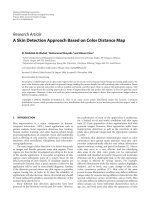
(a) (b)
Figure 3: The 24th frame in the “Foreman” sequence. (a) The original 352 × 288 image and (b) the extracted 320 × 256 image.
It has been showed in [45] that the method is monotoni-
cally convergent. To solve the above linear equation, any lin-

ear optimization solution can be employed. Generally, the
preconditioned conjugate gradient (PCG) method is desir-
able. To suit the specific mat rix structures in image restora-
tion and reconstruction, several preconditioners have been
proposed [47–51]. An efficient way to solving the matrix
equations in h igh-resolution image reconstruction is to ap-
ply the factorized sparse inverse preconditioner (FSIP) [50].
Let A be a symmetric positive definite matrix, and let its
Cholesky factorization be A
= GG
T
. The idea of FSIP is to
find the lower triangular matrix L with sparsity pattern S
such that
I − GL
F
(22)
is minimized, where
·
F
denotes the Frobenius norm.
Kolotilina and Yeremin [50] showed that L can be obtained
by the following algorithm.
Step 1. Compute

L with sparse pattern S such that [

LA]
x,y
=

δ
x,y
,(x, y) ∈ S.
Step 2. Let

D = (diag(

L))
−1
and L =

D
1/2

L.
According to this algorithm, m small linear systems need
to be solved, where m is the number of rows in the matrix
A. These systems can be solved in parallel. Thus the above
algorithm is also well suited for modern parallel computing.
Motivated by the FSIP preconditioner, we consider the
factorized banded inverse preconditioner (FBIP) [47]which
is a special type of FSIP. The main idea of FBIP is to approxi-
mate the Cholesky factor of the coefficient matrix by banded
lower triangular matrices. The following theorem has been
proved in [47].
Let T be a Hermitian Toeplitz matrix, and let B
= T or
B
= I + T
T

DT with D be a positive diagonal matrix. Denote
the kth diagonal of T by t
k
. Assume the diagonals of T satisfy


t
k


≤
ce
−γ|k|
(23)
for some c>0andγ>0, or


t
k


≤
c

|k| +1

−s
(24)
for some c>0ands>3/2. Then for any given ε>0, there
exists a p


> 0 such that for all p>p

,


L
p
− C
−1


≤
ε, (25)
where L
p
denotes the FBIP of B with the lower bandwidth
p,andC is the Cholesky factor of B. This theorem indicates
that if the Toeplitz matrix T has certain off-diagonal decay
property, then the FBIPs of B wil l be good approximation of
B
−1
. Here we should note that even though the system matrix
in (21) is not exactly in the Toeplitz form or in I+T
T
DT form,
our experimental results indicate that the FBIP algorithm is
still very efficient for this problem.
5. SIMULATION RESULTS
We tested the proposed TV-based SR reconstruction al-

gorithm using a raw “Foreman” sequence and a realistic
MPEG4 “Bulletin” sequence. The algorithm using Lapla-
cian regularization (where the regularization term is
Qz
2
,
with Q being the 2-dimensional Laplacian operator) was
also tested to make a comparative analysis. It is noted that
the Laplacian regularization generally has stronger constraint
on the image than the TV regularization because it is a
square term and not extracted like the TV regularization, so
it should require a smaller regularization parameter. In fact,
we should respectively choose the optimal regularization pa-
rameters for the two different regularizations for a reason-
able comparison. With this in mind, we tried a series of reg-
ularization parameters for the two regularizations in all the
experiments. Furthermore, we also compared our proposed
algorithm to other TV or TV-related algorithms in the “Fore-
man” experiments.
5.1. The “Foreman” sequence
We first tested the popular “Foreman” sequence with a 352
×
288 CIF format. One frame (the 24th) of this sequence is
shown in Figure 3(a). It is seen that there are two dark re-
gions, respectively, at the left and lower boundaries, and
that there is also a labeled region around the top left cor-
ner. To make reliable quantitative analysis, most of the pro-
cessing was restricted to the central 320
× 256 pixel region.
The 320

× 256 extracted version of Figure 3(a) is shown in
6 EURASIP Journal on Advances in Signal Processing
1E − 06 3E − 05 1E − 03 3E − 02
λ
35
37
39
41
43
45
47
49
PSNR (dB)
TV
Laplacian
(a)
1E − 06 3E − 05 1E − 03 3E − 02 1E +00
λ
25
30
35
40
PSNR (dB)
TV
Laplacian
(b)
3E − 02 1E − 01 4E − 01 2E +00 7E +00
λ
25
27

29
31
33
35
PSNR (dB)
TV
Laplacian
(c)
1E − 06 3E − 05 1E − 03 3E − 02 1E +00
λ
20
25
30
35
40
45
PSNR (dB)
TV
Laplacian
(d)
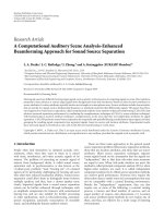
Figure 4: PSNR values versus the regularization parameter in the synthetic “Foreman” experiments: (a) the “motion only” case, (b) the
“blurring” case, (c) the “noise” case, and (d) the “missing” case.
Figure 3(b). The following peak signal-to-noise ratio (PSNR)
was employed as the quantitative measure:
PSNR
= 10 log
10

255
2

∗ L
1
N
1
L
2
N
2
z − z
2

, (26)
where L
1
N
1
L
2
N
2
is the total number of pixels in the HR im-
age, and
z and z represent the reconstructed HR image and
the original image, respectively.
5.1.1. Synthetic simulations
To show the feature and advantage of the TV-based recon-
struction algorithm more sufficiently, we first implemented
the synthetic experiments in which the LR images are simu-
lated from a single frame of the “Foreman” sequence, frame
24 (the extrac ted 320

× 256 version). Using observation
model (2), we simulated the LR frames in four different
ways: (1) the “motion only” case, in which the original frame
was first warped and then the warped versions were down-
sampled to obtain the LR frames; (2) the “blurring” case,
in which the original frame was first blurred with a 5
× 5
Gaussian kernel before the warping; (3) the “noise” case, in
which the LR frames obtained in the “motion only” case were
then contaminated by Gaussian noise with 65.025 variance;
and (4) the “missing” case, in which some missing regions
were assumed to exist at the same positions of all the LR
frames. For each case, the down-sampling factor was two,
and four LR images were simulated using global translational
motion model. PSNR values against the regularization pa-
rameter λ
2
in the four cases are demonstrated in Figures
4(a)–4(d), respectively. The SR reconstruction results are re-
spectively shown in Figures 5–8.
In the “motion only” case, the best PSNR result using
Laplacian regularization is 46.162 dB with λ
2
= 0.000256 and
that of TV is 47.360 dB w ith λ
2
= 0.016384 (see Figure 4(a)).
As expected, the use of TV regularization provided a higher
PSNR value. However, since the motions were accurately
Michael K. Ng et al. 7

(a) (b) (c)
Figure 5: Experimental results in the synthetic “motion only” case. (a) LR frame, (b) Laplacian SR result with λ
2
= 0.000256 and (c) TV SR
result with λ
2
= 0.016384.
(a) (b) (c)
Figure 6: Experimental results in the synthetic “blurring” case. (a) LR frame, (b) Laplacian SR result with λ
2
= 0.0001 and (c) TV SR result
with λ
2
= 0.008192.
known and there is no noise, blurring, or missing pixel in
the image, the result using Laplacian regularization also has
high quality. As a result, Figures 5(b) and 5(c) are almost in-
distinguishable visually.
From Figures 4(b) and 6, we can see the advantage of the
TV-based reconstruction algorithm is much more obvious in
the “blurring” case. Figure 6(b) is the Laplacian result with
the best PSNR of 34.845 dB (λ
2
= 0.00256), and Figure 6(c)
shows the TV result with the best PSNR of 37.663 dB (λ
2
=
0.008192). Visually, the use of Laplacian regular ization leads
to some artifacts in the reconstructed image. TV regulariza-
tion, however, does well.

In the “noise” case, the best PSNR value for the Laplacian
regularization is 32.968 dB with the regularization parameter
being 0.1024. Using TV regularization, however, we obtained
a best PSNR value of 34.987 dB when the regularization pa-
rameter is equal to 3.2768. The images corresponding to the
best PSNR values are shown in Figures 7(b) and 7(c),respec-
tively. Both images are still noisy to some extent although
they have the highest PSNR values, and Figure 7(b) is more
obvious. To further smooth the noise, larger regularization
parameters should be chosen. Figure 7(d) is the Laplacian re-
sult with λ
2
= 3.2768, and Figure 7(e) is the TV result with
λ
2
= 6.5536. The PSNRs of these two images are 29.797 dB
(Laplacian) versus 34.459 dB (TV). The TV-based algorithm
is preferable again because it can provide simultaneous de-
noising and edge preservation.
Figures 4(d) and 8 show the “missing” case. This is a
typical example of the simultaneous image inpainting and
SR. The best PSNR values for Laplacian and TV are, re-
spectively, 37.315 dB (λ
2
= 0.008192) and 41.400 dB (λ
2
=
0.016384). The corresponding results are shown in Figures
8(b) and 8(c), respectively. We also give the results using
larger regularization parameters in Figure 8(d) (Laplacian,

λ
2
= 0.065536, PSNR = 35.282 dB) and Figure 8(e) (TV,
λ
2
= 0.26214, PSNR = 40.176 dB), respectively. These two
images have better visual quality in the missing regions than
their counterparts, Figures 8(b) and 8(c).Wecanclearlysee
that the missing regions can be desirably inpainted using the
TV-based algorithm. However, the Laplacian regularization
does not work well. Figure 8(f) shows the reconstruction re-
sult using TV regularization (λ
2
= 0.26214) by conducting
image inpainting and SR separately. The missing regions can-
not be inpainted as good as that in the simultaneous process
case. The PSNR of Figure 8(f) is 35.003.
5.1.2. Nonsynthetic simulations
In the nonsynthetic experiments, the LR images used in the
SR reconstruction are produced from the corresponding HR
8 EURASIP Journal on Advances in Signal Processing
(a) (b)
(c) (d) (e)
Figure 7: Experimental results in the synthetic “noise” case. (a) LR frame, (b) Laplacian SR result with λ
2
= 0.1024, (c) TV SR result with
λ
2
= 3.2768, (d) Laplacian SR result with λ
2

= 3.2768 and (e) TV SR result w ith λ
2
= 6.5536.
(a) (b) (c)
(d) (e) (f)
Figure 8: Experimental results in the synthetic “missing” case. (a) LR frame, (b) Laplacian simultaneous inpainting and SR result with
λ
2
= 0.008192, (c) TV simultaneous inpainting and SR result with λ
2
= 0.016384, (d) Laplacian simultaneous inpainting and SR result with
λ
2
= 0.065536, (e) TV simultaneous inpainting and SR result with λ
2
= 0.26214, and (f) TV result conducting inpainting and SR separately
with λ
2
= 0.26214.
Michael K. Ng et al. 9
(a) (b)
Figure 9: Motion estimates of frame 22 (a) and frame 25 (b) in the nonsynthetic “Foreman” experiment.
(a) (b)
Figure 10: The unobservable pixels of frame 22 (a) and frame 25 (b) in the nonsynthetic “Foreman” experiment.
frames in the video with a downsampling factor of two. Here,
we again demonstrate the reconstruction results of frame 24.
Frames 22, 23, 25, and 26 were used as the unreferenced ones.
We first tested the “motion only” case. It is noted that the mo-
tions are unknown and should be estimated in the nonsyn-
thetic cases. We employed the motion estimation method in-

troduced in Section 3.2,withλ
1
= 10000 and α = 10
−6
.The
motion estimates of frames 22 and 25 are shown in Figure 9
as illustrations. After the motion estimation, (11)wasused
to determine the unobser vable pixels, and the threshold d
was chosen to be 6. Figures 10(a) and 10(b) illustrate the
unobservable pixels of frame 22 and 25, respectively. Recon-
struction methods using Laplacian regularization and TV
regularization were respectively implemented. PSNR value
against the regularization parameter λ
2
is demonstrated in
Figure 11(a). The best PSNR result with Laplacian regular-
ization is 36.185 dB with λ
2
= 0.008, and that of TV is
37.336 dB with λ
2
= 0.512. Again, the TV performs better
than Laplacian quantitatively. Furthermore, unlike the syn-
thetic “motion only” case, the advantage of the TV-based re-
construction is also visually obvious. The Laplacian result is
shown in Figure 12(b), from which we can find that the sharp
edges are obviously damaged due to the inevitable motion es-
timation errors. In the TV result shown in Figure 12(c),how-
ever, these edges are effectively preserved.
We also show the nonsynthetic “noise” case in which

random Gaussian noise with 32.5125 variance was added to
the down-sampled images. One of the noisy LR frames is
shown in Figure 13(a). Figure 11(b) shows the curves of the
PSNR value versus the regularization parameter. The best
PSNR values are, respectively, 32.040 dB and 33.851 dB for
the Laplacian and TV. The corresponding reconstructed im-
ages are illustrated in Figures 13(b) and 13(c), and the results
with larger regularization parameters which have better vi-
sual quality regarding the noise are shown in Figures 13(d)
and 13(e), respectively. By comparisons, we see that the TV-
based reconstruction algorithm outperforms the Laplacian-
based algorithm in terms of both the visual evaluation and
quantitative assessment again.
In order to demonstrate the efficacy of the proposed
algorithm, we reconstructed the first 60 frames in the
“Foreman” sequence and then combined them together
to video format. The regularization parameters for all
frames were the same, and the parameters used can pro-
vide almost the best visual equality in each case. The SR
videos with WMV format can be found at the website
/>noted that the original frames with size of 352
×288 were used
now. We also tried to deal w ith the missing and labeled re-
gions in the original video frames in the “motion only” case.
Actually, it is impossible to perfect ly inpaint these regions
because their areas are too large and they are located at the
boundaries of the image. However, our experiment indicates
that the TV-based reconstruction algorithm has the efficacy
to provide a more desirable result as seen in Figure 14.
5.1.3. Comparison to other TV methods

In Sections 5.1.1 and 5.1.2, we compared the proposed TV
regularization-based algorithm (FBIP TV algorithm) to the
10 EURASIP Journal on Advances in Signal Processing
1E − 03 8E − 03 6E − 02 5E − 01 4E +00
λ
30
32
34
36
38
PSNR (dB)
TV
Laplacian
(a)
1E − 03 8E − 03 6E − 02 5E − 01 4E +00
λ
25
27
29
31
33
35
PSNR (dB)
TV
Laplacian
(b)
Figure 11: PSNR values versus the regularization parameter in the nonsynthetic “Foreman” experiments: (a) the “motion only” case, and
(b) the “noise” case.
(a) (b) (c)
Figure 12: Experimental results in the nonsynthetic “motion only” case. (a) LR frame, (b) Laplacian SR result with λ = 0.008 and (c) TV

SR result with λ
= 0.512.
Laplacian regularization-based algorithm from the reliabil-
ity perspective. In this subsection, we compare it to other
TV-based algorithms which employ gradient descent (GD)
method in terms of both efficiency and reliability. In the ex-
periments, the iteration was terminated when the relative
gradient norm d
=∇E(z
n
)/∇E(z
0
) was smaller or it-
eration number N was larger than some thresholds. We have
mentioned that the drawback of the GD method is that it is
difficult to choose time step dt for both efficiency and relia-
bility. Therefore, we repeated several parameters in each case
of the experiments. Here we show the reconstruction results
using almost the optimal step parameters. We also tested the
effect of parameter β in (14).
Table 1 shows the synthetic “noise-free” case with the
full 4 frames being used. Since the problem is almost over-
determined in this case, we believe most algorithms can be
employed from the reliability perspective. From Table 1,we
can see the PSNR value of the result using FBIP TV algorithm
is even lower than that of the GD TV algorithm. But the GD
TV algorithm is not stable when dt increases to 1.0. From the
efficiency perspective, the FBIP TV algorithm is faster than
the GD TV and GD BTV algorithms. We also can see that
a relatively larger parameter β leads to much faster conver-

gence speed for the FBIP TV algorithm, but the efficiency ef-
fect of β to the GD TV algorithm is negligible. The reliability
of both FBIP TV and GD TV algorithms is not sensitive to
the choice of β.
Table 2 shows the synthetic “noise-free” case with only
2 frames being used. In this case, the problem is strongly
under-determined. We can see that the efficiency advantage
of the FBIP TV algorithm is very obvious. The FBIP TV algo-
rithm also leads to higher PSNR values than the GD TV and
BTV algorithms.
Table 3 shows the synthetic “missing” case. The FBIP TV
algorithm is still very efficient when there are missing regions
in the image. However, the convergence speed of the GD TV
and GD BTV are extremely slow. Larger regular ization or
larger parameter P (in BTV) can speed up the processing,
but cannot ensure the optimal solution.
Figure 15 shows the convergence performance in the
nonsynthetic “noisy-free” c ase. Figure 15(a) illustrates the
evolution of the gradient norm-based convergence condition
Michael K. Ng et al. 11
(a) (b)
(c) (d) (e)
Figure 13: Experimental results in the nonsynthetic “noise” case. (a) LR frame, (b) Laplacian SR result with λ = 0.128, (c) TV SR result with
λ
= 2.048, (d) Laplacian SR result with λ = 2.048, and (e) TV SR result with λ = 4.096.
(a) (b)
Figure 14: Reconstruction results of the “Foreman” with the original size. (a) Laplacian regularization and (b) TV regularization.
∇E(z
n
)/∇E(z

0
) against the computational time, and
Figure 15(b) is the demonstration of PSNR value versus
the computational time. From both the gradient norm and
PSNR convergence c riteria, the FBIP TV algorithm greatly
outperforms the GD TV algorithm and GD BTV algorithm.
It is not only very efficient, but also very stable. In all the pre-
vious experiments, the di fferential operator in (19) was ap-
proximated by central difference for both GD TV and FBIP
TV algorithms. In this case, we also tested the backward dif-
ference approximation for the GD TV algorithm (not that
backward difference cannot be used for the FBIP TV algo-
rithm because the corresponding system matrix is not sym-
metric and positive). The l
1
regularization was also tested.
Table 4 shows the PSNR values of different algorithms. Here
we note that the selected termination conditions can ensure
the optimal results for all the regularizations with the cur-
rent parameter settings. It is seen that the proposed FBIP TV
algorithm outperforms all other algorithms.
5.2. The “bulletin” sequence
In this experiment, we show the SR reconstruction of a “bul-
letin” sequence which was obtained from a consumer-level
digital video camera. One frame of this sequence is shown in
Figure 16. Although the original frame size is 640
×480 pixels,
our processing was restricted to a typical 450
× 80 pixel, as
shown in (boxed in dashed) in Figure 16.

Here we used seven extracted 450
× 80 images to pro-
duce a 900
× 160 SR image. Since there is no independently
12 EURASIP Journal on Advances in Signal Processing
Table 1: Compar ison with GD TV and BTV algorithms in the synthetic “noise-free” case (4 frames).
λ dt β Termination Time (s) PSNR (dB)
FBIP TV 0.016
— 10
−5
d = 5 × 10
−4
16.063 47.360
— 10
−1
d = 5 × 10
−4
11.422 47.426
GD TV 0.016
0.2
10
−5
d = 5 × 10
−4
73.031 47.707
10
−1
d = 5 × 10
−4
70.312 47.709

0.6
10
−5
d = 5 × 10
−4
24.531 47.722
10
−1
d = 5 × 10
−4
23.141 47.709
1.0
10
−5
d = 5 × 10
−4
15.063 47.733
10
−1
d = 5 × 10
−4
14.530 47.712
10
−5
N = 2000 303.406 47.274
GD BTV (P = 1) 0.007
0.6 — d = 5 × 10
−4
41.828 47.385
1.0 — d = 5 × 10

−4
34.140 47.265
Table 2: Compar ison with GD TV and BTV algorithms in the synthetic “noise-free” case (2 frames).
λ dt β Termination Time (s) PSNR (dB)
FBIP TV 0.016
— 10
−5
d = 1 × 10
−3
18.140 40.201
— 10
−1
d = 1 × 10
−3
13.718 40.166
GD TV 0.016 0.5 10
−5
d = 2 × 10
−3
93.734 39.038
GD BTV (P = 1) 0.007 0.5 — d = 2 × 10
−3
179.093 38.623
Table 3: Comparison with GD TV and BTV algorithms in the synthetic “missing” case (4 frames).
λ dt β Termination Time (s) PSNR (dB)
FBIP TV 0.016
— 10
−5
d = 1 × 10
−5

33.875 41.373
— 10
−1
d = 1 × 10
−5
20.062 41.239
GD TV
0.016 1.0 10
−5
N = 3000 380.087 17.410
0.1 1.0
10
−5
N = 3000 384.890 23.968
10
−5
N = 6000 762.343 28.324
10
−5
N = 9000 1139.56 32.577
BTV (P = 1) 0.1 1.0 —
N = 3000 335.187 26.883
N = 6000 670.343 33.925
N = 9000 1018.43 39.460
N = 10000 1135.72 39.460
GD BTV (P = 3) 0.1 1.0 —
N = 1000 376.047 30.170
N = 2000 749.141 38.839
N = 3000 1191.70 38.861
Table 4: Compar ison with GD TV and BTV algorithms in the nonsynthetic “noise-free” case (5 frames).

λ dt β Termination PSNR (dB)
FBIP TV(Central) 0.512 — 10
−5
d = 1 × 10
−3
37.336
GD TV (Central)
0.512 0.05 10
−5
N = 1000 37.206
GD TV (Backward)
0.512 0.05 10
−5
N = 1000 37.084
GD L1
0.2 0.05 — N = 1000 36.576
GD BTV (P
= 1) 0.2 0.05 — N = 1000 36.854
GD BTV (P
= 2) 0.2 0.05 — N = 1000 36.875
GD BTV (P
= 3) 0.1 0.05 — N = 1000 36.873
Michael K. Ng et al. 13
0 20 40 60 80 100 120 140 160 180
Time (s)
10
−4
10
−3
10

−2
10
−1
10
0
∇E(z
n
)/∇E(z
0
)
FBIP TV (β = 0.1)
GD TV (dt
= 0.05)
GD BTV (dt
= 0.05)
GD BTV (dt
= 0.1)
(a)
0 20 40 60 80 100 120 140 160 180
Time (s)
31
32
33
34
35
36
37
38
PSNR (dB)
FBIP TV (β = 0.1)

GD TV (dt
= 0.05)
GD BTV (dt
= 0.05)
GD BTV (dt
= 0.1)
(b)
Figure 15: Convergence performance of different algorithms, (a) measured by gradient norm, (b) measured by PSNR value.
Figure 16: One 640 × 480 frame in the “bulletin” video. The region
boxed in dashed is the interest.
moving object in the scene, the motions between the refer-
enced image and the unreferenced images can be estimated
by the affine parameter model introduced in Section 3.1.
Figure 17(a) shows one of the extracted images. It is observed
that there are obvious artifacts in most parts of this image.
These artifacts mainly come from the compression process of
the MPEG video. Figure 17(b) is the SR reconstruction result
using Laplacian regularization with a relatively smaller regu-
larization parameter 0.001. The characters in the image look
clearer, but the compression artifact is aggravated. To solve
this problem, higher regularization parameter should be cho-
sen. In our experiment, we found the artifact problem could
not be solved until we increase the regularization parame-
ter to 0.5. The reconstructed image is shown in Figure 17(c).
Although the artifacts are suppressed, the characters are too
smooth. However, the TV-based reconstruction algorithm
can effectively solve this tradeoff. Figure 17(d) shows the TV
reconstruction result with λ
2
= 5.0. Its overall visual qual-

ity is much better than that of Figures 17(a)–17(c). Detailed
cropped regions from Figures 17(a)–17(d) are, respectively,
demonstrated in Figures 18(a)–18(d),fromwhichwecansee
the advantage of the TV-based SR reconstruction more easily.
It is noted that we did not consider the compression
and decompression processes in the reconstruction model
although the inputs of this experiment are the decoded
frames from the MPEG video. But even in this case, we ob-
tained desirable super-resolved result using the TV-based SR
algorithm. If the compression and decompression processes
also were included in the SR model such as the methods in
[26, 27], the result should be better.
6. CONCLUSIONS
The SR reconstruction of digital video becomes difficult
when there is blurring, noise, missing regions, compression
artifacts, or inevitable motion estimation errors in the sys-
tem. To address these challenges, we have proposed a robust
and efficient TV-based SR algorithm in this paper. The pro-
posed algorithm has been tested in different cases. Experi-
mental results show that i t performs quite well in terms of
both robustness and efficiency. Nevertheless, further work
can potentially improve upon the proposed algorithm, such
as the inclusion of the compression process in the reconstruc-
tion model and the consideration of TV regularization in the
motion estimation step. The adaptive determination of the
number of the input frames in the SR reconstruction is also
another possibility.
14 EURASIP Journal on Advances in Signal Processing
(a) (b)
(c) (d)

Figure 17: SR reconstruction results of the “bulletin” sequence. (a) LR frame, (b) Laplacian SR result with λ
2
= 0.001, (c) Laplacian SR
result with λ
2
= 0.5, and (d) TV SR result with λ
2
= 5.0.
(a) (b) (c) (d)
Figure 18: (a)–(d) Detail regions cropped from Figures 17(a)–17(d).
ACKNOWLEDGMENTS
Research supported in part by RGC 7035/04P and 7035/05P,
and HKBU FRGs. H. Shen would like to thank M. K. Ng
for his hospitality during his visit to Centre for Mathemati-
cal Imaging and Vision, Hong Kong Baptist University, from
March 2006 to March 2007. This work was done during
H. Shen visit to Hong Kong Baptist University. Research sup-
ported in part by RGC Grant HKU 7143/05E.
REFERENCES
[1] R. Y. Tsai and T. S. Huang, “Multi-frame image restoration and
registration,” Advances in Computer Vision and Image Process-
ing, vol. 1, no. 2, pp. 317–339, 1984.
[2] S.P.Kim,N.K.Bose,andH.M.Valenzuela,“Recursiverecon-
struction of high resolution image from noisy undersampled
multiframes,” IEEE Transactions on Acoustics, Speech, and Sig-
nal Processing, vol. 38, no. 6, pp. 1013–1027, 1990.
[3] S. P. Kim and W Y. Su, “Recursive high-resolution reconstruc-
tion of blurred multiframe images,” IEEE Transactions on Im-
age Processing, vol. 2, no. 4, pp. 534–539, 1993.
[4] S. Rhee and M. G. Kang, “Discrete cosine transform based

regularized high-resolution image reconstruction algorithm,”
Optical Engineering, vol. 38, no. 8, pp. 1348–1356, 1999.
[5] R. H. Chan, T. F. Chan, L. Shen, and Z. Shen, “Wavelet algo-
rithms for high-resolution image reconstruction,” SIAM Jour-
nal of Scientific Computing, vol. 24, no. 4, pp. 1408–1432, 2003.
[6]M.K.Ng,C.K.Sze,andS.P.Yung,“Waveletalgorithmsfor
deblurring models,” International Journal of Imaging Systems
and Technology, vol. 14, no. 3, pp. 113–121, 2004.
[7] N. Nguyen and P. Milanfar, “A wavelet-based interpolation-
restoration method for superresolution (wavelet superresolu-
tion),” Circuits, Systems, and Signal Processing, vol. 19, no. 4,
pp. 321–338, 2000.
[8] H. Ur and D. Gross, “Improved resolution from subpixel
shifted pictures,” CVGIP: Graphical Models and Image Process-
ing, vol. 54, no. 2, pp. 181–186, 1992.
[9] M. Irani and S. Peleg, “Improving resolution by image reg-
istration,” CVGIP: Graphical Models and Image Processing,
vol. 53, no. 3, pp. 231–239, 1991.
[10] H. Stark and P. Oskoui, “High-resolution image recovery from
image-plane arrays, using convex projections,” Journal of the
Optical Society of America A: Optics and Image Science, and Vi-
sion, vol. 6, no. 11, pp. 1715–1726, 1989.
[11] A. M. Tekalp, M. K. Ozkan, and M. I. Sezan, “High-resolution
image reconstruction from lower-resolution image sequences
and space-vary ing image restoration,” in Proceedings of IEEE
International Conference on Acoustics, Speech, and Signal Pro-
cessing (ICASSP ’92), vol. 3, pp. 169–172, San Francisco, Calif,
USA, March 1992.
[12] A. J. Patti, M. I. Sezan, and A. M. Tekalp, “High-resolution
image reconstruction from a low-resolution image sequence

in the presence of time-varying motion blur,” in Proceedings
of IEEE International Conference Image Processing (ICIP ’94),
vol. 1, pp. 343–347, Austin, Tex, USA, November 1994.
Michael K. Ng et al. 15
[13] A. J. Patti, M. I. Sezan, and A. M. Tekalp, “Superresolu-
tion video reconstruction with arbitrary sampling lattices and
nonzero aperture time,” IEEE Transactions on Image Process-
ing, vol. 6, no. 8, pp. 1064–1076, 1997.
[14] B. C. Tom and A. K. Katsaggelos, “Reconstruction of a high-
resolution image from multiple-degraded misregistered low-
resolution images,” in Visual Communications and Image Pro-
cessing, vol. 2308 of Proceedings of SPIE, pp. 971–981, Chicago,
Ill, USA, September 1994.
[15] R. R. Schultz and R. L. Stevenson, “Extraction of high-
resolution frames from video sequences,” IEEE Transactions on
Image Processing, vol. 5, no. 6, pp. 996–1011, 1996.
[16] R. C. Hardie, T. R. Tuinstra, J. Bognar, K. J. Barnard, and E. E.
Armstrong, “High resolution i mage reconstruction from dig-
ital video with global and non-global scene m otion,” in Pro-
ceedings of IEEE International Conference on Image Processing
(ICIP ’97), vol. 1, pp. 153–156, Santa Barbara, Calif, USA, Oc-
tober 1997.
[17] M. Elad and A. Feuer, “Restoration of a single superresolution
image from several blurred, noisy, and undersampled mea-
sured i mages,” IEEE Transactions on Image Processing, vol. 6,
no. 12, pp. 1646–1658, 1997.
[18] M. Elad and A. Feuer, “Superresolution restoration of an im-
age sequence: adaptive filtering approach,” IEEE Transactions
on Image Processing, vol. 8, no. 3, pp. 387–395, 1999.
[19] J. Chung, E. Haber, and J. Nagy, “Numerical methods for cou-

pled super-resolution,” Inverse Problems, vol. 22, no. 4, pp.
1261–1272, 2006.
[20] R. C. Hardie, K. J. Barnard, and E. E. Armstrong, “Joint MAP
registration and high-resolution image estimation using a se-
quence of undersampled images,” IEEE Transactions on Image
Processing, vol. 6, no. 12, pp. 1621–1633, 1997.
[21] N. A. Woods, N. P. Galatsanos, and A. K. Katsaggelos,
“Stochastic methods for joint registration, restoration, and in-
terpolation of multiple undersampled images,” IEEE Transac-
tions on Image Processing, vol. 15, no. 1, pp. 201–213, 2006.
[22] H. Shen, L. Zhang, B. Huang, and P. Li, “A MAP approach for
joint motion estimation, segmentation, and super resolution,”
IEEE Transactions on Image Processing, vol. 16, no. 2, pp. 479–
490, 2007.
[23] R. Sasahara, H. Hasegawa, I. Yamada, and K. Sakaniwa, “A
color super-resolution with multiple nonsmooth constraints
by hybrid steepest descent method,” in Proceedings of IEEE
International Conference on Image Processing (ICIP ’05), vol. 1,
pp. 857–860, Genova, Italy, September 2005.
[24] S. Farsiu, M. Elad, and P. Milanfar, “Multiframe demosaicing
and super-resolution of color images,” IEEE Transactions on
Image Processing, vol. 15, no. 1, pp. 141–159, 2006.
[25] T. Akgun, Y. Altunbasak, and R. M. Mersereau, “Super-
resolution reconstruction of hyperspectral images,” IEEE
Transactions on Image Processing, vol. 14, no. 11, pp. 1860–
1875, 2005.
[26] C. A. Segall, A. K. Katsaggelos, R. Molina, and J. Mateos,
“Bayesian resolution enhancement of compressed video,” IEEE
Transactions on Image Processing, vol. 13, no. 7, pp. 898–910,
2004.

[27] C. A. Segall, R. Molina, and A. K. Katsaggelos, “High-
resolution images from low-resolution compressed video,”
IEEE Signal Processing Magazine, vol. 20, no. 3, pp. 37–48,
2003.
[28] D. Capel and A. Zisserman, “Super-resolution enhancement of
text image sequences,” in Proceedings of the 15th International
Conference on Pattern Recognition (ICPR ’00), vol. 1, pp. 600–
605, Barcelona, Spain, September 2000.
[29] Y. B. Han and L. N. Wu, “Super resolution reconstruction of
video sequence based on total variation,” in Proceedings of In-
ternat ional Symposium on Intelligent Multimedia, Video and
Speech Processing (ISIMP ’04), pp. 575–578, Hong Kong, Oc-
tober 2004.
[30] C. Vazquez, H. Aly, E. Dubois, and A. Mitiche, “Motion com-
pensated super-resolution of video by level sets evolution,” in
Proceedings of IEEE International Conference on Image Process-
ing (ICIP ’04), vol. 3, pp. 1767–1770, Singapore, October 2004.
[31] S. Farsiu, M. D. Robinson, M. Elad, and P. Milanfar, “Fast and
robust multiframe super resolution,” IEEE Transactions on Im-
age Processing, vol. 13, no. 10, pp. 1327–1344, 2004.
[32] T. F. Chan and J. Shen, “Mathematical models for local non-
texture inpaintings,” SIAM Journal on Applied Mathematics,
vol. 62, no. 3, pp. 1019–1043, 2002.
[33] S. Borman and R. L. Stevenson, “Spatial resolution enhance-
ment of low-resolution image sequences: a comprehensive re-
view with directions for future research,” Tech. Rep., Labora-
tory for Image and Signal Analysis (LISA), University of Notre
Dame, Notre Dame, Ind, USA, July 1998.
[34] S.C.Park,M.K.Park,andM.G.Kang,“Super-resolutionim-
age reconstruction: a technical overview,” IEEE Signal Process-

ing Magazine, vol. 20, no. 3, pp. 21–36, 2003.
[35] N. Nguyen, P. Milanfar, and G. Golub, “Efficient general-
ized cross-validation with applications to parametric image
restoration and resolution enhancement,” IEEE Transactions
on Image Processing, vol. 10, no. 9, pp. 1299–1308, 2001.
[36] D. Capel and A. Zisserman, “Computer vision applied to super
resolution,” IEEE Signal Processing Magazine,vol.20,no.3,pp.
75–86, 2003.
[37] R. R. Schultz, L. Meng, and R. L. Stevenson, “Subpixel mo-
tion estimation for super-resolution image sequence enhance-
ment,” Journal of Visual Communication and Image Represen-
tation, vol. 9, no. 1, pp. 38–50, 1998.
[38] A. M. Tekalp, Digital Video Processing, Prentice-Hall, Engle-
wood Clliffs, NJ, USA, 1995.
[39] S. Farsiu, D. Robinson, M. Elad, and P. Milanfar, “Advances
and challenges in super-resolution,” International Journal of
Imaging Systems and Technology, vol. 14, no. 2, pp. 47–57,
2004.
[40] L. Rudin, S. Osher, and E. Fatemi, “Nonlinear total variation
based noise removal algorithms,” Physica D, vol. 60, no. 1–4,
pp. 259–268, 1992.
[41] C. R. Vogel and M. E. Oman, “Fast, robust total variation-
based reconstruction of noisy, blurred images,” IEEE Transac-
tions on Image Processing, vol. 7, no. 6, pp. 813–824, 1998.
[42] A. Chambolle, “An algorithm for total variation minimization
and applications,” Journal of Mathematical Imaging and Vision,
vol. 20, no. 1-2, pp. 89–97, 2004.
[43] Y. Li and F. Santosa, “A computational algorithm for minimiz-
ing total variation in image restoration,” IEEE Transactions on
Image Processing, vol. 5, no. 6, pp. 987–995, 1996.

[44] J. M. Bioucas-Dias, M. A. T. Figueiredo, and J. P. Oliveira,
“Total variation-based image deconvolution: a majorization-
minimization approach,” in Proceedings of IEEE International
Conference on Acoustics, Speech, and Signal Processing (ICASSP
’06), vol. 2, pp. 861–864, Toulouse, France, May 2006.
[45] C. R. Vogel and M. E. Oman, “Iterative methods for total vari-
ation denoising,” SIAM Journal of Scientific Computing, vol. 17,
no. 1, pp. 227–238, 1996.
[46] C. R. Vogel, Computational Methods for Inverse Problems,
Frontiers in Applied Mathematics, SIAM, Philadelphia, Pa,
USA, 2002.
16 EURASIP Journal on Advances in Signal Processing
[47] F R. Lin, M. K. Ng, and W K. Ching, “Factorized banded
inverse preconditioners for matrices with Toeplitz structure,”
SIAM Journal of Scientific Computing, vol. 26, no. 6, pp. 1852–
1870, 2005.
[48] R. H. Chan, T. F. Chan, and C K. Wong, “Cosine transform
based preconditioners for total variation deblurring,” IEEE
Transactions on Image Processing, vol. 8, no. 10, pp. 1472–1478,
1999.
[49] M. K. Ng, R. H. Chan, T. F. Chan, and A. M. Yip, “Cosine
transform preconditioners for high resolution image recon-
struction,” Linear Algebra and Its Applications, vol. 316, no. 1–
3, pp. 89–104, 2000.
[50] L. Y. Kolotilina and A. Y. Yeremin, “Factorized sparse approxi-
mate inverse preconditionings I: theory,” SIAM Journal on Ma-
trix Analysis and Applications, vol. 14, no. 1, pp. 45–58, 1993.
[51] N. Nguyen, P. Milanfar, and G. Golub, “A computationally ef-
ficient superresolution image reconstruction algorithm,” IEEE
Transactions on Image Processing, vol. 10, no. 4, pp. 573–583,

2001.
Michael K. Ng is a Professor in the De-
partment of Mathematics at the Hong
Kong Baptist University. He obtained his
B.S. degree in 1990 and M.Phil. degree in
1992 at the University of Hong Kong, and
Ph.D. degree in 1995 at Chinese Univer-
sity of Hong Kong. Michael won the Hon-
ourable Mention of Householder Award
IX, in 1996, at Switzerland, an excellent
young researcher’s presentation at Nanjing
International Conference on Optimization and Numerical Alge-
bra, 1999, and the Outstanding Young Researcher Award of the
University of Hong Kong. He supervised more than 20 gradu-
ate students. As an Applied Mathematician, Michael’s main re-
search areas include bioinformatics, data mining, operations re-
search, and scientific computing. Michael has published and edited
5 books, published more than 140 journal papers. He has re-
viewed papers for more than 40 international journals. He cur-
rently serves on the editorial boards of Journal of Computa-
tional and Applied Mathematics (Principal Editor); SIAM Jour-
nal on Scientific Computing; Numerical Linear Algebra with
Applications; International Journal of Data Mining and Bioin-
formatics; Multidimensional Systems and Signal Processing; In-
ternational Journal of Computational Science and Engineering,
and was guest editor of several special issues of the inter-
national journals (Journal of Computational Mathematics, In-
ternational Journal of Applied Mathematics, Applied Mathe-
matics and Computation, EURASIP Journal on Applied Sig-
nal Processing, International Journal of Imaging Systems and

Technology).
Huanfeng Shen received the B.S. degree
in surveying and mapping engineering
from Wuhan University, Wuhan, China,
in 2002. He is currently pursuing the
Ph.D. degree in the State Key Labora-
tory of Information Engineering in Sur-
veying, Mapping and Remote Sensing,
Wuhan University, Wuhan. His current re-
search interests focus on image reconstruc-
tion, remote sensing, image processing and
application.
Edmund Y. Lam received the B.S. degree
(with distinction) in 1995, the M.S. de-
gree in 1996, and the Ph.D. degree in 2000,
all in electrical engineering from Stanford
University, Stanford, Calif. At Stanfor d, he
developed image processing algorithms for
the Programmable Digital Camera project.
He also consulted for industry in the ar-
eas of digital camera systems design and al-
gorithms development. Before returning to
academia, he was affiliated with the Reticle and Photomask Inspec-
tion Division (RAPID) of KLA-Tencor Corporation in San Jose,
Calif, as a Senior Engineer, working in the design of defect detec-
tion tools for the core die-to-die and die-to-database inspections.
He is currently an Assistant Professor of electrical and electronic
engineering at the University of Hong Kong, as well as the Direc-
tor of its Imaging Systems Laboratory. His research interests include
electronic and computational imaging, and image processing appli-

cations in semiconductor manufacturing, biomedical engineering,
and sensor networks. He is a Senior Member of IEEE and a Member
of SPIE.
Liangpei Zhang received the B.S. degree
in physics from Hunan Normal University,
ChangSha, China, in 1982, the M.S. de-
gree in optics from the Xi’an Institute of
Optics and Precision Mechanics of Chinese
Academy of Sciences, Xi’an, China, in 1988,
and the Ph.D. degree in photogrammetry
and remote sensing from Wuhan Univer-
sity, Wuhan, China, in 1998. From 1997
to 2000, he was a Professor of School of
the Land Sciences in Wuhan University, Wuhan. In August 2000,
he joined the State Key Laboratory of Information Engineering
in Surveying, Mapping and Remote Sensing, Wuhan University,
Wuhan, as a Professor and Head of the Remote Sensing Sec-
tion. His research interests include hyperspectral remote sens-
ing, high-resolution remote sensing, image processing, and ar-
tificial intelligence. He has served as Cochair of the SPIE Se-
ries Conferences on Multispectral Image Processing and Pattern
Recognition (MIPPR), the Conference on Asia Remote Sensing in
1999, Editor of the MIPPR01, MIPPR05 Symposiums, Associate
Editor of Geo-spatial Information Science Journal, and Chinese
National Committee for the International Geosphere-Biosphere
Programme.