Báo cáo hóa học: " Research Article Application of the Evidence Procedure to the Estimation of Wireless Channels" pdf

Hindawi Publishing Corporation
EURASIP Journal on Advances in Signal Processing
Volume 2007, Article ID 79821, 23 pages
doi:10.1155/2007/79821
Research Article
Application of the Evidence Procedure to
the Estimation of Wireless Channels
Dmitriy Shutin,
1
Gernot Kubin,
1
and Bernard H. Fleury
2, 3
1
Signal Processing and Speech Communication Laboratory, Graz University of Technology, 8010 Graz, Austria
2
Institute of Electronic Systems, Aalborg University, Fredrik Bajers Vej 7A, 9220 Aalborg, Denmark
3
Forschungszentrum Telekommunikation Wien (ftw.), Donau City Strasse 1, 1220 Wien, Austria
Received 5 November 2006; Accepted 8 March 2007
Recommended by Sven Nordholm
We address the application of the Bayesian evidence procedure to the estimation of wireless channels. The proposed scheme is
based on relevance vector machines (RVM) originally proposed by M. Tipping. RVMs allow to estimate channel parameters as well
as to assess the number of multipath components constituting the channel within the Bayesian framework by locally maximizing
the evidence integral. We show that, in the case of channel sounding using pulse-compression techniques, it is possible to cast the
channel model as a general linear model, thus allowing RVM methods to be applied. We extend the original RVM algorithm to the
multiple-observation/multiple-sensor scenario by proposing a new graphical model to represent multipath components. Through
the analysis of the evidence procedure we develop a thresholding algorithm that is used in estimating the number of components.
We also discuss the relationship of the ev idence procedure to the standard minimum description length (MDL) criterion. We show
that the maximum of the evidence corresponds to the minimum of the MDL criterion. The applicability of the proposed scheme is
demonstrated with synthetic as well as real-world channel measurements, and a performance increase over the conventional MDL

criterion applied to maximum-likelihood estimates of the channel parameters is observed.
Copyright © 2007 Dmitriy Shutin et al. This is an open access article distributed under the Creative Commons Attribution License,
which permits unrestricted use, distribution, and reproduction in any medium, provided the original work is properly cited.
1. INTRODUCTION
Deep understanding of wireless channels is an essential pre-
requisite to satisfy the ever-growing demand for fast infor-
mation access over wireless systems. A wireless channel con-
tains explicitly or implicitly all the information about the
propagation environment. To ensure reliable communica-
tion, the transceiver should be constantly aware of the chan-
nel state. In order to make this task feasible, accurate chan-
nel models, which reproduce in a realistic manner the chan-
nel behavior, are required. However, efficient joint estima-
tion of the channel parameters, for example, number of the
multipath components (model order), their relative delays,
Doppler frequencies, directions of the impinging wavefronts,
and polarizations, is a particularly difficult task. It often
leads to analytically intractable and computationally very ex-
pensive optimization procedures. The problem is often re-
laxed by assuming that the number of multipath compo-
nents is fixed, which simplifies optimization in many cases
[1, 2]. However, both underspecifying and overspecifying the
model order leads to significant performance degradation:
residual intersymbol interference impairs the performance
of the decoder in the former case, while additive noise is
injected in the channel equalizer in the latter: the excessive
components amount only to the random fluctuations of the
background noise. To amend this situation, empirical meth-
ods like cross-validation can be employed (see, e.g., [ 3]).
Cross-validation selects the optimal model by measuring its

performance over a validation data set and selecting the one
that performs the best. In case of practical multipath chan-
nels, such data sets are often unavailable due to the time-
variability of the channel impulse responses. Alternatively,
one can employ model selection schemes in the spirit of Ock-
ham’s razor principle: simple models (in terms of the num-
ber of parameters involved) are preferred over more complex
ones. Examples are the Akaike information criterion (AIC)
and minimum description length (MDL) [4, 5]. In this pa-
per, we show how the Ockham principle can be effectively
used to perform estimation of the channel parameters cou-
pled with estimating the model order, that is, the number of
wavefronts.
Consider a certain class of parametric models (hypothe-
ses) H
i
defined as the collection of prior distributions p(w
i
|
H
i
) for the model parameters w
i
. Given the measurement
2 EURASIP Journal on Advances in Signal Processing
data Z and a family of conditional distributions p(Z | w
i
,
H
i

), our goal is to infer the hypothesis

H and the corre-
sponding parameters
w that maximize the posterior
{w,

H}=arg max
w
i
,H
i

p

w
i
, H
i
| Z

. (1)
The key to solv ing (1) lies in inferring the correspond-
ing parameters w
i
and H
i
from the data Z, which is of-
ten a nontrivial task. As far as the Bayesian methodol-
ogy is concerned, there are two ways this inference prob-

lem can be solved [6, Section 5]. In the joint estimation
method, p(w
i
, H
i
| Z) is maximized directly with respect
to the quantities of interest w
i
and H
i
. This often leads to
computationally-intractable optimization algorithms. Alter-
natively, one can rewrite the posterior p(w
i
, H
i
| Z)as
p

w
i
, H
i
| Z

=
p

w
i

| Z, H
i

p

H
i
| Z

(2)
and maximize each term on the right-hand side sequentially
from right to left. This approach is known as the marginal es-
timation method. Marginal estimation methods (MEM) are
well exemplified by expectation-maximization (EM) algo-
rithms and used in many different signal processing appli-
cations(see[2, 3, 7]). MEMs are usually easier to compute,
however they are prone to land in a local rather than global
optimum. We recognize the first factor on the right-hand
side of (2) as a parameter posterior, while the other one is a
posterior for different model hypotheses. It is the maximiza-
tion of p(H
i
| Z) that guides our model selection decision.
Then, the data analysis consists of two steps [8, Chapter 28],
[9]:
(1) inferring the parameters under the hypothesis H
i
p

w

i
| Z, H
i

=
p

Z | w
i
, H
i

p

w
i
| H
i

p

Z | H
i

≡
Likelihood ×Prior
Evidence
,
(3)
(2) comparing different model hypotheses using the mod-

el posterior
p

H
i
| Z

∝ p

Z | H
i

p

H
i

≡
Evidence × Hypothesis Prior.
(4)
In the second stage, p(H
i
) measures our subjective prior over
different hypotheses before the data is observed. In many
cases it is reasonable to assign equal probabilities to differ-
ent hypotheses, thus reducing the hypothesis selection to se-
lecting the model with the highest evidence p(Z
| H
i
).

1
The
evidence can be expressed as the following integral:
p

Z | H
i

=

p

Z | w
i
, H
i

p

w
i
| H
i

dw
i
. (5)
1
In the Bayesian literature, the e vidence is also known as the likelihood for
the hypothesis H

i
.
s(t)
h(t)
=
L

l=1
a
l
c
l
(φ
l
)e
j2πν
l
t
δ(t −τ
l
)
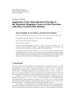
y(t)
η(t)MF
ChannelTx Rx
u
∗
(−t)
z(t) z[n]
t
= nT

s
Figure 1: An equivalent baseband model of the radio channel with
receiver matched filter (MF) front-end.
The evidence integral (5) plays a crucial role in the develop-
ment of Schwarz’s approach to model order estimation [10]
(Bayesian information criterion), as well as in a Bayesian in-
terpretation of Rissanen’s MDL principle and its variations
[5, 11, 12]. Maximizing (5) with respect to the unknown
model H
i
is known as the evidence maximization procedure,
or evidence procedure (EP) [13, 14].
Equations (3), (4), and (5) form the theoretical frame-
work for our joint model and parameter estimation. The esti-
mation algorithm is based on relevance vector machines. Rel-
evance vector machines (RVM), originally proposed by Tip-
ping [15], are an example of the marginal estimation method
that, for a set of hypotheses H
i
, iteratively approximates (1)
by alternating between the model selection, that is, maxi-
mizing (5)withrespecttoH
i
, and inferring the correspond-
ing model parameters from maximization of (3). RVMs have
been initially proposed to find sparse solutions to general lin-
ear problems. However, they can be quite effectively adapted
to the estimation of the impulse response of wireless chan-
nels, thus resulting in an effec tive channel parameter estima-
tion and model selection scheme within the Bayesian frame-

work.
The material presented in the paper is organized as fol-
lows: Section 2 introduces the signal model of the wire-
less channel and the used notation; Section 3 explains the
framework of the EP in the context of wireless channels. In
Section 4 we explain how model selection is implemented
within the presented framework and discuss the relation-
ship between the EP and the MDL criterion for model se-
lection. Finally, Section 5 presents some application results
illustrating the performance of the RVM-based estimator in
syntheticaswellasinactualwirelessenvironments.
2. CHANNEL ESTIMATION USING
PULSE-COMPRESSION TECHNIQUE
Channel estimation usually consists of two steps: (1) send-
ing a specific sounding sequence s(t) through the channel
and observing the response y(t) at the other end, and (2) es-
timating the channel parameters from the matched-filtered
received signal z(t)(Figure 1). It is common to represent
the multipath channel response as the sum of delayed and
weighted Dirac impulses, with each impulse representing one
individual multipath component (see, e.g., [16, Section 5]).
Such special structure of the channel impulse response im-
plies that the filtered signal z(t) should have a sparse struc-
ture. Unfortunately, this sparse structure is often obscured
by additive noise and temporal dispersion due to the finite
bandwidth of the transmitter and receiver hardwares. This
Dmitriy Shutin et al. 3
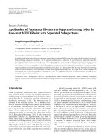
s(t)
t
···

T
p
T
u
= MT
p
T
f
Figure 2: Sounding sequence s(t).
motivates the application of algorithms capable of recover-
ing this sparse structure from the measurement data.
Let us consider an equivalent baseband channel sound-
ing scheme shown in Figure 1. The sounding signal s(t)
(Figure 2) consists of periodically repeated burst waveforms
u(t), that is, s(t)
=

∞
i=−∞
u(t−iT
f
), where u(t)hasduration
T
u
≤ T
f
andisformedasu(t) =

M−1
m=0

b
m
p(t − mT
p
). The
sequence b
0
···b
M−1
is the known sounding sequence con-
sisting of M chips, and p(t) is the shaping pulse of duration
T
p
, MT
p
= T
u
. Furthermore, we assume that the receiver
(Rx) is equipped with a planar antenna array consisting of P
sensors located at positions s
1
, , s
P
∈ R
2
with respect to an
arbitrary reference point. Let us now assume that the maxi-
mum absolute Doppler frequency of the impinging waves is
much smaller than the inverse of a single burst duration 1/T
u

.
This low Doppler frequency assumption is equivalent to as-
suming that, within a single observation window equivalent
to the period of the sounding sequence, we can safely neglect
the influence of the Doppler shifts.
The received signal vector y(t)
∈ C
P×1
for a single burst
waveform is given as [2]
y(t)
=
L

l=1
a
l
c

φ
l

e
j2πν
l
t
u

t − τ
l


+ η(t). (6)
Here, a
l
, τ
l
,andν
l
are respectively the complex gain,
the delay, and the Doppler shift of the lth multipath
component. The P-dimensional complex vector c(φ
l
) =
[c
1
(φ
l
), , c
P
(φ
l
)]
T
is the steering vector of the ar-
ray. Provided the coupling between the elements can
be neglected, its components are given as c
p
(φ
l
) =

f
p
(φ
l
)exp(j2πλ
−1
e(φ
l
), s
p
)withλ, e(φ
l
)and f
p
(φ
l
)denot-
ing the wavelength, the unit vector in
R
2
pointing in the
direction of the incoming wavefront determined by the az-
imuth φ
l
, and the complex elec tric field pattern of the pth
sensor, respectively. The additive term η(t)
∈ C
P×1
is a
vector-valued complex white Gaussian noise process, that is,

the components of η(t) are independent complex Gaussian
processes with double-sided spectral density N
0
.
The receiver front-end consists of a matched filter (MF)
matched to the tr ansmitted sequence u(t). Under the low
Doppler frequency assumption the term e
j2πν
l
t
stays time-
invariant within a single burst duration, that is, equal to a
complex constant that can be incorporated in the complex
gain a
l
. The signal z(t) at the output of the MF is then given
as
z(t)
=
L

l=1
a
l
c

φ
l

R

uu

t − τ
l

+ ξ(t), (7)
where R
uu
(t) =

u(t

)u
∗
(t + t

)dt

is the autocorrelation
function of the burst waveform u(t)andξ( t)
=

η(t

)u
∗
(t +
t

)dt


is a spatially white P-dimensional vector with each ele-
ment being a zero-mean wide-sense stationary (WSS) Gaus-
sian noise with autocorrelation function
R
ξξ
(t) = E

ξ
p
(t

)ξ
∗
p
(t + t

)

=
N
0
R
uu
(t),
E

ξ
p
(t


)ξ
p
(t + t

)

=
0.
(8)
Here E
{·} denotes the expectation operator. Equation (7)
states that the MF output is a linear combination of L scaled
and delayed kernel functions R
uu
(t−τ
l
), weighted across sen-
sors as given by the components of c(φ
l
) and observed in the
presence of the colored noise ξ(t).
In practice, however, the output of the MF is sampled
with the sampling period T
s
≤ T
p
, resulting in PN-tuples of
the MF output, where N is the number of MF output sam-
ples. By collecting the output of each sensor into a vector, we

can rewrite (7)inavectorform:
z
p
= Kw
p
+ ξ
p
, p = 1 ···P,(9)
wherewehavedefined
z
p
=

z
p
[0], z
p
[1], , z
p
[N −1]

T
,
w
p
=

a
1
c

p

φ
1

, , a
L
c
p

φ
L

T
,
ξ
p
=

ξ
p
[0], ξ
p
[1], , ξ
p
[N −1]

T
.
(10)

The additive noise vectors ξ
p
, p = 1 ···P, possess the
following properties that will be exploited later:
E

ξ
p

= 0, E

ξ
m
ξ
H
k

= 0,form/= k, (11)
E

ξ
p
ξ
H
p

=
Σ = N
0
Λ,whereΛ

i, j
= R
uu

(i − j)T
s

.
(12)
Note that (12) follows directly from (8). The matrix K,
also called the design mat rix, accumulates the shifted and
sampled versions of the kernel function R
uu
(t). It is con-
structed as K
= [r
1
, , r
L
], with r
l
= [R
uu
(−τ
l
), R
uu
(T
s
−

τ
l
), , R
uu
((N −1)T
s
− τ
l
)]
T
.
In general, the channel estimation problem is posed as
follows: given the measured sampled signals z
p
, p = 1···P,
determine the order L of the model and estimate optimally
(with respect to some quality criterion) al l multipath param-
eters a
l
, τ
l
,andφ
l
,forl = 1 ···L. In this contribution, we re-
strict ourselves to the estimation of the model order L along
with the vector w
p
, rather than of the constituting parame-
ters τ
l

, φ
l
,anda
l
. We will also quantize, although arbitrarily
fine,
2
the search space for the multipath delays τ
l
.Thus,we
2
There is actually a limit beyond which it makes no sense to make the
search grid finer, since it will not decrease the variance of the estimates,
which is lower-bounded by the Crammer-Rao bound [2].
4 EURASIP Journal on Advances in Signal Processing
do not try to estimate the path delays with infinite resolu-
tion, but rather fix the delay values to be located on a grid
with a given mesh determining the quantization error. The
size of the delay search space L
0
and the resulting quantized
delays T
={T
1
, , T
L
0
} form the initial model hypothesis
H
0

, which would manifest itself in the L
0
columns of the de-
sign matrix K. This allows to formulate the channel estima-
tion problem as a standard linear problem to which the RVM
algorithm can be applied.
As it can be seen, our idea lies in finding the closest
approximation of the continuous-time model (7) with the
discrete-time equivalent (9). By incorporating the model se-
lection in the analysis, we also strive to find the most com-
pact representation (in terms of the number of components),
while preserving good approximation quality. Thus, our goal
is to estimate the channel parameters w
p
as well as to deter-
mine how many multipath components L
≤ L
0
are present in
the measured impulse response. The application of the RVM
framework to solve this problem follows in the next section.
3. EVIDENCE MAXIMIZATION, RELEVANCE VECTOR
MACHINES, AND WIRELESS CHANNELS
We begin our analysis following the steps outlined in
Section 1. In order to ease the algorithm description we first
assume that P
= 1, that is, only a single sensor is used. Ex-
tensions to the case P>1 are carried out later in Section 3.2.
To simplify the notations we also drop the subscript index p
in our further notations.

From (9) it follows that the observation vector z is a lin-
ear combination of the vectors from the column-space of K,
weighted according to the parameters w andembeddedin
the correlated noise ξ. In order to correctly assess the order
of the model, it is imperative to take the noise process into
account. It follows from (12) that the covariance matrix of
the noise is proportional to the unknown spectral height N
0
,
which should therefore be estimated from the data. Thus,
the model hypotheses H
i
should include the term N
0
.In
the following analysis we assume that β
= N
−1
0
is Gamma-
distributed [15], with the corresponding probability density
function (pdf) given as
p(β
| κ, υ) =
κ
υ
Γ(υ)
β
υ−1
exp(−κβ), (13)

with parameters κ and υ predefined so that (13)accurately
reflects our a priori information about N
0
. In the absence of
any a priori knowledge one can make use of a noninforma-
tive (i.e., flat in the logarithmic domain) prior by fixing the
parameters to small values κ
= υ = 10
−4
[15]. Furthermore,
to steer the model selection mechanism, we introduce an ex-
tra parameter (hyperparameter) α
l
, l = 1 ···L
0
,foreach
column in K. This parameter measures the contr ibution or
relevance of the corresponding weight w
l
in explaining the
data z from the likelihood p(z
| w
i
, H
i
). This is achieved by
specifying the prior p(w
| α) for the model weights:
p(w
| α) =

L
0

l=1
α
l
π
exp

−


w
l


2
α
l

. (14)
High values of α
l
will render the contribution of the cor-
responding column in the matrix K “irrelevant,” since the
weight w
l
is likely to have a very small value (hence they
are termed relevance hyperparameters). This will enable us
to prune the model by setting the corresponding weight w

l
to zero, thus effectively removing the corresponding column
from the matrix and the corresponding delay T
l
from the de-
lay search space T . We also see that α
−1
l
is nothing else as
the prior variance of the model weight w
l
. Also note that the
prior (14) implicitly assumes statistical independence of the
multipath contributions.
To complete the Bayesian framework, we also specify the
prior over the hyperparameters. Similarly to the noise con-
tribution, we assume the hyperparameters α
l
to be Gamma-
distributed with the corresponding pdf
p(α
| ζ,) =
L

l=1
ζ

Γ()
α


−
1
l
exp

−
ζα
l

, (15)
where ζ and
 arefixedatsomevaluesthatensureanap-
propriate form of the prior. Again, we can make this prior
noninformative by fixing ζ and
 to small values, for exam-
ple,
 = ζ = 10
−4
.
Now, let us define the hypothesis H
i
more formally. Let
P (S) be a power set consisting of all possible subsets of basis
vector indices S
={1 ···L
0
},andi→P (i) the indexing of
P (S) such that P (0)
= S. Then for each index value i the
hypothesis H

i
is the set H
i
={β; α
j
, j ∈ P (i)}. Clearly, the
initial hypothesis H
0
={β; α
j
, j ∈ S} includes all possible
potential basis functions.
Now we are ready to outline the learning algorithm that
estimates the model parameters w, β, and hyperparameters α
from the measurement data z.
3.1. Learning algorithm
Basically, learning consists of inferring the values of w
i
and
the hypothesis H
i
that maximize the posterior (2): p(w
i
, H
i
|
Z) ≡ p(w
i
, α
i

, β | z). Here α
i
denotes the vector of all ev-
idence hyperparameters associated with the ith hypothesis.
The latter expression can also be rewritten as
p(w, α, β
| z) = p(w | z, α, β)p(α, β | z). (16)
The explicit dependence on the hypothesis index i has been
dropped to simplify the notation. We recognize that the first
term p(w
| z, α, β)in(16) is the weight posterior and the
other one p(α, β
| z) is the hypothesis posterior. From this
point we can start with the Bayesian two-step analysis as has
been indicated before.
Assuming the parameters α and β are known, estimation
of model parameters consists of finding values w that max-
imize p(w
| z, α, β). Using Bayes’ rule we can rewrite this
posterior as
p(w
| z, α, β) ∝ p(z | w, α, β)p(w | α, β). (17)
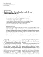
Consider the Bayesian graphical model [17]inFigure 3.
This graph captures the relationship between different vari-
ables involved in (16). It is a useful tool to represent the de-
pendencies among the variables involved in the analysis in
Dmitriy Shutin et al. 5
α
1
α

2
α
L
w
1
w
2
w
L
z[0]
z[N
− 1]
β
···
···
···
Figure 3: Graph representing the discrete-time model of the wire-
less channel.
order to factor the joint density function into contributing
marginals.
It immediately follows from the structure of the graph in
Figure 3 that p(z
| w, α, β) = p(z | w, β)andp(w | α, β) =
p(w | α), that is, z and α are conditionally independent given
w and β,andw and β are conditionally independent given α.
Thus, (17)isequivalentto
p(w
| z, α, β) ∝ p(z | w, β)p(w | α), (18)
where the second factor on the right-hand side is given in
(14). The first term is the likelihood of w and β given the

data. From (9) it follows that
p(z
| w, β) =
exp

− (z − Kw )
H
βΛ
−1
(z − Kw )

π
N


β
−1
Λ


. (19)
Since both right-hand factors in (18) are Gaussian densities,
p(w
| z, α, β) is also a Gaussian density with the covariance
matrix Φ and mean μ given as
Φ
=

A + βK
H

Λ
−1
K

−1
, (20)
μ
= βΦK
H
Λ
−1
z. (21)
The matrix A
= diag(α) is a diagonal matrix that contains
the evidence parameters α
l
on its main diagonal. Clearly, μ
is a maximum a-posteriori (MAP) estimate of the parame-
ter vector w under the hypothesis H
i
,withΦ being the co-
variance matrix of the resulting estimates. This completes the
model fitting step.
Ournextstepistofindparametersα and β that maxi-
mize the hypothesis posterior p(α, β
| z)in(16). This den-
sity function can be represented as p(α, β
| z) ∝ p(z |
α, β)p(α, β), where p(z | α, β) is the evidence term and
p(α, β)

= p(α)p(β) is the hypothesis prior. As it was men-
tioned earlier, it is quite reasonable to choose noninformative
priors since we would like to give all possible hypotheses H
i
an equal chance of being valid. This can be achieved by set-
ting ζ,
, κ,andυ to very small values. In fact, it can be easily
concluded (see derivations in the appendix) that maximum
of the evidence p(z
| α, β) coincides with the maximum of
p(z
| α, β)p(α, β) when ζ =  = κ = υ = 0, which effectively
results in the noninformative hyperpriors for α and β.
This formulation of prior distributions is related to au-
tomatic relevance determination (ARD) [14, 18]. As a con-
sequence of this assumption, the maximization of the model
posterior is equivalent to the maximization of the evidence,
which is known as the evidence procedure [13].
Theevidencetermp(z
| α, β) c an be expressed as
p(z
| α, β) =

p(z | w, β)p(w | α)dw
=
exp

−
z
H


β
−1
Λ + KA
−1
K
H

−1
z

π
N


β
−1
Λ + KA
−1
K
H


,
(22)
which is equivalent to (5), where conditional independencies
between variables have been used to simplify the integrands.
In the Bayesian literature this quantity is known as marginal
likelihood and its maximization with respect to the unknow n
hyperparameters α and β is a type-II maximum likelihood

method [19]. To ease the optimization, several terms in (22)
can be expressed as a function of the weight posterior param-
eters μ and Φ as given by (20)and(21). Then, by taking the
derivatives of the logarithm of (22)withrespecttoα and β
and by setting them to zero, we obtain its maximizing values
as (see also the appendix)
α
l
=
1
Φ
ll
+


μ
l


2
, (23)
β
−1
=
tr

ΦK
H
Λ
−1

K

+(z − Kμ)
H
Λ
−1
(z − Kμ)
N
. (24)
In (23) μ
l
and Φ
ll
denote the lth element of, respectively, the
vector μ, and the main diagonal of the matrix Φ. Unlike the
maximizing values obtained in the original RVM paper [15,
equation (18)], (24) is derived for the extended, more gen-
eral case of colored additive noise ξ with the corresponding
covariance matrix β
−1
Λ ar ising due to the MF processing at
the receiver. Clearly, if the noise is assumed to be white, ex-
pressions (23)and(24) coincide with those derived in [15].
Also note that α and β are dependent as it can be seen from
(23)and(24).
Thus, for a particular hypothesis H
i
the learning algo-
rithm proceeds by repeated application of (20)and(21), al-
ternated with the update of the corresponding evidence pa-

rameters α
i
and β from (23)and(24), as depic ted in Figure 4,
until some suitable convergence criterion has been satisfied.
Provided a good initialization of α
[0]
i
and β
[0]
is chosen,
3
the
scheme in Figure 4 converges after j iterations to the station-
ary point of the system of coupled equations (20), (21), (23),
and (24). Then, the maximization (1) is performed by select-
ing the hypothesis that results in the highest posterior (2).
In practice, however, we will observe that during the rees-
timation some of the hyperparameters α
l
diverge, or, in fact,
become numerically indistinguishable from infinity given the
computer accuracy.
4
Thedivergenceofsomeofthehyper-
parameters enables us to approximate (1) by performing an
3
Later in Section 5 we consider several rules for initializing the hyperpa-
rameters.
4
In the finite sample size case, however, this will only happen in the

high SNR regime. Otherwise, α
l
will take large but still finite values. In
Section 4.1 we elaborate more on the conditions that lead to conver-
gence/divergence of this learning scheme.
6 EURASIP Journal on Advances in Signal Processing
Hypothesis H
i
Parameter
posteriors
Eq. (20), (21)
Hypothesis
update
Eq. (23), (24)
α
[0]
i
, β
[0]
Φ
[ j]
i
, μ
[ j]
i
α
[ j]
i
, β
[ j]

Figure 4: Iterative learning of the parameters; the superscript [j]
denotes the iteration index.
on-line model selection: starting from the initial hypothesis
H
0
, we prune the hyperparameters that become larger than
a certain threshold as the iterations proceed by setting them
to infinity. In turn, this sets the corresponding coefficient w
l
to zero, thus “switching off ” the lth column in the kernel
matrix K and removing the delay T
l
from the search space
T .Thiseffectively implements the model selection by cre-
ating smaller hypotheses H
i
< H
0
(withfewerbasisfunc-
tions) without performing an exhaustive search over all the
possibilities. The choice of the threshold will be discussed in
Section 4.
3.2. Extensions to multiple channel observations
In this subsection we extend the above analysis to multiple
channel observations or multiple antenna systems. When de-
tecting multipath components any additional channel mea-
surement (either in time, by observing several periods of the
sounding sequence u(t), or in space, by using multiple sen-
sor antenna) can be used to increase detection quality. Of
course, it is important to make sure that the multipath com-

ponents are time-invariant within the observation interval.
The basic idea how to incorporate several channel observa-
tions is quite simple: in the original formulation each hyper-
parameter α
l
was used to control a single weight w
l
and thus
the single component. Having several channel observations,
a single hyperparameter α
l
now controls weights represent-
ing contribution of the same physical multipath component,
but present in the different channel observations.
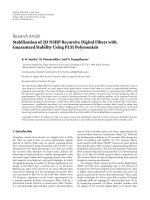
Usage of a single parameter in this case expresses the
channel coherence property in the Bayesian framework. The
corresponding graphical model that illustrates this idea for a
single hyperparameter α
l
is depicted in Figure 5. It is inter-
esting to note that similar ideas, though in a totally different
context, were adapted to train neural networks by allowing
a single hyperparameter to control a group of weights [18].
Note that it is also possible to introduce an individual hyper-
parameter α
p,l
for each weight w
p,l
, but this eventually decou-
ples the problem into P separate one-dimensional problems

and, as the result, any dependency between the consecutive
channels is ignored.
Now,letusreturnto(9). It can be seen that the weights
w
p
capture the structure induced by multiple antennas.
However, for the moment we ignore this structure and treat
the components of w
p
as a wide-sense stationary (WSS)
α
l
w
2,l
w
1,l
z
1
[n]
z
2
[n]
β
w
P,l
z
P
[n]
Figure 5: Usage of α
l

in a multiple-observation discrete-time wire-
less channel model to represent P coherent channel measurements.
process over the individual channels, p = 1 ···P.Wewill
also allow each sensor to have a different MF. This might
not necessarily be the case for wireless channel sounding,
but thus a more general situation can be considered. Differ-
ent matched filters result in different design matrices K
p
,and
thus different noise covariance matrices Σ
p
, p = 1 ···P.We
will however require that the variance of the input noise re-
mains the same and equals N
0
= β
−1
for all channels, so that
Σ
p
= N
0
Λ
p
, and the noise components are statistically inde-
pendent among the channels. Then, by defining

Σ = β
−1
⎡

⎢
⎢
⎣
Λ
1
0
.
.
.
0 Λ
P
⎤
⎥
⎥
⎦
,

A =
⎡
⎢
⎢
⎣
A0
.
.
.
0A
⎤
⎥
⎥

⎦

 
P×P block matrix
,

K =
⎡
⎢
⎢
⎣
K
1
0
.
.
.
0K
P
⎤
⎥
⎥
⎦
, z =
⎡
⎢
⎢
⎣
z
1

.
.
.
z
P
⎤
⎥
⎥
⎦
, w =
⎡
⎢
⎢
⎣
w
1
.
.
.
w
P
⎤
⎥
⎥
⎦
,
(25)
we rewrite (9)as
z =


K w +

ξ. (26)
A crucial point of this system representation is that the hy-
perparameters α
l
are shared by P channels as it can be seen
in the structure of the matrix

A. This will have a correspond-
ing effect on the hyperparameter reestimation algorithm.
From the structural equivalence of (9)and(26)wecan
easily infer that (20)and(21) are modified as follows:
Φ
p
=

A + βK
H
p
Λ
−1
p
K
p

−1
, (27)
μ
p

= βΦ
p
K
H
p
Λ
−1
p
z
p
, p = 1 ···P. (28)
Dmitriy Shutin et al. 7
The expressions for the hyperparameter updates become
a bit more complicated but are still straight-forward to com-
pute. It is shown in the app endix that
α
l
=
P

P
p=1

Φ
p,ll
+


μ
p,l



2

, (29)
N
0
= β
−1
=
1
NP

P

p=1
tr

Φ
p
K
H
p
Λ
−1
p
K
p

+

P

p=1

z
p
− K
p
μ
p

H
Λ
−1
p

z
p
− K
p
μ
p


,
(30)
where μ
p,l
is the lth element of the MAP estimate of the pa-
rameter vector w

p
given by (28), and Φ
p,ll
is the lth element
on the main diagonal of Φ
p
from (27). Comparing the latter
expressions with those developed for the single channel case,
we observe that (29)and(30) use multiple channels to im-
prove the estimates of the noise spectral height and channel
weight hyperparameters. They also offer more insight into
the physical meaning of the hyperparameters α. On the one
hand, the hyperparameters are used to regularize the matr ix
inversion (27), needed to obtain the MAP estimates of the
parameters w
p,l
and their corresponding variances. On the
other hand, they act as the inverse of the second noncentral
moments of the coefficients w
p,l
, as can be seen from (29).
4. MODEL SELECTION AND BASIS PRUNING
The ability to selec t the best model to represent the mea-
sured data is an important feature of the proposed scheme,
and thus it is paramount to consider in more detail how the
model selection is effectively achieved. In Section 3.1 we ha ve
briefly mentioned that during the learning phase many of
the hyperparameters α
l
’s tend to large values, meaning that

the corresponding weights w
l
’s will cluster around zero ac-
cording to the prior (14). This will allow us to set these co-
efficients to zero, thus effectively pruning the corresponding
basis function from the design matrix. However the question
how large a hyperparameter has to grow in order to prune
its corresponding basis function has not yet been discussed.
In the original RVM paper [15], the author suggests using
a threshold α
th
to prune the model. The empirical evidence
collected by the author suggests setting the threshold to “a
sufficiently large number” (e.g., α
th
= 10
12
). However, our
theoretical analysis presented in the following section will
show that such high thresholds are only meaningful in very
high SNR regimes, or if the number of channel observations
P is sufficiently large. In more general, and often more realis-
tic, scenarios such high thresholds are absolutely impractical.
Thus, there is a need to study the model selection problem in
the context of the presented approach more rigorously.
Below, we present two methods for implementing model
selection within the proposed algorithm. The first method
relies on the statistical properties of the hyperparameters α
l
,

when the update equations (27), (28), (29), and (30)con-
verge to a stationary point. The second method exploits the
relationship that we will establish between the proposed
scheme and the minimum description length principle [4, 8,
20, 21], thus linking the EP to this classical model selection
approach.
4.1. Statistical analysis of the hyperparameters
in the stationary point
The decision to keep or to prune a basis function from the de-
sign matrix is based purely on the value of the corresponding
hyperparameter α
l
. In the following we analyze the conver-
gence properties of the iterative learning scheme depicted in
Figure 4 using expressions (27), (28), (29), and (30), and the
resulting distribution of the hyperparameters once conver-
gence is achieved.
We start our analysis of the evidence parameters α
l
by making some simplifications to make the derivations
tractable.
(i) P channels are assumed.
(ii) The same MF is used to process each of the P sensor
output signals, that is, K
p
= K and Σ
p
= Σ = β
−1
Λ,

p
= 1 ···P.
(iii) The noise covariance matrix Σ is known, and B
= Σ
−1
.
(iv) We assume the presence of a single multipath compo-
nent, that is, L
= 1, with known delay τ. Thus, the
design matrix is given as K
= [r(τ)], where r(τ) =
[R
uu
(−τ), R
uu
(T
s
−τ), , R
uu
((N − 1)T
s
−τ)]
T
is the
associated basis function.
(v) The hyperparameter associated with this component
is denoted as α.
Our goal is to consider the steady-state solution α
∞
for

hyperparameter α in this simplified scenario. In this case (27)
and (28) simplify to
φ
=

α + r(τ)
H
Br(τ)

−1
,
μ
p
= φK
H
Bz
p
=
r(τ)
H
Bz
p
α + r(τ)
H
Br(τ)
, p
= 1 ···P.
(31)
Inserting these two expressions into (29) y ields
α

−1
=
1
α + r(τ)
H
Br(τ)
+

p


r(τ)
H
Bz
p
/

α + r(τ)
H
Br(τ)



2
P
.
(32)
From (32) the solution α
∞
is easily found to be

α
∞
=

r(τ)
H
Br(τ)

2
(1/P)

p


r(τ)
H
Bz
p


2
− r(τ)
H
Br(τ)
. (33)
A closer look at (33) reveals that the right-hand side ex-
pression might not always be positive since the denominator
canbenegativeforsomevaluesofz
p
. This contradicts the

assumption that the hyperparameter α is positive.
5
A further
5
Recall that α
−1
is the prior variance of the corresponding parameter w.
This constrains α to be nonnegative.
8 EURASIP Journal on Advances in Signal Processing
analysis of (32) reveals that (29)convergesto(33)ifandonly
if the denominator of (33)ispositive:
1
P

p


r(τ)
H
Bz
p


2
> r(τ)
H
Br(τ). (34)
Otherwise, the iterative learning scheme depicted in Figure 4
diverges, that is, α
∞

=∞. This can be inferred by interpreting
(29) as a nonlinear dynamic system that, at iteration j,maps
α
[ j−1]
into the updated value α
[ j]
. The nonlinear mapping is
given by the right-hand side of (29), where the quantities Φ
p
and μ
p
depend on the values of the hyperparameters at it-
eration j
− 1. In Figure 6 we show several iterations of this
mapping that illustrate how the solution trajectories evolve.
If condition (34) is satisfied, the sequence of solutions
{α
[ j]
}
converges to a stationary point (Figure 6(a))givenby(33).
Otherwise,
{α
[ j]
} diverges (Figure 6(b)). Thus, (32) is a sta-
tionary point only provided the condition (34) is satisfied:
α
∞
=
⎧
⎪

⎪
⎨
⎪
⎪
⎩

r(τ)
H
Br(τ)

2

p


r(τ)
H
Bz
p


2
/P−r(τ)
H
Br(τ)
; cond. (34 ) is satisfied,
∞; otherwise.
(35)
Practically, this means that for a given measurement z
p

,and
known noise matrix B, we can immediately decide whether a
given basis function r(τ) should be included in the basis by
simply checking if (34)issatisfiedornot.
A similar analysis is performed in [22], where the behav-
ior of the likelihood function with respect to a single parame-
ter is studied. The obtained convergence results coincide with
ours when P
= 1. Expression (34) is, however, more gen-
eral and accounts for multiple channel observations and col-
ored noise. In [22] the authors also suggest that testing (34)
for a given basis function r(τ)issufficient to find a sparse
representation and no further pruning is necessary. In other
words, each basis function in the design matrix K is subject
to the test (34) and, if the test fails, that is, (34) does not hold
for the basis function under test, the basis function is pruned.
In case of wireless channels, however, we have exper-
imentally observed that even in simulated high-SNR sce-
narios such pruning results in a significantly overestimated
number of multipath components. Moreover, it can be in-
ferred from (34) that, as the SNR increases, the number of
functions pruned with this approach decreases, resulting in
less and less sparse representations. This motivates us to per-
form a more detailed analysis of (35).
Let us slightly modify the assumptions we made earlier.
We now assume that the multipath delay τ is unknown. The
design matrix is constructed similarly but this time K
= [r
l
],

where
r
l
=

R
uu

−
T
l

, , R
uu

(N −1)T
s
− T
l

T
(36)
is the basis function associated with the delay T
l
∈ T used in
our discrete-time model. Under these assumptions the input
signal z
p
is nothing else but the basis function r(τ) scaled
1.03

1.04
1.05
1.06
1.07
1.08
1.09
1.1
1.11
1.12
α
[ j]
11.05 1.11.15
α
[ j−1]
Nonlinear mapping
α
[ j]
= α
[ j−1]
Iteration trajectory 1
Iteration trajectory 2
(a)
0
10
20
30
40
50
60
70

80
α
[ j]
010203040506070
α
[ j−1]
Nonlinear mapping
α
[ j]
= α
[ j−1]
Iteration trajectory 1
Iteration trajectory 2
(b)
Figure 6: Evolution of the two representative solution trajectories
for two cases: (a)
{α
[ j]
} converges, (b) {α
[ j]
} diverges.
and embedded in the additive complex zero-mean Gaussian
noise with covariance matrix Σ, that is,
z
p
= w
p
r(τ)+ξ
p
. (37)

Let us further assume that w
p
∈ C, p = 1 ···P,areun-
known but fixed complex scaling factors. In further deriva-
tions we assume, unless explicitly stated otherwise, that the
condition (34) is satisfied for the basis r
l
. By plugging (37)
Dmitriy Shutin et al. 9
into (33) and rearranging the result with respect to α
−1
∞
we
arrive at
α
−1
∞
=


r
H
l
Br(τ)


2

p



w
p


2
P


r
H
l
Br
l


2
+
2

p
Re

w
p
r
H
l
Br(τ)ξ
H

p
Br
l

P


r
H
l
Br
l


2
+
r
H
l
B


p
ξ
p
ξ
H
p

Br

l
P


r
H
l
Br
l


2
−
1
r
H
l
Br
l
.
(38)
Now, we consider two scenarios. In the first scenario τ
=
T
l
∈ T , that is, the discrete-time model matches the ob-
served signal. Although unrealistic, this allows to study the
properties of α
−1
∞

more closely. In the second scenario, we
study what happens if the discrete-time model does not
match perfectly the measured signal. This case helps us to
define how the model selection rules have to be adjusted to
consider possible misalignment of the path component de-
lays in the model.
4.1.1. Model match: τ
= T
l
In this situation, r
l
= r(τ), and thus (38) can be further sim-
plified according to
α
−1
∞
=

p


w
p


2
P
+
2


p
Re

w
p
ξ
p
Br
l

P

r
H
l
Br
l

+
r
H
l
B


p
ξ
p
ξ
H

p

Br
l
P

r
H
l
Br
l

2
−
1
r
H
l
Br
l
,
(39)
where the only random quantity is the additive noise term ξ
p
.
This allows us to study the statistical properties of the finite
stationary point in (35).
Equation (39) shows how the noise and multipath com-
ponent contribute to α
−1

∞
.Ifallw
p
are set to be zero, that is,
there is no multipath component, then α
−1
∞
= α
−1
n
reflects
only the noise contribution:
α
−1
n
=
r
H
l
B


p
ξ
p
ξ
H
p

Br

l
P

r
H
l
Br
l

2
−
1
r
H
l
Br
l
. (40)
On the other hand, in the absence of noise, that is, in the
infinite SNR case, the corresponding hyperparameter α
−1
∞
in-
cludes the contribution of the multipath component
6
α
−1
s
:
α

−1
s
=

p


w
p


2
P
+
2

p
Re

w
p
ξ
H
p
Br
l

P

r

H
l
Br
l

. (41)
In a realistic case, both noise and multipath component are
present, and α
−1
∞
consists of the sum of two contributions
6
Actually, the second term in the resulting expression vanishes in a per-
fectly noise-free case, and then α
−1
s
=

p
|w
p
|
2
/P.
α
−1
∞
= α
−1
s

+ α
−1
n
. Both quantities α
−1
s
and α
−1
n
are random
variables with pdf’s depending on the number of channel ob-
servations P, the basis function r
l
, and the noise covariance
matrix Σ. In the sequel we analyze their statistical properties.
We first consider α
−1
s
. The first term on the right-hand
side of (41) is a deterministic quantity that equals the average
power of the multipath component. The second one, on the
other hand, is random. The product Re
{w
p
ξ
H
p
Br
l
} in (41)

is recognized as the cross-correlation between the additive
noise term and the basis function r
l
. It is Gaussian distributed
with expectation and variance given as
E

2

p
Re

w
p
ξ
H
p
Br
l

P

r
H
l
Br
l


=

0,
E

2

p
Re

w
p
ξ
H
p
Br
l

P

r
H
l
Br
l


2

=
2


p


w
p


2
P
2

r
H
l
Br
l

,
(42)
respectively, where E
{·} denotes the expectation operator.
Thus, α
−1
s
is distributed as
α
−1
s
∼ N



p


w
p


2
P
,
2

p


w
p


2
P
2

r
H
l
Br
l



, (43)
which is a normal distribution with the mean given by the av-
erage power of the multipath component and variance pro-
portional to this power.
Now, let us consider the term α
−1
n
.In(40) the only ran-
dom element is

P
p
=1
ξ
p
ξ
H
p
. This random matrix is known to
have a complex Wishart distribution [23, 24] with the scale
matrix Σ and P degrees of freedom. Let us denote
c
=
Br
l
√
Pr
H
l

Br
l
, x = c
H
P

p=1
ξ
p
ξ
H
p
c. (44)
It can be shown that x is Gamma-distributed, that is, x ∼
G(P, σ
2
c
), with the shape parameter P and the scale parameter
σ
2
c
given as
σ
2
c
= c
H
Σc =
1
P


r
H
l
Br
l

. (45)
The pdf of x reads
p

x | P, σ
2
c

=
x
P−1
Γ(P)

σ
2
c

P
e
−x/σ
2
c
. (46)

The mean and the variance of x are easily computed to be
E
{x}=Pσ
2
c
=
1
r
H
l
Br
l
,
Var
{x}=P

σ
2
c

2
=
1
P

r
H
l
Br
l


2
.
(47)
Taking the term
−1/(r
H
l
Br
l
)in(40) into account, we intro-
duce a variable
α
−1
n
: a zero mean random variable with the
pdf
p
α
−1
n

x | P, σ
2
c

=

x − E{x}


P−1
Γ(P)

σ
2
c

P
e
−(x−E{x})/σ
2
c
, (48)
10 EURASIP Journal on Advances in Signal Processing
whichisequivalentto(46), but shifted so as to correspond
to a zero-mean distribution. However, it is known that only
positive values of α
−1
n
occur in practice. The probability mass
of the negative part of (48) equals the probability that the
condition (34) is not satisfied and the resulting α
∞
eventually
diverges to infinity and is pruned. Taking this into account
the pdf of α
−1
n
reads
p

α
−1
n
(x) = P
n
δ(x)+

1 − P
n

I
+
(x)

p
α
−1
n

x | P, σ
2
c

,
(49)
where δ(
·) denotes a Dirac delta function, P
n
is defined as
P

n
=

0
−1/(r
H
l
Br
l
)

p
α
−1
n

x | P, σ
2
c

dx, (50)
and I
+
(·) is the indicator function of the set of positive real
numbers:
I
+
(x) =
⎧
⎨

⎩
0 x ≤ 0,
1 x>0.
(51)
A closer look at (49) shows that as P increases the variance of
the Gamma distribution decreases, with α
−1
n
concentrating
at zero. In the limiting case as P
→∞,(49)convergestoa
Dirac delta function localized at zero, that is, α
n
=∞. This
allows natural pruning of the corresponding basis function.
This situation is equivalent to averaging out the noise, as the
number of channel observations grows. Practically, however,
P stays always finite, which means that (43)and(49)havea
certain finite variance.
The pruning problem can now be approached from the
perspective of classical detection theory. To prune a basis
function, we have to decide if the corresponding value of
α
−1
has been generated by the noise distribution (49), that
is, the null hypothesis, or by the pdf of α
−1
s
+ α
−1

n
, that is, the
alternative hypothesis. Computing the latter is difficult. The
problem might be somewhat relaxed by taking the assump-
tion that α
−1
s
and α
−1
n
are statistically independent. However
proving the plausibility of this assumption is difficult. Even
if we were successful in finding the analytical expression for
the pdf of the alternative hypothesis, such model selection
approach is hampered by our inability to evaluate (43) since
the gains w
p
’s are not known a priori. However, we can still
use (49) to select a threshold.
Recall that the presented algorithm allows to learn (esti-
mate) the noise spectral height N
0
= β
−1
from the measure-
ments. Assuming that we know β, and, as a consequence, the
whole matrix B then, for any basis function r
l
in the design
matrix K and the corresponding hyperparameter α

l
,wecan
decide with a priori specified probability ρ that α
l
is gener-
ated by the distribution (49). Indeed, let α
−1
th
be a ρ-quantile
of (49) such that the probability P(α
−1
≤ α
−1
th
) = ρ. Since
(49) is known exactly, we can easily compute α
−1
th
and prune
all the basis functions for which α
−1
l
≤ α
−1
th
.
4.1.2. Model mismatch: τ/
= T
l
The analysis performed above relies on the knowledge

that the true multipath delay τ belongs to T . Unfortunately,
this is often unrealistic and the model mismatch τ/
∈ T
must be considered. To be able to study how the model mis-
match influences the value of the hyperparameters we have to
make a few more assumptions. Let us for simplicity select the
model delay T
l
to be a multiple of the chip period T
p
.Wewill
also need to assume a certain shape of the correlation func-
tion R
uu
(t) to make the whole analysis tractable. It may be
convenient to assume that the main lobe of R
uu
(t) can be ap-
proximated by a raised cosine function with period 2T
p
. This
approximation makes sense if the sounding pulse p(t)de-
fined in Section 2 is a square root raised cosine pulse. Clearly,
this approximation can also be applied for other shapes of the
main lobe, but the analysis of quality of such approximation
remains outside the scope of this paper.
Just as in the previous case, we can split the expression
(38) into the multipath component contribution α
−1
s

α
−1
s
=


γ(τ)


2

p


w
p


2
P
+
2

p
Re

w
p
γ(τ)ξ
H

p
Br
l

P


r
H
l
Br
l


,
(52)
where
γ(τ)
=
r
H
l
Br(τ)
r
H
l
Br
l
, (53)
and the same noise contribution α

−1
n
defined in (40). It can
be seen that the γ(τ)makes(52)differ from (41), and a s such
it is the key to the analysis of the model mismatch. Note that
this function is bounded as
|γ(τ)|≤1, with equality follow-
ing only if τ
= T
l
. Note also that in our case for |τ −T
l
| <T
p
the correlation γ(τ) is strictly positive.
Due to the properties of the sounding sequence u(t), the
magnitude of R
uu
(t)for|t| >T
p
is sufficiently small and in
our analysis of model mismatch can be safely assumed to be
zero. Furthermore, if r
l
is chosen to coincide with the mul-
tiple of the sampling period T
l
= lT
s
, then it follows from

(12) that the product r
H
l
B = r
H
l
Σ
−1
= βe
H
l
is a vector with
all elements being zero except the lth element, which is equal
to β. Thus, the product r
H
l
Br(τ)for|τ − T
l
| <T
p
must have
a form identical to that of the correlation function R
uu
(t)for
|t| <T
p
. It follows that when |τ − T
l
|≥T
p

the correlation
γ(τ) can be assumed to be zero, and it makes sense to ana-
lyze (52) only when
|τ − T
l
| <T
p
.InFigure 7 we plot the
correlation functions R
uu
(t)andγ(τ) for this case.
Since the true value of τ is unknown, we assume this pa-
rameter to be random, uniformly distributed in the interval
[T
l
−T
p
, T
l
+ T
p
]. This in turn induces corresponding distri-
butions for the random variables γ(τ)andγ(τ)
2
,whichenter,
respectively, the second and first terms on the right-hand side
of (52).
It can be shown that in this case γ(τ) ∼ B(0.5, 0.5),
where B(0.5, 0.5) is a Beta distribution [25] with both distri-
bution parameters equal to 1/2. The corresponding pdf p

γ
(x)
is given in this case as
p
γ
(x) =
1
B(0.5, 0.5)
x
−1/2
(1 − x)
−1/2
, (54)
where B(
·, ·) is a Beta-function [26]withB(0.5, 0.5) = π.
Dmitriy Shutin et al. 11
−0.2
0
0.2
0.4
0.6
0.8
1
1.2
−3T
p
−2T
p
−T
p

0
T
p
2T
p
3T
p
Delay, τ
R
uu
(t)
Sampled R
uu
(t)
(a)
−0.2
0
0.2
0.4
0.6
0.8
1
1.2
γ(τ)
−T
p
0
T
p
Delay, τ

(b)
Figure 7: Evaluated correlation functions (a) R
uu
(t) and (b) γ(τ).
It is also straight-forward to compute the pdf of the term
γ(τ)
2
:
p
γ
2
(x) =
1
π
x
−3/4
(1 −
√
x)
−1/2
. (55)
The corresponding empirical and theoretical pdf’s of
γ(τ)andγ(τ)
2
are shown in Figure 8 .
Now we have to find out how this information can be uti-
lized to design an appropriate threshold. In the case of a per-
fectly matched model the threshold is selected based on the
noise distribution (49). In the case of a model mismatch, the
term (52) measures the amount of the interference resulting

from the model imperfection.
Indeed, if
|τ − T
l
|≥T
p
, then the resulting γ(τ) = 0,
and thus α
−1
s
= 0. The corresponding evidence parameter
α
−1
∞
is then equal to the noise contribution α
−1
n
only and will
be pruned using the method we described for the matched
0
0.5
1
1.5
2
2.5
3
3.5
00.20.40.60.81
Empirical γ(x)
p

γ
(x)
(a)
0
1
2
3
4
5
6
00.20.40.60.81
Empirical γ(x)
2
p
γ
2
(x)
(b)
Figure 8: Comparison between the empir ical and theoretical pdf ’s
of (a) γ(τ) and (b) γ(τ)
2
for the cosine approximation case. To com-
pute the histogram N
= 5000 samples were used.
model case. If however, |τ − T
l
| <T
p
, then a certain fraction
of α

−1
s
will be added to the noise contribution α
−1
n
,thuscaus-
ing the interference. In order to be able to take this interfer-
ence into account and adjust the threshold accordingly, we
propose the following approach.
The amount of interference added is measured by the
magnitude of α
−1
s
in (52). It consists of two terms: the first
one is the multipath power, scaled by the factor γ(τ)
2
:
γ(τ)
2

p


w
p


2
P
. (56)

12 EURASIP Journal on Advances in Signal Processing
The second term is a cross product between the multi-
path component a nd the additive noise, scaled by γ(τ):
γ(τ)
2

p
Re

w
p
ξ
H
p
Br
l

P

r
H
l
Br
l

. (57)
Both terms have the same physical interpretation as in (41),
but with scaling factors γ(τ) depending on the true value of τ.
We see that in (52) there are quite a few unknowns: we
do not know the true multipath delay τ, the multipath gains

w
p
, as well as the instantaneous noise value ξ.Tobeableto
circumvent these uncertainties, we consider the large sample
size case, that is, P
→∞andinvokethelawoflargenumbers
to approximate (56)and(57) by their expectations.
First of all, u sing (42) it is easy to see that
E

γ(τ)
2

p
Re

w
p
ξ
H
p
Br
l

P

r
H
l
Br

l


=
0. (58)
The other term (56)convergestoγ(τ)
2
E{|w
p
|
2
} as P grows.
So, even in the high SNR regime and infinite number of
channel observations P the term (56)doesnotgotozero.
In order to assess how large it is, we approximate the gains
of the multipath component w
p
by the corresponding MAP
estimate μ
p
obtained with (28).
The correlation function γ(τ) can also be taken into ac-
count. Since we know the distributions of both γ(τ)and
γ(τ)
2
, we can summarize these by the corresponding mean
values. In fact, we will need the mean only for γ(τ)
2
since it
enters the irreducible part of α

−1
s
.
In our case it is computed as
E

γ(τ)
2

=

1
0
x
π
x
−3/4
(1 −
√
x)
−1/2
dx =
3
8
. (59)
Having obtained the mean, we can approximate the in-
terference
α
−1
s

due to the model mismatch as
α
−1
s
=
3
8
×

P−1
p=0


μ
p


2
P
. (60)
The final threshold that accounts for the model mismatch
is then obtained as
α
−1
th
= α
−1
s
+ α
−1

th
, (61)
where α
−1
th
is the threshold developed earlier for the matched
model case.
4.2. Improving the learning algorithm to cope
with the model selection
In the light of the model selection strategy considered here,
we anticipate two major problems arising with the learning
algorithm discussed in Section 3. The first one is the estima-
tion of the channel parameters that requires computation of
the posterior (27). Even for the modest sizes of the hypothe-
sis H
i
(from 100 to 200 basis functions), the matrix inver-
sion is computationally very intensive. This issue becomes
even more critical if we consider a hardware implementa-
tion of the estimation algorithm. The second problem arises
due to the nonvanishing correlation between the basis vec-
tors r
l
constituting the design matrix K. A very undesirable
consequence of this correlation is that the evidence parame-
ters α
l
associated with these vectors become also correlated,
and thus no longer represent the contribution of a single ba-
sis function. As a consequence the developed model selection

rules are no longer applicable.
It is, however, possible to circumvent these two difficul-
ties by modifying the learning algorithm as discussed below.
The basic idea consists of estimating the channel parameters
for each basis independently. In other words, instead of solv-
ing (27), (28), (29), and (30) jointly for all L basis functions,
we find a solution for each basis vector separately. First, the
new data vector x
p,l
for the lth basis is computed as
x
p,l
= z
p
−
L

k=1,k/=l
r
k
μ
p,l
. (62)
This new data vector x
p,l
now contains the information rel-
evant to the basis r
l
only. It is then used to update the cor-
responding posterior statistics as well as evidence parameters

exclusively for the lth basis as follows:
Φ
l
=

α
l
+ βr
H
l
Λ
−1
r
l

−1
,
μ
p,l
= βΦ
l
r
H
l
Λ
−1
x
p,l
, p = 1 ···P.
(63)

Note that expressions (63) are now scalars, unlike their
matrix counterparts (27)and(28). Similarly, we update the
evidence parameters as
α
l
=
P

P
p=1

Φ
l
+


μ
p,l


2

. (64)
Updates (63)and(64) are performed for all L compo-
nents sequentially. Once all components are updated, we up-
date the noise hyperparameter N
0
:
N
0

=

β
−1

=
1
NP

P

p=1
tr

Φ(K)
H
Λ
−1
K

+
P

p=1

z
p
− Kμ
p


H
Λ
−1

z
p
− Kμ
p


.
(65)
The above updating procedures constitute a single itera-
tion of the modified learning algorithm. This iteration is re-
peated until some suitable convergence criterion is satisfied.
Note that the procedure described here is an instance of the
SAGE algorithm. This opens a potential to unite both SAGE
and evidence procedure, allowing to implement simultane-
ous parameter and model order estimation within the SAGE
framework.
This iterative method, also known as successive interfer-
ence cancellation, allows solving both anticipated problems.
First of all, there is no need to compute matrix inversion at
Dmitriy Shutin et al. 13
each iteration. Second, the obtained values of α now reflect
the contribution of a single basis function only, since they
were estimated while the contribution of other bases was can-
celed in (62).
Now, at the end of each iteration, once the new value of
the noise is obtained using (65), we can decide to prune some

of the components, as described in Section 4.1.
4.3. MDL principle and evidence procedure
The goal of this section is to establish a relationship between
the classical information-theoretic criteria for model selec-
tion, such as minimum description length (MDL) [4, 5, 8,
20], and the e vidence procedure discussed here. For simplic-
ity we will only consider a single channel observation case,
that is, P
= 1. Extension to the case P>1isstraightforward.
The MDL criterion was originally formulated from the
perspective of coding theory as a solution to the problem of
balancing the code length and the resulting length of the data
encode with this code. This concept however can naturally be
transferred to general model selection problems.
In terms of parameter estimation theory, we can inter-
pret the length of the encoded data as the parameter likeli-
hood evaluated at its maximum. The length of the code is
equivalent to what is known in the literature as the stochas-
tic complexity [11, 20, 21]. The Bayesian interpretation of the
stochastic complexity term obtained for likelihood functions
from an exponential family (see [20] for more details) is of
particular interest for our problem at hand. The description
length in this case is given as
DL

H
i

=−log


p

z | w
MAP
, H
i


 
model performance
+
L
2
log
N
2π
−log

p

w
MAP
| H
i

+log





I
1

w
MAP





 
stochastic complexity
.
(66)
Here I
1
(w
MAP
) is the Fisher information matrix of a single
sample evaluated at the MAP estimate of the model param-
eter vector, and p(w
MAP
| H
i
) is the corresponding prior for
this vector.
Thus, joint model and parameter estimation schemes
should aim at minimizing the DL so as to find the compro-
mise between the model fit (likelihood) and the number of
the parameters involved. The latter is directly proportional

to the stochastic complexity term.
We will now show that the EP employed in our model
selection scheme results in a very similar expression.
Let us once again come back to the evidence term (22). To
exemplify the main message that we want to convey here, we
will compute the integr al in (22)differently. For each model
hypothesis defined as in Section 3,letusdefineΔ(w
i
) =
−
log(p(z | w
i
, β
i
)) − log(p(w
i
| α
i
)). Then (22)canbeex-
pressed as
p

z | α
i
, β
i

=

exp


−
Δ

w
i

dw
i
. (67)
Now we proceed by computing the integral (67) using a
Laplace method [8, Chapter 27], also known as a saddle-
point approximation. The essence of the method consists of
computing the second-order Taylor series around the argu-
ment that maximizes the integ rand in (67), which is the MAP
estimate of the model parameters μ
i
given in (21). In our
case, Δ(w
i
) is know n to be quadratic, since b oth p(z | w
i
, β
i
)
and p(w
i
| α
i
) are Gaussian, so the approximation is exact.

It is then easily verified that for the hypothesis H
i
with
|P (i)|=L basis functions
p

z | α
i
, β
i

=

exp

−

w
i
− μ
i

H
Φ
−1
i

w
i
− μ

i

dw
i
× exp

− Δ

μ
i

=
exp

− Δ

μ
i

π
L


Φ
i


.
(68)
By taking the logarithm of (68) and changing the sign of the

resulting expression we arrive at the final expression for the
negative log-evidence:
−log

p

z | α
i
, β
i

=−
log

p

z | μ
i
, β
i

− log

p

μ
i
| α
i


−
L log(π)
− log



Φ
i



.
(69)
Noting that Φ
i
has been computed using N data samples, and
that in this case log(
|Φ
i
/N|) = log(|I
−1
1
(μ
i
)|), we rewrite (69)
as
DL

H
i


=−
log

p

z | μ
i
, β
i


 
model performance
+ L log

N
π

−
log

p

μ
i
| α
i

+log




I
1

μ
i





 
model complexity
.
(70)
We note that (66)and(70) are essentially similar, with the
distinction that the latter accounts for complex data. Thus
we conclude that maximizing evidence (or minimizing the
negative log-evidence) is equivalent to minimizing the DL.
Let us now consider how this can be exploited in our case.
In general, the MDL concept assumes presence of multiple
estimated models. The model that minimizes the DL func-
tional is then picked as the optimal one. In our case, evalu-
ation of the DL func tional for all possible hypotheses H
i
is
way too complex. In order to make this procedure more effi-
cient, we can exploit the estimated evidence information.

Consider the graph shown in Figure 9. Each node on the
graph corresponds to a certain hypothesis H
i
consisting of
|P
i
| basis functions. An edge emanating from a node is as-
sociated with a certain basis function from the hypothesis
H
i
. Should the path through the graph include this edge, the
corresponding basis function would be pruned, leading to a
new smaller hypothesis. Clearly, the optimal path through
the graph should be the one that minimizes the DL crite-
rion. Now, let us propose a strategy to find the optimal model
without evaluating all p ossible paths through the graph.
14 EURASIP Journal on Advances in Signal Processing
H
0
H
1
H
2
.
.
.
H
3
H
L

0
H
2L
0
+1
H
2L
0
+2
.
.
.
H
3L
0
−1
H
3L
0
···
|
P (S)|=L
0
|P (i)|=L
0
− 1 |P (i)|=L
0
− 2 |P (i)|=0
H
emp

Figure 9: Model selection by evidence evaluation.
At the initial stage, we start in the leftmost node, which
corresponds to the full hypothesis H
0
. We then proceed with
the learning using the iterative scheme depicted in Figure 4 to
obtain the estimates of the evidence parameters α
l
, l ∈ P (0),
for each basis function in H
0
. Once convergence is achieved,
we evaluate the corresponding description length DL
0
for
this hypothesis using (70). Since the optimal path should de-
crease the DL, the hypothesis at the next stage H
i
is selected
by moving along the edge that corresponds to the basis func-
tion with the largest value of α (i.e., the basis function with
the smallest evidence). For the newly selected hypothesis H
i
we again estimate the evidence parameters α
i
and the corre-
sponding description length DL
i
.IfDL
0

< DL
i
, then the hy-
pothesis H
0
achieves the minimum of the description length
and it is then selected as a solution. Otherwise, that is, if
DL
0
> DL
i
, we continue along the graph, each time pruning
a basis function with the smallest evidence and comparing
the description length at each stage. We proceed so until the
DL does not decrease any more, or until we stop at the last
node that has no basis functions at all. Such an empty hy-
pothesis corresponds to the case when there is no structure
in the observed data. In other words, it corresponds to the
case when the algorithm failed to find any multipath com-
ponents. This technique requires searching between L
0
to a
maximum of L
0
(L
0
+1)/2 possible hypotheses, while a total
search requires testing a total of 2
L
0

different models.
5. APPLICATION OF THE RVM TO
WIRELESS CHANNELS
The application of the proposed channel estimation scheme
coupled with the considered model selection approach re-
quires two major components: (1) it needs a proper con-
struction of the kernel design matrix that is dense enough
to ensure good delay resolution, and (2) the iterative nature
of the algorithm requires a good initialization.
The construction of the design matrix K can be done
with various approaches, depending on how much a pri-
ori information we have about the possible positions of the
multipath components. The columns of the matrix K con-
tain the shifted versions of the kernel R
uu
(nT
s
− T
l
), l =
1 ···L
0
,whereT
l
are the possible positions of the multipath
components that form the search space T . The delays T
l
can
be selected uniformly to cover the whole delay span or might
be chosen so as to sample some areas of the impulse response

more densely, where multipath components are likely to ap-
pear. Note that the delays T
l
are not constrained to fall on a
regular grid. The power-delay profile (PDP) may be a good
indicator of how to place the multipath components. Initial-
ization of the model hyper parameters can also be done quite
effectively. In the sequel we propose two different initializa-
tion techniques.
The simplest one consists of evaluating the condition
(34) for all the basis functions in the already created de-
sign matrix K. For those basis functions that satisfy condi-
tion (34), the corresponding evidence parameter is initialized
using (33). Other basis functions are removed from the de-
sign matrix K. Such initialization assumes that there is no in-
terference between the neighboring basis functions. It makes
sense to employ it when the minimal spacing between the
elements in T is at most half the duration of the sounding
pulse T
p
.
In the case when the spacing is denser, it is better to use
independent evidence initialization. This type of initializa-
tion is in fact coupled with the construction of the design
matrix K and relies on the successive interference cancella-
tion scheme discussed in Section 4.2. To make the procedure
work, we need to set the initial channel coefficients to zero,
that is, μ
p
≡ 0. The basis vectors r

l
are computed as usual ac-
cording to the delay search space T . The initialization itera-
tions start by computing (62). The basis r
l
that is best aligned
with the residual x
p,l
is then selected. If the selected r
l
satis-
fies condition (34), it is included in the design matrix K,and
the corresponding parameters Φ
l
, μ
p,l
,andα
l
are computed
according to (63)and(64), respectively. These steps are con-
tinued until all bases with delays from the search space T are
initialized, or until the basis vector that does not satisfy the
condition (34) is encountered.
Of course, in order to be able to use this initialization
scheme, it is crucial to get a good initial noise estimate. The
initial noise parameter N
[0]
0
can in most cases be estimated
from the tails of the channel impulse response, where mul-

tipath components are unlikely to be present or too weak to
be detected. Generally, we have observed that the algorithm
is less sensitive to the initial values of the hyperparameters α,
but proper initialization of the noise spectral height is cru-
cial.
Now we can describe the simulation setup used to assess
the performance of the proposed algorithm.
5.1. Simulation setup
The generation of the synthetic channel is done following
the block-diagram shown in Figure 1: a single period u(t)of
the sounding sequence s(t) is filtered by the channel with the
impulse response h(t), and complex white Gaussian noise is
added to the channel outputs to produce the received signal
y(t). The received signal is then run through the MF. The
continuous-time signals at the output of the MF are repre-
sented with cubic splines. The resulting spline representation
Dmitriy Shutin et al. 15
is then used to obtain the sampled output z
p
[n], p = 1 ···P,
with n
= 0 ···N − 1. Output signals z
p
[n] are then used as
the input to the estimation algorithm.
For all P channel observations we use the same MF, and
thus Φ
= Φ
p
, K = K

p
,andΣ = Σ
p
, p = 1 ···P. Without
loss of generality, we assume a shaping pulse of the duration
T
p
= 10 nanoseconds. The sampling period is assumed to
be T
s
= T
p
/N
s
,whereN
s
is the number of samples per chip
used in the simulations. The sounding waveform u(t)con-
sists of M
= 255 chips. We also assume the maximum delay
spread in all simulations to be τ
spread
= 1.27 microseconds.
With these parameters, a one-sample/chip resolution results
in N
= 128 samples. The autocorrelation function R
uu
(t)is
also represented with cubic splines, allowing a proper con-
struction of the design matrix K according to the predefined

delays in T . Realizations of the channel parameters w
l,p
are
randomly generated according to (14).
The performance of the algorithm is also evaluated under
different SNR’s at the output of the MF, defined as
SNR
= 10 log
10

1/α
N
0

. (71)
For simplicity, we assumed that in the case L>1 all simu-
lated multipath components have the same expected power
α
−1
. Although this is not always a realistic assumption, it en-
sures that all simulated multipath components present in the
measurement will be “treated” equally.
5.2. Numerical simulations
Let us now demonstrate the perfor mance of the model selec-
tion schemes discussed in Section 4 on synthetic, as well as
on measured channels.
5.2.1. Multipath detection with the perfect model match
First we consider the distribution of the hyperparameters
once the stationary point has been reached. In order to do
that, we apply the learning algorithm to the full hypothesis

H
0
. The delays in H
0
are evenly positioned over the length
of the impulse response: T
={lT
s
; l = 0···N −1}, that is,
L
0
= N. Here, we simulate the channel with a single multi-
path component, that is, L
= 1, having the delay τ

equal to a
multiple of the sampling period T
s
. Thus, in the design ma-
trix K corresponding to the full hypothesis H
0
there w ill be
a basis function that coincides with the contribution of the
true multipath component. Once the parameters have been
learned, we partition all the hyper parameters α into those
attributed to the noise, that is, α
n
, and one parameter that
corresponds to the multipath component α
s

, that is, the one
associated with the delay T
l
= τ

.
In a next step, we compare the obtained histogram of
α
−1
n
with the theoretical pdf p
α
−1
n
(x)givenin(49). The cor-
responding results are shown in Figure 10(a). A ver y good
match between the empirical and theoretical pdf’s can be ob-
served.
Similarly, we investigate the behavior of the neg ative log-
evidence versus the size of the hypothesis. We consider a
similar simulation setup as above, however with more than
just one multipath component to make the results more
realistic. Figure 10(b) depicts the evaluated negative log-
evidence (69) as a function of the model order, evaluated for
a single realization, when the t rue number of components is
L
= 20, and the number of channel observations is P = 5.
Note that, as the SNR increases, there are fewer compo-
nents subject to the initial pruning, that is, those that do not
satisfy condition (34). We also observe that the minimum of

the negative log-evidence (i.e., maximum of the evidence)
becomes more pronounced as the SNR increases, which has
an effect of decreasing the variance of the model order esti-
mates.
In order to find the best possible performance of the algo-
rithm, we first perform some simulations assuming that the
discrete-time model (9) perfectly matches the continuous-
time model (7), that is, τ
l
∈ T , l = 1, , L. This is realized
by drawing uniformly L out of N possible delay values in the
interval [0, T
s
(N−1)]. Again, T ={lT
s
; l = 0 ···N−1}.The
number of multipath components in the simulated channels
is set to L
= 5 and the channel is sampled with N
s
= 2sam-
ples per chip.
In this simulation we evaluate the detection performance
by counting the errors made by the algorithms. Two types of
errors can occur: (a) an insertion error—an erroneous detec-
tion of a nonexisting component; (b) a deletion error—a loss
of an existing component. The case when an estimated de-
lay

T

l
matches one of the true simulated delays is called a hit.
We further define the multipath detection rate as the ratio be-
tween the number of hits to the true number of components
L plus the number of insertion errors. It follows that the de-
tection rate is equal to 1 only if the number of hits equals
the true number of components. If, however, the algorithm
makes any deletion or insertion errors, the detection rate is
then strongly smaller than 1. We study the detection rates
for both model selection s chemes versus different SNR’s. The
presented results are averaged over 300 independent channel
realizations.
We start with the model selection approach based on
the threshold selection using the ρ-quantile of the noise
distribution-quantile-based model selection. The results
shown in Figure 11(a) are obtained for ρ
= 1 − 10
−6
and
different numbers of channel observations P.Itcanbeseen
that, as P increases, the detection rate significantly improves.
To obtain the results show n in Figure 11(b) we fix the num-
ber of channel observations at P
= 5 and var y the value of
the quantile ρ. It can be seen that as ρ approaches unity, the
threshold is placed higher, meaning that fewer noise com-
ponents can be mistakenly detected as multipath compo-
nents, thus slightly improving the detection rate. However
higher thresholds require a higher SNR to achieve the same
detection rate, as compared for the thresholds obtained with

lower ρ.
The next plot in Figure 11(c) shows the multipath de-
tection rate when the model is selected based on the evalu-
ation of the negative log-evidence under different model hy-
potheses (negative log-evidence model selection). It is inter-
esting to note that in this case the reported cur ves behave
16 EURASIP Journal on Advances in Signal Processing
0
2
4
6
8
10
12
14
16
Relative frequency
−0.1 −0.05 0 0.05 0.10.15
α
−1
n
Empirical pdf
Theoretical pdf
(a)
0.5
0.6
0.7
0.8
0.9
1

1.1
1.2
1.3
1.4
1.5
×10
4
Negative log-evidence
0 20 40 60 80 100 120 140
Number of paths
SNR
= 4dB
SNR
= 7dB
SNR
= 10 dB
SNR
= 15 dB
SNR
= 20 dB
(b)
Figure 10: Evidence-based model selection criteria. (a) Empirical (bar plot) and theoretical (solid line) pdf’s of hyperpar ameters α
−1
n
(SNR =
10 dB, and P = 10). To compute the histogram N = 500 samples were used; (b) Negative log-evidence as a function of the model order
(number of paths) for different SNR values (P
= 5, and L = 20).
0
10

20
30
40
50
60
70
80
90
100
Multipath detection rate (%)
0 5 10 15 20 25 30
SNR (dB)
P
= 10
P
= 5
P
= 1
(a)
0
10
20
30
40
50
60
70
80
90
100

Multipath detection rate (%)
0 5 10 15 20 25 30
SNR (dB)
ρ
= 1 − 10
−2
ρ = 1 −10
−4
ρ = 1 −10
−6
(b)
0
10
20
30
40
50
60
70
80
90
100
Multipath detection rate (%)
0 5 10 15 20 25 30
SNR (dB)
P
= 10
P
= 5
P

= 1
(c)
Figure 11: Multipath detection rates based on the EP. (a) Quantile-based model selection versus P: ρ = 1 − 10
−6
, L = 5; (b) Quantile-based
model selection versus ρ: P
= 5, L = 5; (c) Negative log-evidence-based detection versus P.
quite differently from those shown in Figure 11(a). First, we
see that for the case P
= 1 the behavior of this method
is slightly better, compared to the threshold-based method
in Figure 11(a).ButasP grows, the performance of the
multipath detection does not increase proportionally, but
rather exhibits a threshold-like behavior. In other words,
multipath detection based on the negative log-evidence and
alike MDL-based model selection requires the SNR above a
certain threshold in order to operate reliably. Furthermore,
this threshold is independent of the number of channel ob-
servations P.
Thus from Figures 11(a) and 11(c) we can conclude that
the quantile-based method performs better in a sense that it
can always be improved by increasing the number of channel
observations. Further, model selection using the threshold-
ing approach can be performed on-line, concurrent with pa-
rameters estimation, while in the other case multiple models
have to be learned.
Dmitriy Shutin et al. 17
Now, let us consider how the EP performs when the mul-
tipath component delays are on the real line, rather than on a
discrete grid. Clearly, this case corresponds more to the real-

life situation.
5.2.2. Multipath detection with the model mismatch
In the real world the delays of the multipath components
do not necessarily coincide with the elements in T used to
approximate the continuous-time model (7). By using the
discrete-time models to approximate the continuous-time
counterparts, we would necessarily expect some perfor mance
degradation in terms of an increased number of components.
This problem is similar to the problem that occurs in frac-
tional delay filters (FDF) [27]. An FDF aims at approximat-
ing a delay that is not a multiple of the sampling period. As
shown in [27], such filters have infinite impulse response.
Though FIR approximations exist, they require several sam-
ples to represent a single delay.
Since there is an inevitable mismatch between the
continuous-time and discrete-time models, it is worth ask-
ing how densely we should quantize the delay line to form
the design matrix in order to achieve the best performance.
It is convenient to select the delays in T of the discrete-time
model as a multiple of the sampling period T
s
. As the sam-
pling rate increases, the true delay values get closer to some
elements in T , thus approaching the continuous-time model
(7).
We simulate a channel with a single multipath compo-
nent that has a random delay, uniformly distributed in the
interval [0, τ
spread
].

The criterion used here to assess the performance of the
algorithm is the probability of correct path extraction. This
probability is defined to be the conditional probability that,
given any path is detected, the algorithm finds exactly one
component with the absolute difference between the esti-
mated and the true delay less than the chip pulse duration
T
p
. Notice that the probability of correct path extraction is
conditioned on the path detection, that is, it is evaluated for
the cases when the estimation algorithm is able to find at least
one component.
It is also interesting to compare the performance of the
EP with other parameter estimation techniques. Here we
consider the SAGE algorithm [2] that has become a popular
multipath parameter estimation technique. The SAGE algo-
rithm, however, does not provide any information about the
number of multipath components. To make the comparison
fair, we augment it with the standard MDL criterion [4, 5]to
perform model selection.
Thus, we are going to compare three different model se-
lection algorithms: the quantile-based (or threshold-based)
scheme with a preselected quantile ρ
= 1 − 10
−6
, the
SAGE + MDL method, and negative log-evidence method.
We are also going to use the threshold-based method to
demonstrate the difference between two EP initialization
schemes: the joint initialization, and the independent ini-

tialization, discussed in Section 5. In all simulations the
negative log-evidence method was initialized using indepen-
dent initialization.
We start w ith channels sampled with N
s
= 1sample/chip
resolution and P
= 5 channel observations. We see that
the shown methods have different probabilities of path de-
tection (Figure 12(a)), that is, they require different SNR to
achieve the same path detection probability. The threshold-
based methods can be, however, adjusted by selecting the
quantile ρ appropriately. As we see, with ρ
= 1 − 10
−6
, the
threshold-based and SAGE+MDL methods achieve the same
probabilities of path detection. The resulting probabilities of
correct path extraction are shown in Figure 12(b). Note that
for low SNR comparison of the methods is meaningless, since
too few paths are detected. However, above SNR
≈ 15 dB,
with al l methods we can achieve similar high path detection
probability, which allows direct comparison of the correct
path extraction probabilities. We can hence infer that, in this
regime, model selection with negative log-evidence is supe-
rior to other methods, since it has higher probabilities of path
extraction. In other words, this means that at higher SNR this
method will introduce fewer artifacts.
What is also important is that as the SNR increases, the

correct path extraction rate drops. This happens simply be-
cause our model has a fixed resolution in the delay. As the
result, at the higher SNR several components from the our
model are used to approximate a single one with a delay be-
tween the sampling instances. This leads to the degradation
of the correct path extra ction rate since the number of com-
ponents is overestimated.
Now, let us increase the sampling rate and study the case
N
s
= 2 (Figures 12(c) and 12(d)). We see that the proba-
bilities of path extraction are now higher for all methods. A
slight difference between the two EP initialization schemes
can also be observed. Note however that the performance
increase is higher for the SAGE + MDL and negative log-
evidence algorithms, which both rely on the same model se-
lection concept.
Finally, the last case with N
s
= 4 is shown in Figures 12(e)
and 12(f). Again SAGE + MDL and negative log-evidence
schemes achieve higher correct path extraction probabili-
ties as compared to the threshold-based method. The per-
formance of the latter also increases with the sampling rate,
but unfortunately not as fast as that of the description length-
based model selection. These plots also demonstrate the dif-
ference between the two proposed initializations of the EP. In
Figure 12(e) we see that in this case the independent initial-
ization outperforms the joint one. As already mentioned, this
distinction becomes noticeable, once the basis functions in K

exhibit significant correlation, which is the case for N
s
 2.
5.3. Results for measured channels
We also apply the proposed algorithm to the measured data
collected in in-door environments. Channel measurements
were done with the MIMO channel sounder PropSound
manufactured by Elektrobit Oy. The basic setup for chan-
nel sounding is equivalent to the block-diagram shown in
Figure 1. In the conducted experiment the sounder operated
18 EURASIP Journal on Advances in Signal Processing
0
0.1
0.2
0.3
0.4
0.5
0.6
0.7
0.8
0.9
1
Path detection rate
0 5 10 15 20 25 30
SNR (dB)
ρ
= 1 − 10
−6
ρ = 1 −10
−6

, indep. init.
SAGE + MDL
Negative log-evidence
(a)
0.1
0.2
0.3
0.4
0.5
0.6
0.7
0.8
0.9
1
Correct path extraction rate
0 5 10 15 20 25 30
SNR (dB)
ρ
= 1 − 10
−6
ρ = 1 −10
−6
, indep. init.
SAGE + MDL
Negative log-evidence
(b)
0
0.1
0.2
0.3

0.4
0.5
0.6
0.7
0.8
0.9
1
Path detection rate
0 5 10 15 20 25 30
SNR (dB)
ρ
= 1 − 10
−6
ρ = 1 −10
−6
, indep. init.
SAGE + MDL
Negative log-evidence
(c)
0.1
0.2
0.3
0.4
0.5
0.6
0.7
0.8
0.9
1
Correct path extraction rate

0 5 10 15 20 25 30
SNR (dB)
ρ
= 1 − 10
−6
ρ = 1 −10
−6
, indep. init.
SAGE + MDL
Negative log-evidence
(d)
0
0.1
0.2
0.3
0.4
0.5
0.6
0.7
0.8
0.9
1
Path detection rate
0 5 10 15 20 25 30
SNR (dB)
ρ
= 1 − 10
−6
ρ = 1 −10
−6

, indep. init.
SAGE + MDL
Negative log-evidence
(e)
0.2
0.3
0.4
0.5
0.6
0.7
0.8
0.9
1
Correct path extraction rate
0 5 10 15 20 25 30
SNR (dB)
ρ
= 1 − 10
−6
ρ = 1 −10
−6
, indep. init.
SAGE + MDL
Negative log-evidence
(f)
Figure 12: Comparison of the model selection schemes in a single path scenario. (a), (c), (e) path detection probability, and (b), (d), (f)
probability of correct path extraction for P
= 5, and (a), (b) N
s
= 1; (c), (d) N

s
= 2; and (e), (f) N
s
= 4.
Dmitriy Shutin et al. 19
at the carrier frequency 5.2 GHz with a chip period of T
p
=
10 nanoseconds. The output of the matched filter was sam-
pled with the period T
s
= T
p
/2, thus resulting in a resolution
of 2 samples per chip. The sounding sequence consisted of
M
= 255 chips, resulting in the burst waveform duration of
T
u
= MT
p
= 0.255 microseconds.
Based on visual inspection of the PDP of the measured
channels, the delays T
l
in the search space T are posi-
tioned uniformly in the interval between 250 nanoseconds
and 1000 nanoseconds, with spacing between adjacent de-
lays equal to T
s

. This corresponds to the delay search space T
consisting of 151 elements. The initial estimate of the noise
floor is obtained from the tail of the measured PDP. The al-
gorithm stops once the relative change of the evidence pa-
rameters between two successive iterations is smaller than
0.0001%. The corresponding detection results for di fferent
number of channel observations are shown in Figure 13.
When P
= 1 (see Figure 13(a)), the independent initial-
ization results in only 9 basis functions constituting the ini-
tial hypothesis H
0
. The final estimated number of compo-
nents is found to be L
= 8. As expected, increasing the num-
ber of channel observations P makesitpossibletodetectand
estimate components with smaller SNR. For the case of P
= 5
we detect already L
= 12 components (Figure 13(b)), and
for P
= 32, L = 15 components (Figure 13(c)). This shows
that increasing the number of observations not necessarily
brings a proportional increase of the detected components,
thus suggesting that there might be a limit given by the true
number of multipath components.
6. CONCLUSION
This paper demonstrates the application of the evidence pro-
cedure to the analysis of wireless channels. The original for-
mulation of this method, known as relevance vector ma-

chines, was reformulated to cope with the estimation of wire-
less channels. We extended the method to the complex do-
main and colored additive noise. We further extended the
RVM to multiple channels by proposing a new graphical
Bayesian model, where a single evidence parameter controls
each multipath component observed with multiple channels.
To our knowledge this is a new concept that can be useful not
only for estimation, but also for simulating wireless channels.
Evidence parameters were originally introduced to con-
trol the sparsity of the model. Assuming a single path sce-
nario we were able to find the statistical laws that govern the
values of the evidence parameters once the estimation algo-
rithm has converged to the stationary point. It was shown
that in low SNR scenarios the evidence parameters do not
attain infinite values, as has been assumed in the Tipping’s
original RVM formulation, but stay finite with values de-
pending on the particular SNR level. This knowledge enabled
us to develop model selection rules based on the discovered
statistical laws behind the evidence parameters.
In order to be able to apply these rules in practice, we
also proposed a modified learning algorithm that exploits
the principle of successive interference cancellation. This
−110
−105
−100
−95
−90
−85
−80
−75

−70
−65
−60
Magnitude (dB)
22.533.544.55
×10
−7
Time (s)
Measured PDP
Reconstructed PDP
Estimated noise floor
Detected multipaths
(a) P = 1; Estimated number of multipath components L = 8
−110
−100
−90
−80
−70
−60
Magnitude (dB)
22.533.544.55
×10
−7
Time (s)
Measured PDP
Reconstructed PDP
Estimated noise floor
Detected multipaths
(b) P = 5; Estimated number of multipath components L = 12
−110

−100
−90
−80
−70
−60
Magnitude (dB)
22.533.544.55
×10
−7
Time (s)
Measured PDP
Reconstructed PDP
Estimated noise floor
Detected multipaths
(c) P = 32; Estimated number of multipath components L =
15
Figure 13: Multipath detection results for quantile-based method
with ρ
= 1 −10
−6
.
20 EURASIP Journal on Advances in Signal Processing
modification not only allows to avoid computationally in-
tensive matrix inversions, but also removes the interference
between the neighboring basis functions in the design ma-
trix.
Model mismatch case was also considered in our analysis.
We were able to assess the possible influence of the finite al-
gorithm resolution and, to some extent, take it into account
by adjusting the corresponding model selection rules.

We also showed the relationship between the EP and the
classical model selection based on the MDL criterion. It was
found that the maximum of the evidence corresponds to
the minimum of the corresponding description length cri-
terion. Thus, EP can be used as the classical MDL-like model
selection scheme, but also allows faster and more efficient
threshold-based implementation.
The EP framework was also compared with the multipath
estimation using the SAGE algorithm augmented with the
MDL criterion.
According to the simulation results, the description
length-based methods, that is, negative log-evidence and
SAGE + MDL method, give better results in terms of the
achieved probabilities of correct path extraction. They also
improve faster as the sampling rate grows. However, these
model selection strategies require learning multiple models
in parallel, which, of course, imposes additional computa-
tional load. The threshold-based method, on the other hand,
allows to perform model selec tion on-line, thus being more
efficient, but its performance increase with the growing sam-
pling rate is more modest. The performance of the threshold-
based method also depends on the value of the quantile ρ.In
our simulations we set ρ
= 1−10
−6
, which results in the same
probability of the path detection as in the SAGE + MDL al-
gorithm. However, other values of ρ can be used, thus giving
a way to further optimize the performance of the threshold-
based method.

The comparison between the SAGE and EP schemes
clearly shows that estimating evidence parameters really pays
off. Introducing them in the computation of the model com-
plexity, as it is done in the negative log-evidence approach,
results in the best performance, compared to the other two
methods. Although the negative log-evidence method needs
a slightly higher SNR to reliably detect channels, it however
results in the highest probability of the path extr action.
To summarize, we think that the EP is a very promising
method that can be super ior to the standard model selection
algorithms like MDL, both in accuracy and in computational
efficiency. It also offers a number of possibilities: the evidence
parameters can also be estimated within the SAGE frame-
work, thus extending the list of multipath para meters and
enabling on-line model selection within the SAGE algorithm.
As a consequence, this would allow to adapt the design ma-
trix by estimating the delays τ
l
from the data. The threshold-
based method also opens perspectives for on-line remod-
eling, that is, adding or removing components during the
estimation of the model parameters, which might result in
much better and sparser models. Since the evidence pareme-
ters reflect the contribution of the multipath components,
they might also be useful in applications, where it is necessary
to define some measure of confidence for a multipath com-
ponent.
APPENDIX
EVIDENCE UPDATE EXPRESSIONS
To derive the update expressions for the evidence parame-

ters in the multiple channels case, we first rewrite (22) using
the definitions (25). Since both terms under the integral are
Gaussian densities, the result can be easily evaluated as
p(
z | α, β) =

p(z | w, β)p(w | α)d w
=
exp

−z
H

β
−1

Λ +

K

A
−1

K
H

−1
z

π

PN


β
−1

Λ +

K

A
−1

K
H


.
(A.1)
For the sake of completeness we also consider hypermodel
priors p(α, β) in the derivation of the hyperparameter up-
date expressions. Thus, our goal is to find the values of α and
β that maximize L (α, β
| z) = log(p(z | α, β)p(α, β)). This is
achieved by taking the partial derivatives of L(α, β
| z)with
respect to α and β, and equating them to zero [19]. It is con-
venient to maximize L(α, β
| z)withrespecttolog(α
l

)and
log(β) since the derivatives of the prior terms in the logarith-
mic domain are simpler.
First we prove the following matrix identity that we will
exploit later


B
−1




A
−1




A + K
H
BK


=


B
−1
+ KA

−1
K
H


. (A.2)
Proof.


B
−1




A
−1




A + K
H
BK


=


B

−1




A
−1




K
H

KA
−1
K
H

−1
+ B

K


=


B
−1





A
−1




K





KA
−1
K
H

−1
+ B




K
H



=|
K|


A
−1




K
H





KA
−1
K
H

−1
+ B

B
−1



=


KA
−1
K
H

KA
−1
K
H

−1
B
−1
+ I



=


B
−1
+ KA
−1
K
H



.
(A.3)
Now, we can begin with the derivation of the update of
the hyperparameters α
l
.Letusdefine

B
−1
= β
−1

Λ. According
to (A.2) we see that



B
−1
+

K

A
−1

K
H



=



B
−1





A
−1





A +

K
H

B

K


=




B
−1





A
−1





Φ
−1


.
(A.4)
Dmitriy Shutin et al. 21
Making use of this result, we can write
∂L(α, β
| z)
∂ log

α

l

=
∂
∂ log α
l

−
log



B
−1





A
−1





Φ
−1



−
z
H


B
−1
+

K

A
−1

K
H

−1
z
+
L

l=1


log α
l
− ζα
l



=
∂ log |A|
P
∂ log α
l
+
P

p=1
∂ log


Φ
p


∂ log α
l
+

 −
ζα
l

−
z
H
∂



B −

B

K


A +

K
H

B

K

−1

K
H

B

∂ log α
l
z,
(A.5)
where in the latter expression the Woodbury inversion iden-
tity [28] was used to expand the term (


B
−1
+

K

A
−1

K
H
)
−1
.
After taking the derivative we arr ive at
∂L(α, β
| z)
∂ log

α
l

=
P tr

A
−1
∂A
∂ log α

l

+
P

p=1
tr

Φ
−1
p
∂Φ
p
∂ log α
l

+

 −
ζα
l

−z
H

B

K

Φ

∂


A +

K
H

B

K

∂ log α
l

Φ

K
H

Bz
= P −
P

p=1
tr

α
l
E

ll
Φ
p

+

 −
ζα
l

−
z
H

B

K

Φα
l

E
ll

Φ

K
H

Bz.

(A.6)
Here E
ll
is a matrix with the lth element on the main diag-
onal equal to 1, and all other elements being zero. Similarly,

E
ll
is the P-times repetition of E
ll
on its main diagonal. By
noting that
μ =

Φ

K
H

Bz, we arrive at
∂L(α, β
| z)
∂ log

α
l

=
P −
P


p=1
tr

α
l
E
ll
Φ
p

+

 − ζα
l

− μ
H
α
l

E
ll
μ = 0.
(A.7)
Solving for α
l
, we obtain the final expression for the hyper-
parameter update
α

l
=
P + 

P
p=1

Φ
p,ll
+


μ
p,l


2

+ ζ
. (A.8)
Note that by setting ζ
=  = 0weeffectively remove the
influence of the prior p(α
| ζ, ).
We proceed similarly to calculate the update of β
∂L(α, β
| z)
∂ log(β)
=
P


p=1
∂ log


B
p


∂ log β
+
P

p=1
∂ log


Φ
p


∂ log β
+(υ
− κβ)
−z
H
∂


B −


B

K


A +

K
H

B

K

−1

K
H

B

∂ log β
z
=
P

p=1
∂ log β
N



Λ
−1
p


∂ log β
+
P

p=1
tr

Φ
−1
p
∂Φ
p
∂ log β

+(υ − κβ) −z
H
∂β

Λ
−1
∂ log β
z
+

z
H
∂

β

Λ
−1

K


A +

K
H
β

Λ
−1

K

−1

K
H
β

Λ

−1

∂ log β
z
= PN −
P

p=1
tr

Φ
−1
p
Φ
p
∂

A + K
H
p
βΛ
−1
p
K
p

∂ log β
Φ
p


+(υ − κβ) −z
H
β

Λ
−1
z
+
z
H
β

Λ
−1

K

Φ

K
H
β

Λ
−1
z
+
z
H
β


Λ
−1

K
∂


A +

K
H
β

Λ
−1

K

∂ log β

K
H
β

Λ
−1
z
+
z

H
β

Λ
−1

K

Φ

K
H
β

Λ
−1
z
= PN −
P

p=1
tr

K
H
p
βΛ
−1
p
K

p
Φ
p

+(υ − κβ) −z
H
β

Λ
−1
z + z
H
β

Λ
−1

Kμ
+
μ
H

K
H
β

Λ
−1

Kμ + μ

H

K
H
β

Λ
−1
z.
(A.9)
Thus we arrive at the final expression:
∂L(α, β
| z)
∂ log(β)
= PN −
P

p=1
tr

K
H
p
βΛ
−1
p
K
p
Φ
p


+(υ − κβ)
−
P

p=1

z
p
− K
p
μ
p

H
βΛ
−1
p

z
p
− K
p
μ
p

=
0.
(A.10)
Solving for β we finally obtain

β
= (PN + υ)

P

p=1
tr

K
H
p
Λ
−1
p
K
p
Φ
p

+
P

p=1

z
p
−K
p
μ
p


H
Λ
−1
p

z
p
−K
p
μ
p

+κ

−1
.
(A.11)
22 EURASIP Journal on Advances in Signal Processing
Here again the choice κ = υ = 0 removes the influence of the
prior p(β
| κ, υ) on the evidence maximization.
REFERENCES
[1] H. Krim and M. Viberg, “Two decades of array signal process-
ing research: the parametric approach,” IEEE Signal Processing
Magazine, vol. 13, no. 4, pp. 67–94, 1996.
[2] B. H. Fleury, M. Tschudin, R. Heddergott, D. Dahlhaus, and
K. I. Pedersen, “Channel parameter estimation in mobile ra-
dio environments using the SAGE algorithm,” IEEE Journal on
Selected Areas in Communications, vol. 17, no. 3, pp. 434–450,

1999.
[3] R.O.Duda,P.E.Hart,andD.G.Stork,Pattern Classification,
John Wiley & Sons, New York, NY, USA, 2nd edition, 2000.
[4] M. Wax and T. Kailath, “Detection of signals by information
theoretic criteria,” IEEE Transactions on Acoustics, Speech, and
Signal Processing, vol. 33, no. 2, pp. 387–392, 1985.
[5] J. Rissanen, “Modelling by the shortest data description,” Au-
tomatica, vol. 14, no. 5, pp. 465–471, 1978.
[6] S. Haykin, Ed., Kalman Filtering and Neural Networks,John
Wiley & Sons, New York, NY, USA, 2001.
[7] M. Feder and E. Weinstein, “Parameter estimation of super-
imposed signals using the EM algorithm,” IEEE Transactions
on Acoustics, Speech, and Signal Processing,vol.36,no.4,pp.
477–489, 1988.
[8] D.J.MacKay,Information Theory, Inference, and Learning Al-
gorithms, Cambridge University Press, Cambridge, UK, 2003.
[9] W. J. Fitzgerald, “The Bayesian approach to signal modelling,”
in IEE Colloquium on Non-Linear Signal and Image Processing
(Ref. No. 1998/284), pp. 9/1–9/5, London, UK, May 1998.
[10] G. Schwarz, “Estimating the dimension of a model,” Annals of
Statistics, vol. 6, no. 2, pp. 461–464, 1978.
[11] J. J. Rissanen, “Fisher information and stochastic complexity,”
IEEE Transactions on Information Theory,vol.42,no.1,pp.
40–47, 1996.
[12] A. D. Lanterman, “Schwarz, Wallace, and Rissanen: intertwin-
ing themes in theories of model selection,” International Sta-
tistical Review, vol. 69, no. 2, pp. 185–212, 2001.
[13] D. J. C. MacKay, “Bayesian interpolation,” Neural Computa-
tion, vol. 4, no. 3, pp. 415–447, 1992.
[14] D. J. C. MacKay, “Bayesian methods for backpropagation net-

works,” in Models of Neural Networks III,E.Domany,J.L.
van Hemmen, and K. Schulten, Eds., chapter 6, pp. 211–254,
Springer, New York, NY, USA, 1994.
[15] M. E. Tipping, “Sparse Bayesian learning and the relevance
vector machine,” Journal of Machine Learning Research, vol. 1,
no. 3, pp. 211–244, 2001.
[16] T. S. Rappaport, Wireless Communications: Principles and Prac-
tice, Prentice Hall PTR, Saddle River, NJ, USA, 2002.
[17] D. Heckerman, “A tutorial on learning with Bayesian net-
works,” Tech. Rep. MSR-TR-95-06, Microsoft Research, Ad-
vanced Technology Division, One Microsoft Way, Redmond,
Wash, USA, March 1995.
[18] R. Neal, Bayesian Learning for Neural Networks, vol. 118 of Lec-
ture Notes in Statistics, Springer, New York, NY, USA, 1996.
[19] O. Berger, Statistical Decision Theory and Bayesian Analysis,
Springer, New York, NY, USA, 2nd edition, 1985.
[20] P. Gr
¨
unwald, “A tutorial introduction to the minimum de-
scription length principle,” in Advances in Minimum Descrip-
tion Length: Theory and Applications,P.Gr
¨
unwald, I. Myung,
and M. Pitt, Eds., pp. 80 pages, MIT Press, Cambridge, Mass,
USA, 2005.
[21] A. Barron, J. Rissanen, and B. Yu, “The minimum description
length principle in coding and modeling,”
IEEE Transactions
on Information Theory, vol. 44, no. 6, pp. 2743–2760, 1998.
[22] A. C. Faul and M. E. Tipping, “Analysis of sparse Bayesian

learning,” in Advances in Neural Information Processing Sys-
tems (NIPS ’01), T. G. Dietterich, S. Becker, and Z. Ghahra-
mani, Eds., vol. 14, pp. 383–389, MIT Press, Vancouver, British
Columbia, Canada, December 2002.
[23] K. Conradsen, A. Nielsen, J. Schou, and H. S kriver, “A test
statistic in the complex Wishart distribution and its appli-
cation to change detection in polarimetric SAR data,” IEEE
Transactions on Geoscience and Remote Sensing,vol.41,no.1,
pp. 4–19, 2003.
[24] N. R. Goodman, “Statistical analysis based on a certain multi-
variate complex Gaussian distribution (an introduction),” The
Annals of Mathematical Statist ics, vol. 34, no. 1, pp. 152–177,
1963.
[25] M. Evans, N. Hastings, and B. Peacock, Statistical Distribu-
tions, John Wiley & Sons, New York, NY, USA, 3rd edition,
2000.
[26] M. Abramowitz and I. A. Stegun, Handbook of Mathemati-
cal Functions with Formulas, Graphs, and Mathematical Tables,
Dover, New York, NY, USA, 1972.
[27] T. I. Laakso, V. V
¨
alim
¨
aki, M. Karjalainen, and U. K. Laine,
“Splitting the unit delay [FIR/all pass filters design],” IEEE Sig-
nal Processing Magazine, vol. 13, no. 1, pp. 30–60, 1996.
[28] G. H. Golub and C. F. van Loan, Matrix Computations,The
Johns Hopkins University Press, Baltimore, Md, USA, 1996.
Dmitriy Shutin received his M.S. degree
in computer science in 2000 from the

Dniepropetrovsk State University, Ukraine.
From 1998 to 2000, he was with the Fac-
ulty of Radiophysics, where he actively con-
ducted research in signal and images pro-
cessing with application to biomedical sys-
tems. In 2006, he received Dr. techn degree
in electrical engineering from Graz Univer-
sity of Technology where he is currently a
Teaching Assistant in the Signal Processing and Speech Commu-
nication Laboratory. His research interests are in nonlinear signal
processing, machine learning, statistical pattern recognition, and
adaptive systems.
Gernot Kubin was born in Vienna, Aus-
tria, on June 24, 1960. He received his Dipl
Ing. and Dr. techn. (sub auspiciis praes-
identis) degrees in electrical eng ineering
from Vienna University of Technology, Vi-
enna, Austria, in 1982 and 1990, respec-
tively. Since 2000, he has been a Professor of
Nonlinear Signal Processing and head of the
Signal Processing and Speech Communica-
tion Laboratory (SPSC) at Graz University
of Technology, Graz, Austria. Earlier international appointments
include: CERN Geneva, Switzerland, in 1980, Vienna University
of Technology from 1983 to 2000, Erwin Schroedinger Fellow at
Philips Natuurkundig Laboratorium Eindhoven, The Netherlands,
in 1985, AT&T Bell Labs Murray Hill, NJ, from 1992 to 1993,
and in 1995, KTH Stockholm, Sweden, in 1998, and Global IP
Sound, Sweden and USA, in 2000 and 2001. He is engaged in sev-
eral national research centres for academia-industry collaboration

such as the Vienna Telecommunications Research Centre FTW,
Dmitriy Shutin et al. 23
1999-present (Key Researcher and Member of the Board), the
Christian Doppler Laboratory for Nonlinear Signal Processing
2002-present (Founding Director, main partner Infineon Tech-
nologies), and the Competence Network for Advanced Speech
Technology COAST 2006-present (Scientific Director, main part-
ner Philips Speech Recognition Systems). Dr. Kubin is a Member
of the Board of Austrian Acoustics Association. His research inter-
ests are in nonlinear signals and systems, digital communications,
computational intelligence, and speech communication. He has au-
thored or co-authored over one hundred peer-reviewed publica-
tions and four patents.
Bernard H. Fleury received the Diploma
degree in electrical engineering and math-
ematics in 1978 and 1990, respectively, and
the doctoral deg ree in electrical engineer-
ing in 1990 from the Swiss Federal Insti-
tute of Technology Zurich (ETHZ), Switzer-
land. Since 1997, Bernard H. Fleury has
been with the Department of Communica-
tion Technology, Aalborg University, Den-
mark, where he is Professor in Digital Com-
munications. He has also been affiliated with the Telecommunica-
tion Research Center, Vienna (ftw.) since April 2006. Bernard H.
Fleury is presently Chairman of Department 2 “Radio Channel
Modelling for Design Optimisation and Performance Assessment
of Next Generation Communication Systems” of the on-going FP6
network of excellence NEWCOM (Network of Excellence in Com-
munications). During 1978–1985 and 1988–1992, he was Teaching

Assistant and Research Assistant, respectively, at the Communica-
tion Technology Laboratory and at the Statistical Seminar at ETHZ.
In 1992, he joined again the former laboratory as Senior Research
Associate. In 1999, he was elected IEEE Senior Member. Bernard
H. Fleury’s general fields of interest cover numerous aspects within
Communication Theory and Signal Processing mainly for Wireless
Communications. His current areas of research include stochas-
tic modelling and estimation of the radio channel, characterization
of multiple-input multiple-output (MIMO) channels, and iterative
processing algorithms for joint channel estimation and data detec-
tion/decoding in multiuser communication systems.