Báo cáo hóa học: " Research Article Spectral Content Characterization for Efficient Image Detection Algorithm Design" pptx

Hindawi Publishing Corporation
EURASIP Journal on Advances in Signal Processing
Volume 2007, Article ID 82874, 14 pages
doi:10.1155/2007/82874
Research Article
Spectral Content Characterization for Efficient Image
Detection Algorithm Design
Kyoung-Su Park,
1
Sangjin Hong,
1
Peom Park,
2, 3
and We-Duke Cho
4
1
Mobile Systems Design Laboratory, Department of Electrical and Computer Engineering, Stony Brook University – SUNY,
Stony Brook, NY 11794-2350, USA
2
Depar tment of Industrial and Information Systems Engineering, Ajou University, Suwon-Si 442-749, South Korea
3
Humintec Co. Ltd., Suwon-Si 443-749, South Korea
4
Depar tment of Electronics Engineering, College of Information Technology, Ajou University, Suwon-Si 442-749, South Korea
Received 8 August 2006; Revised 25 January 2007; Accepted 30 January 2007
Recommended by C C. Jay Kuo
This paper presents spectral chara cter ization for efficient image detection using hyperspectral processing techniques. We investi-
gate the relationship between the number of used bands and the performance of the detection process in order to find the optimal
number of band reductions. The band reduction significantly reduces computation and implementation complexity of the algo-
rithms. Specifically, we define and characterize the contribution coefficient for each band. Based on the coefficients, we heuristically
select the required minimum bands for the detection process. We have shown that the small number of bands is efficient for effec-

tive detection. The proposed algorithm is suitable for low-complexity and real-time applications.
Copyright © 2007 Kyoung-Su Park et al. This is an open access article distributed under the Creative Commons Attribution
License, which permits unrestricted use, distribution, and reproduction in any medium, provided the original work is properly
cited.
1. INTRODUCTION
The hyperspectral imag ing systems have found various civil-
ian and military applications. The high efficiency and flexi-
bility of hyperspectral sensors provide a powerful measure-
ment technology currently being demonstrated with mod-
ern airborne and spaceborne hyperspectral systems. The hy-
perspectral sensor typically gets one hundred to several hun-
dreds of bands for exact spectral classification. The property
of the hyperspectral sensor is similar to that of the sensor
used in advanced digital cameras. The hyperspectral sensor
is capable of covering infrared and/or ultraviolet radiation as
well as visible light using the enormous number of bands; a
typical digital camera sensor covers only visible light using
three bands which are called RGB. The hyperspectral pro-
cessing technology is gradually incorporated into moder n
civil and military remote sensing systems along with other
sensors such as imaging radar and laser systems [1].
Hyperspectral processing requires an extremely large
amount of input data for the spectral classification. More-
over, the computational requirement for processing input is
significant. There are many approaches for analyzing hyper-
spectral data. Hardware clusters may be a feasible solution
because they are used to achieve high performance, high
availability, or horizontal scaling. Cluster technology can also
be used for highly scalable storage or data management.
These computing resources could be utilized to efficiently

process the remotely sensed data before transmission to the
ground [2]. Digital signal processors are also suitable for hy-
perspectral computations because it can be optimized for
performing multiply-and-accumulate operations. It is usu-
ally implemented in digital sign al processor (DSP) clusters
for parallel processing [1, 2]. Even though these process-
ing systems have been applied for hyperspectral processing,
high-speed image processing and efficient communication
within processors are still hot issues. In addition, new pro-
cessing algorithms and the highly effective memory manage-
ment are essential for the new hyperspectral sensor which
contains higher resolution and much more bands. For a real-
time processing hyperspectral system, these are some of the
key issues [3].
The objective of this paper is to characterize key pa-
rameters used in hyperspectral processing in order to min-
imize computational requirements, which are essential for
high-speed real-time processing. Even though hyp erspectral
processing is often used in classification problems, we are
2 EURASIP Journal on Advances in Signal Processing
(a) Conventional (b) Hyperspectral
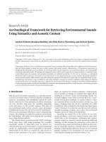
Figure 1: Comparison of detected images based on conventional
approach and hyperspectral approach.
focusing on target detection problems used in surveillance
applications [4].
The rest of this paper is organized as follows. Section 2
describes the background of hyperspec tral signal processing.
The image data structures as well as processing data flow
are descr ibed. We also characterize various key parameters
involved in the detection process. Section 3 discusses detec-

tion characteristics as a function of the bands and libraries.
In Section 4, we present a heuristic band selection strategy.
The algorithm design and the evaluation are discussed in
Section 5,andfinallySection 6 concludes the paper.
2. BACKGROUND AND PROBLEM DESCRIPTION
2.1. Hyperspectral image processing for
detection problems
Consider the problem of detecting flowers in a garden where
a mixture of flowers and various plants are present [5].
Figure 1 illustrates the results where detection based on hy-
perspectral image processing is compared to that of conven-
tional image processing. As show n in Figure 1(a), the object
is detected in conventional image processing with edge detec-
tion using RGB information. Since this image contains many
fragmented detected edges, isolating the desired target image
becomes a challenge [6]. On the other hand, edge detection
can be carried out after the hyperspectral image processing.
TheresultisshowninFigure 1(b) in which only the images
of flowers are detected. Such detection is possible because ev-
ery material has an essential spectral property [7]. In this pa-
per, Figure 1(b) is the ground truth image for comparisons.
Hyperspect ral processing involves three key stages. The
first step is the calibration stage. The image data produced
by a sensor is manipulated to minimize sensor nonunifor-
mity. The sensor is also calibrated by using the initially mea-
sured samples to consider the environment of measurement
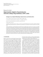
[4, 8]. Each image cube contains a number of bands of spec-
tral contents. For example, the image cube representing the
garden of flowers as shown in Figure 2 consists of 30 bands of
spectral information. Each band represents the information

corresponding to a specific frequency range. Thus, a library
(or spectral information) is constituted by a set of values,
where the number of values corresponds to the number of
Figure 2: Illustration of images corresponding to different bands of
the hyperspectral cube.
bands. In other words, every pixel in the cube is represented
byasetofvalues;thus,atarget(i.e.,objectimagetobede-
tected) is represented by numerous sets of values in a library.
The second step is the detection stage. In the detect ion stage,
target images are detected via isolating the portion of data
which is highly correlated with the given target library. The
target library contains spectral information about the object
intended to be detected. The objective of the detection stage
is to find out the image from the input cube that correlates
with the spectral information stored in the target library. The
third step is the visualization stage which collects detected
image pixels and visualizes through color composition [8].
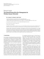
In this paper, we focus our discussion on the detection
stage. Figure 3 illustrates the block diagram of hyperspec-
tral processing. The main challenge of general hyperspectral
image processing is the backside of its advantages: high vol-
ume and complexity of hyperspectral data. The performance
of detection depends on the quality of spectral information
stored in the target library. The main operation in the hy-
perspectral processing for target detection is to compare the
input cube with the target library to determine correlation in
terms of spectra. The detection is based on perceptual seg-
mentation where spectra contents for each subband are cor-
related with the spectra contents stored in the library. How-
ever, not all bands are necessary since some may contain re-

dundant information where they are compared to the tar-
get library. The easiest approach is to reduce the number
of bands and the amount of library for processing. How-
ever, such reduction may eliminate the merit of hyperspec-
tral processing. Hence, one of our objectives is to determine
which bands are effective in detecting the target and selecting
them accordingly. The effectiveness is measured in terms of
the amount of target being detected with a fewer number of
bands. In practice, a perfect target library, which is a set of all
spectr a comprising the target image, does not exist since ob-
jects exhibit different spectral characteristics which are sensi-
tive to environmental factors such as lighting [4, 8, 9]. In the
application of target detection, the basic library is a target
Kyoung-Su Park et al. 3
Calibration
Sensor
calibration table
Sensor Cube data
Sensor non
uniformity
correction
Wave length
calibration
Target
detected
image
Color
composition
Grouping
Gathering

detected
image
Visualization
Detection
Library
Step 0
Load image and
library
Step 3
Correct samples
Step 1
Get correlation
Step 4
Library
refinement
Step 2
Detection
Step 5
Effective band
selection
Figure 3: The block diagram of overall hyperspectral processing. A detailed description of steps is explained in Section 5.
spectrum which is generated in laboratories or measured in
typical environments. Hence, the spectrum of the target im-
age measured by different conditions results in mismatching
the target library. Thus, we propose to refine the target li-
brary dynamically so that effective detection can be achieved
with a small amount of target library information.
2.2. Related work
Traditional store-and-processing system performance is in-
adequate for real-time hyperspectral image processing with-

out data reduction [3]. In this work, a fine-grain, low-
memory and single-instruction multiple-data (SIMD) pro-
cessor is presented as an efficient computational solution for
hyperspectral processing. However, the SIMD processor does
not fully solve the higher resolution and a large number of
band problems.
To minimize the volume of hyperspectral image pro-
cessing, several data compression algorithms are proposed
[10]. They achieve impressive compression ratios but could
lose valuable information for detection or classification even
though the error can be minimized by the clever compression
algorithm.However,overallprocessisaffected by the decom-
pression complexity [11]. Statistical approach based on pat-
tern recognition is one of the solutions for high dimensional-
ity of hyperspectral image processing. It uses a small number
of reference measurements to distinguish material identifica-
tion. However, it requires a large number of sample pixels to
determine accurate probability density function [11].
Even though hyperspectral image processing uses hun-
dreds of bands to detect or classify targets, there is redun-
dancy w hich means that partial bands efficiently accomplish
the edge detection as described in [11, 12]. In [11], the band
selection is based on the band add-on (BAO) procedure that
chooses an initial pair of bands and classifies two spectra by
correlation, and then adds additional bands that increase the
correlation of two spectra. It is a feasible solution to deter-
mine effective bands when an unknown pixel is classified by
using many reference classes. A set of best-bases feature ex-
traction algorithms is proposed for classification of hyper-
spectral data as well [13]. This method is simple, fast, and

highly effective so that it can reduce the input space from
183 dimensions to less than four dimensions in many cases.
However, this approach is based on classification so that it
is suitable when a spectru m of a pixel is classified by many
numbers of libraries. In the application domain of target de-
tection, the input image is compared to a few libraries which
represent the spectrum contents of the target.
2.3. Correlation coefficient of image (A)
Correlation coefficient, A, is a measure of similarity between
the stored spectra in a target library and the obtained spec-
tra from sensors. The high value of correlation indicates the
high degree of similarity between two spectra [14]. The cor-
relation coefficient is defined as
A
= 1 − cos
−1
⎛
⎝

N
T
i=1
t
i
r
i


N
T

i=1
t
2
i


N
T
i=1
r
i
2
⎞
⎠
,(1)
where N
T
is the number of bands in input spectrum, t
i
is the
test spectrum of the ith band, and r
i
is the reference spec-
trum of the ith band. The value of correlation defines a de-
gree of similarity between input spectrum and target spec-
trum stored in the target library.
The input spectra of an object is compared to the spectra
in the target library. This comparison is based on the cor-
relation coefficient. In this paper, we define A
t

as the mini-
mum correlation coefficient value which recognizes the tar-
get between unknown spectra. When the correlation value
is higher than or equal to A
t
, the object is assumed to be
matched with the data in the target library. Thus, the value
is used as an indicator for the degree of confidence in detec-
tion.
If we use lower A
t
to detect targets, it increases the pos-
sibility of wrong detection which means that some back-
grounds are detected as a target. However, if the numbers of
4 EURASIP Journal on Advances in Signal Processing
0
10
20
30
40
50
60
70
80
90
100
Percentage of detected image (P)
0.50.55 0.60.65 0.70.75 0.80.85 0.90.95
1
Minimum correlation coefficient (A

t
)
lib1
lib2
lib3
Tota l
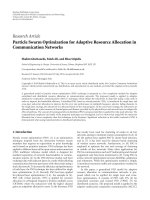
Figure 4: Relationship between the correlation value used and de-
tected image percentage of detected image (P). Thirty one bands of
input image data are used in the simulation.
libraries and bands applied in detection is increased, the per-
formance of target detection is improved. However, even if all
possible information is used to detect targets, there is a limit
value where target and background cannot be isolated. Thus,
the minimum correlation coefficient (A
t
) is related to the
similarity within the target and background. We define A
b
as a maximum correlation value where any correlation value
below A
b
is considered to be a b ackground, which means that
the pixel is not a target at least. The detected image with the
correlation value below A
b
may not be the interest of objects
which may capture a large portion of the background.
2.4. Percentage of detected image (P)
Percentage of detected image (P) shows the effectiveness of
selected bands in the detection process. Figure 4 illustrates

the relationship between the correlation coefficients and per-
centage of detected image (P) where three types of target li-
braries are used. When the given correlation coefficient A
t
is
1, the value of percentage of detected image (P)isverylow
(i.e., approaches zero). For all libraries, when the correla-
tion coefficientisincreased,the percentage of detected image
(P) is decreased. We define A
t
as the correlation value where
the change in percentage of detected image (P) is smaller than
some value δ as we increase the value of the correlation coef-
ficient.
Figure 5 shows the simulation results of the detected im-
age as a function of the minimum correlation values for one
target library, lib1. The detected images are shown for differ-
ent minimum correlation values: 0.70, 0.75, and 0.85. In the
case where A
t
of lib1 is 0.7, unwanted objects that satisfy the
minimum correlation value are detected as a target. However,
as A
t
is increased to 0.85, the unwanted objects almost disap-
pear in the detection at the cost of losing the target image. At
(a) A
t
= 0.7 (b) A
t

= 0.75 (c) A
t
= 0.85
Figure 5: The result of detected image as a function of correlation
values A
t
for lib1. Thirty one input bands are used and processed
with one library.
(a) 2 bands (b) 4 bands (c) 16 bands
Figure 6: The results of detected image as a function of the number
of bands used out of 31 input bands.
the minimum correlation A
t
of 0.85, the process tries to find
only the image from the input that is highly correlated with
the target library.
The values of percentage of detected image (P)havetwo
interpretations. First, the higher value of percentage of de-
tected image ( P) (i.e., more images have been detected) im-
plies that more target images are detected. Second, the higher
value of percentage of detected image (P) can imply that some
of the detected images are not the target. Hence, detection
depends on the number of libraries (spectral information)
and their qualities as well as the minimum correlation values
used in the process.
Under the assumption which multiple libraries are used
in the detection, we define the total percentage of detected
image (P
T
) as follows:

P
T
=

l
P

l, A
t

,(2)
where l is the index of each library and P(l, A
t
) is the per-
centage of detected image (P) value at the correlation value
A
t
when library l is used. We will use the total percentage of
detected image (P) as an indicator for detection performance.
3. TARGET DETECTION
3.1. Effects of number of bands
Since the motivation of our work is to use the smaller num-
ber of bands for detecting the target, we investigate the effects
of the number of bands on detection performance. Thus, the
goal is to minimize the total percentage of detected image (P
T
)
at the minimum correlation (A
t
) given the number of bands

(N
E
).
Kyoung-Su Park et al. 5
0
10
20
30
40
50
60
70
80
90
100
Percentage of detected image (P)
0.50.55 0.60.65 0.70.75 0.80.85 0.90.95 1
Minimum correlation coefficient (A
t
)
lib1
lib2
lib3
Tota l
Figure 7: Relationship between the correlation values and percent-
age of detected image (P) when clustered bands (27, 28, 29, 30) are
used in the detection.
Figure 6 shows the detected image where a partial num-
ber of bands are used to detect flowers. When the number
of bands, N

E
, is equal to 2, the detected image includes the
targetimageaswellasotherunwantedbackgroundimages.
It implies that two bands are not effectively isolating the tar-
get image. When the number of bands is more than 4, the
detected images become isolated and percentage of detected
image (P) is lower than that of the image generated with 2
bands. However, there is only slight improvement (the total
percentage of detected image (P) is decreased) from 4 bands to
16 bands.
We define the degree of effectiveness in terms of the total
percentage of detected image (P
T
). As shown in Figure 6(a), to-
tal percentage of detected image (P
T
) is higher than that shown
in Figures 6(b) and 6(c) (i.e., more images are shown). How-
ever, total percentage of detected image (P
T
)isimproved(re-
duced) very slightly from 4 bands to 16 bands. This shows
that the complete use of the bands is not always necessary for
detecting the target from the input image.
3.2. Redundancy between bands
To use the partial number of bands, the simplest approach is
to select bands in random. In this section, we consider two
types of band selection in order to characterize the effect of
band selection on detection performance. We investigate the
redundancy within the bands.

3.2.1. Clustered bands
Cluster band selection selects N
E
consecutive bands. Figure 7
shows the relationship between the correlation coefficient
and percentage of detected image (P) when 4 consecutive
bands are selected out of 31 possible bands. The selected
(a) With lib1 (b) With lib2 (c) With lib3
(d) Detection with clusters (e) Detected image w ith full
colors
Figure 8: Result of detected image when clustered bands are used
in the detection. Bands used are (27, 28, 29, 30).
bands are (27, 28, 29, 30). The figure shows a much higher
percentage of detected image (P) for the entire range of corre-
lation values when it is compared to that of Figure 4.Thus,
the figure indicates that it has detected more image from the
background. In this situation, it is likely that the detected im-
age contains a lot of unwanted images.
The analysis with the percentage of detected image (P)is
proven by the detected image illustrated in Figure 8.Eachof
the three libraries were not effective in detecting the flowers.
Even with the correlation coefficient of 0.95, the target is not
separated from the background. This simulation suggested
that those clustered bands contain redundancy and the clus-
tered bands are not effective in detecting the target. Similar
results were obtained when the other sets of clusters are used.
Thus, the clustering is not an effective way to select the bands
for detection.
3.2.2. Maximum separation bands
On the other hand, we select the bands that are maximally

separated. There are several combinations of sets of bands.
Figure 9 shows the relationship between correlation and per-
centageofdetectedimage(P) where bands are selected by
maximal separation as (2, 10, 18, 26).
As show n in Figure 9, percentage of detected image (P)val-
uesofeachlibraryaswellasthetotal percentage of detected
image (P
T
) are much lower than that for the entire range
of the correlation values. For example, the total percentage
of detected image (P
T
)ofclusteringcaseatA
t
= 80 is 70
while maximum separation case at A
t
= 80 is 40. This im-
plies that the maximal separation performs better than the
clustering at any minimum correlation value. The detected
image by each library shown in Figure 10 contains only the
flowers. This is improved detection much over the clustering
6 EURASIP Journal on Advances in Signal Processing
0
10
20
30
40
50
60

70
80
90
100
Percentage of detected image (P)
0.50.55 0.60.65 0.70.75 0.80.85 0.90.95 1
Minimum correlation coefficient (A
t
)
lib1
lib2
lib3
Tota l
Figure 9: Relationship between the correlation values and percent-
age of detected image (P) when maximum separation bands are used
in the detection. Band used are (2, 10, 18, 26).
(a) With lib1 (b) With lib3 (c) With lib3
(d) Detection with maximum
separation
(e) Detected image w ith full
colors
Figure 10: Result of detected image when maximum separation
bands are used in the detection. Bands used are (2, 10, 18, 26).
method. Figure 10(d) illustrates the detected image when all
three libraries are used.
However, in the results generated by the maximum sep-
aration, some of the targets were lost. Similar results are
obtained with a different set of bands (4, 12, 20, 28). The
detected images by three target libraries are illustrated in
Figure 11. The band set (4, 12, 20, 28) performs better than

the band set (2, 10, 18, 26) in detecting and isolating the tar-
get images. This implies that while the maximum separation
scheme is better than the clustering, more bands may be nec-
essary since the total percentage of de tected image (P
T
)value
obtained is much higher than the case of 31 bands. We will
present an effective band selection scheme in Section 4.
(a) With lib1 (b) With lib2 (c) With lib3
Figure 11: Result of detected image when maximum separation
bands are used in the detection. Bands used are (4, 12, 20, 28).
3.2.3. Observation
We can observe from the results that detected images are im-
proved when the percentage of detected image (P) value is low
for the given correlation values. This observation coincides
when we compare Figures 4, 7,and9. Percentage of detected
image (P) is the lowest when all bands are used for given
correlation value. We will consider an approach for selecting
bands in the next section.
When the number of bands is increased, percentage of
detected image (P) is reduced and then it is saturated. This
means that a target can be detected by using only partial
bands because some bands have enough information to de-
tect a target.
4. COMPLEXITY REDUCTION STRATEGY
The main objective in reducing computational complexity is
to determine the minimum number of bands used in the de-
tection process as well as selecting a specific set of bands. In
this section, we first define the band contribution coefficient
and present a band selection strategy based on the coefficient.

4.1. Band contribution in detection
Library usually has several spectra for a target because the
spectrum depends on the measurement part of the target
and the condition of light sources. Figure 12 is an example
of spectra for library and background, which shows three li-
braries and two background spectra. When the spectral in-
formation of the target is highly different from the back-
ground, the target detection is easier. In Figure 12, the spec-
trum of lib1 from the 18th band to the 31st band is saturated.
Also, spectrum waveform of lib2 is similar to lib3. However,
the magnitude is different within the two libraries, back-
ground1 is extracted from leaves and background2 is from
the back of a scene.
The effectiveness of the kth band of the lth library, e
l,k
,is
defined as
e
l,k
=



N
B
b=1

l
l,k
− b

b,k



N
B
,(3)
where N
B
is the number of backgrounds, l
l,k
is the kth spec-
trum content in the lth library, and b
b,k
is the kth spectrum
content in the bth background.
Kyoung-Su Park et al. 7
0
50
100
150
200
250
300
Spectrum contents
51015202530
Band index (k)
lib1
lib2
lib3

Background1
Background2
Figure 12: The comparison between spectrum of target libraries
and the spect rum of the background of input bands.
0
20
40
60
80
100
120
Contribution factor (C
k
)
5 1015202530
Band index (k)
Tota l
lib1
lib2
lib3
Figure 13: Illustration of contribution coefficientofeachband.
If a spectrum of a target is similar to that of data in the
library, target detection is achieved more effectively; we will
define the effectiveness as contribution. The contribution co-
efficient (c)isdefinedas
c
k
=

N

lib
l=1
e
l,k
N
lib
,(4)
where c
k
is the contribution of the kth band and N
lib
is the
number of libraries.
The relationship between the contribution factor and the
number of bands is illustrated in Figure 13. Contribution of
lib2 and lib3 is less than 20 while lib1 has much higher con-
tribution than other two libraries. Thus, the contribution of
lib1 is dominant as shown in Figure 13.
Even though the contribution coefficient is not an abso-
lute indicator for detection, the coefficientisconsideredtobe
one of the factors for isolating the target. To obtain the con-
tribution, we need to choose samples of backgrounds. Sam-
ples are randomly selected in a scene, and then each sample
is verified to be a background or an applicant of a target by
using the maximum correlation coefficient (A
b
). If the corre-
lation coefficients between an input spectrum and all of the
libraries are lower than A
b

, the input spectrum is considered
a background. Also, A
b
is experimentally decided depending
on an application. Although background and library can be
highly correlated, the contribution factor is a powerful factor
under the condition of which A
b
is lower than A
t
.
4.2. Effective band selection
Since the contribution coefficient represents the effectiveness
to detect targets, it has a benefit for effective band selection.
However, if the high contribution bands are selected, it may
lead to select clustered bands (i.e., bands 27, 28, 29, 30).
From the definition of correlation in (1), the correla-
tion of library and background is basically the variation
of the difference in two spectra. For example, if the spec-
trum contents in a reference are ( 10, 20, 40, 60, 50, 30) and
the test spectrum has 10 times higher value of contents like
(100, 200, 400, 600, 500, 300), the correlation between two
spectra is 1, which means that two spectra are perfectly cor-
related since the variations of spectrum contents between ad-
jacent bands are the same.
Thus, effective bands represent the variation of differ -
ences between the library and the background. Since contri-
bution is related to the difference between the library and the
background, isolating the target and background in lower A
t

can be one of the solutions in maximally separated bands. To
maximally separate the contribution of selected bands, the
first band has minimum contribution and the last band has
maximum contribution. The contribution of the kth bands is
((max C)
− (min C))/(N
E
− 1) × k +(minC), where (max C)
and (min C) are the values of maximum and minimum con-
tributions, respectively.
For example, let us assume a series of contributions is
(90, 180, 360, 540, 450, 270). Since the contribution of the 1st
band is minimum and the 4th band is maximum, the 1st and
the 4th are selected. Then, since the gap of selected bands
is 150(
= (540 − 90)/3), contributions of second and third
bands are approximately 240 and 390, respectively. Since the
contribution values of the 6th and the 3rd bands are close
to 240 and 390, the 6th and the 3rd bands are selected as ef-
fective bands. Figure 14 shows the result of target detection
when effective bands are selected. The result is similar to the
one in the case where full bands are used.
4.3. Library selection
We have observed that some target libraries work better in
detecting the target than other target libra ries. Theoretically,
a larger set of target libraries will enhance the detection but
at the cost of computational complexity. We investigate the
target library selection in cases where the finite number of
8 EURASIP Journal on Advances in Signal Processing
(a) With lib1 (b) With lib2 (c) With lib3

(d) Detection with effective
band selection
(e) Detected image w ith full
colors
Figure 14: Result of detected image when effective band selection
strategy is used in the detection.
0
10
20
30
40
50
60
70
80
90
100
Percentage of detected image (P)
0.50.55 0.60.65 0.70.75 0.80.85 0.90.95 1
Minimum correlation coefficient (A
t
)
lib1
lib2
lib3
Tota l
Figure 15: Relationship between the correlation values and percent-
age of detected image (P)wheneffective band selection strategy is
used.
target libraries is to be used for reducing the computational

complexity. However, the best possible sets of target libraries
cannot be generated or obtained before the processing. How-
ever, the target library can be improved during the detection
process.
In Figure 15, the total percentage of detected image (P
T
)
from lib1, lib2, and lib3 is 14% when A
t
is equal to 0.8. Even
thoughlib1ismoreeffec tive to detect targets than other li-
braries, lib2 or lib3 can detect the different part of the targets.
Note that the lower value of P
T
does not imply that the
performance is better. It merely suggests that there is a high
0
10
20
30
40
50
60
70
80
90
100
Percentage of detected image (P)
0.50.55 0.60.65 0.70.75 0.80.85 0.90.95 1
Minimum correlation coefficient (A

t
)
lib1
lib2
lib3
Figure 16: Relationship between the correlation values and the per-
centage of detected image (P) when two libraries are used.
probability that the detected image is only a target. Figure 16
shows the relationship between percentage of detected image
(P) and correlation coefficient when it has two libraries (lib2
and lib3). In addition, when several libraries are used, more
effective libraries will produce bigger contributions.
Figure 17 shows the result of target detection where lib2
and lib3 are used. Figures 17(a) and 17(b) have 5.71% and
4.71% of percentage of detected image (P), respectively. Since
the total p ercentage of detected image (P
T
) is 10.39%, two de-
tected areas are slightly overlapped.
4.4. Library refinement
One important aspect that we have discussed in this paper
is that the performance depends on the quality of the target
library. Library refinement improves the detection process.
The overall process starts with a set of basic libraries. Once a
target image is detected, the target library from the detected
image is refined. The refined library has all spectr ums of the
detected target. Once the refined library is generated, the li-
brary is a pplied in lieu of the basic library.
Figure 18 shows the results of library refinement where
the detected image has 0.9 of the correlation coefficient.

Figure 18(a) uses the basic library and Figures 18(b) and
18(c) use the refined library. Since A
t
is not 1 (perfect cor-
relation value), a background image is detected as a target.
Hence, the chosen target image with library refinement is a
candidate of the new library. The randomly selected target
image is compared to the basic library each time. If the cor-
relation between the new library candidate and basic library
satisfies the condition (
≥ A
t
), the current library is replaced
by the new library candidate. Otherwise, the basic library is
used in the process.
In Figure 19, refined libraries are shown by the dashed
line where all refined libraries satisfy the condition of corre-
lation (A
t
= 0.9). The refined library can be adopted in a
variety of light source conditions.
Kyoung-Su Park et al. 9
(a) With lib1 (5.71%) (b) With lib2 (4.71%) (c) With lib1 and lib2
(10.39%)
Figure 17: Library selection.
(a) Basic library (b) Case 1 of refined
library
(c) Case 2 of refined
library
Figure 18: Result of detected images when the libraries are refined from detected samples (A

t
= 0.9).
5. ALGORITHM DESIGN
5.1. Algorithm overview
Figure 20 illustrates the overall algorithm for detecting and
isolating target images in processing where the algorithm has
two processing flows. The right-hand side is for comparing
the input cube with the target libraries. The left-hand side has
two parts where the target library is refined and the effective
band selection is p erformed.
We assume that the basic parameters are loaded in Step 1.
The basic parameters are the number of bands (N
E
), the
number of libraries (N
lib
), the number of background sam-
ples (N
B
) and the number of target samples (N
T
), the mini-
mum correlation coefficient between library and target (A
t
),
and the maximum correlation coefficient between library
and background (A
b
). The basic parameters are based on the
type of the target and detecting environment. The output of

processing is a ser ies of end members which represents a type
of a target.
5.2. Iteration process
The algorithm repeats the following steps until i
= N
x
and
j
= N
y
for a cube.
Step 1. Load spectrum contents in a pixel (i, j) and libraries.
Initially, maximally separated bands are selected as effective
bands. Then, from the next cube, effective bands are selected
by Step 6. Thus, the number of spectrum contents is the same
as the number of effective bands (N
E
).
Step 2. Compute the correlation coefficient between an input
spectrum and the lth library.
Step 3. Classify each pixel (i, j) whether it is a target or a
background; Step 3.1 is for target detection, and Step 3.2 is
for background detection.
Step 3.1. If the correlation coefficient (A) is higher than A
t
,
it is considered to be a target. Even though the libraries are
only for a target, the detected results are saved separately for
library refinement.
Step 3.2. If A is lower than A

b
, it can be a candidate for the
background. Even if a spectrum of a pixel is not considered
to be a target, it can be a target of other libr aries so that there
is a tag bit which takes either false (0) or true value (1). After
the loop for library refinement is completed with tag bit 1, it
is classified as a background.
If the value A is between A
b
and A
t
, it is impossible for the
pixel to be classified due to insufficient information. Thus, to
save end members, N
x
× N
y
× (N
lib
+1)sizeofbitmemo-
ries is required since the area size of x-y plane is N
x
× N
y
and
each end member requires a bit memory to save the informa-
tion where 1 is the end member and 0 is the unknown object.
In addition, since the number of bits to save the type of the
end members in a pixel is the sum of the number of libraries
(N

lib
) and a background, the (N
lib
+ 1) bits are required for
end members. For example, if there are three libraries, the
required end member bits are 4 bits. Furthermore, if all end
member bits are 0 (where background bit is also 0), it is clas-
sified as a background.
Step 4. Choose samples for background and target. To rep-
resent the spectrum of the background area, the samples
of background are randomly selected where the number of
background samples is N
B
. For library refinement, each li-
brary uses one sample as a candidate to replace the current
10 EURASIP Journal on Advances in Signal Processing
0
50
100
150
200
250
300
Spectrum contents
51015202530
Band index (k)
(a) With lib1
0
50
100

150
200
250
300
Spectrum contents
51015202530
Band index (k)
(b) With lib2
Figure 19: The refined libraries of lib1 and lib2 (A
t
= 0.9).
Step 3
Choose target samples (N
T
)
and background samples (N
B
),
l
= 1
Step 4
Get correlation between
a target sample and lth basic
library
Library
refinement
A>A
t
No
Yes

Replace the Library
to basic library
Replace the Library
to target sample
l
= l +1
Get contribution for a library
Step 5
Band
selection
l
= N
lib
No
Yes
Select effective bands
Preprocessing
Step 0
i
= 1, j = 1
load libraries
Load a spectrum of P(i, j)
b
= 0, l = 1
Step 1
Get correlation between
aspectrumandlth library
Step 2a
Yes
A>A

t
No
No
A<A
b
Yes
b
= 0 b = 1
Save as a target
of lib lth
l
= N
lib
No
l
= l +1
Yes
No
b
= 1
Step 2b
Yes
Save as a background
j
= N
y
No
j
= j +1
Yes

i
= N
x
No
i
= i +1,
j
= 1
Yes
Postprocessing
Figure 20: Flowchart of proposed algorithm for the detection process.
Kyoung-Su Park et al. 11
Step 0
Step 1
Step 2
Step 3
Step 4
Step 5
detect(
·)
corr(
·)
(1, 1)load(
·)
init(
·)
T
pixel
(2, 1)
T

cube
(N
x
, N
y
)
choose
samples(·)
refine
lib(·)
get
ebands(·)
Figure 21: Time flow in processing.
0
2
Execution time (s/cube)
N
E
= 4 N
E
= 8 N
E
= 16 N
E
= 32
The number of effective bands
Step 1
Step 2
Step 3
Step 4

Step 5
Step 6
(a) N
E
0
2
Execution time (s/cube)
N
lib
= 3 N
lib
= 6 N
lib
= 12 N
lib
= 24
The number of libraries
Step 1
Step 2
Step 3
Step 4
Step 5
Step 6
(b) N
lib
Figure 22: The execution time in function of number of effective bands and the number of libraries, where (a) N
lib
= 3, N
x
= 820, N

y
= 748,
N
B
= 1000, N
T
= 1000; (b) N
E
= 4, N
x
= 820, N
y
= 748, N
B
= 1000, N
T
= 1000.
library. We assume the area of targets is much smaller
than the area of background. All of the detected targets are
counted and randomly selected in endmembers. If we count
all backgrounds to select randomly, they make excessive data
loading so that we select N
B
random pixels from the entire
image.
Step 5. Refine c urrent library. The sample is a candidate for
the new library. Since the partial number of bands is used to
obtain correlation in Steps 2 and 3, the sample is compared
to the basic library again for entire bands. If A is higher than
A

t
where the correlation between the lth library and a spec-
trum of a sample uses all of the bands of which size is N
z
, the
candidate replaces the current library. Otherwise, the current
library goes back to the basic librar y. The refined librar y is
saved to a memory for libraries.
Step 6. Select effective bands. From Step 5, we obtained the
new library so that effective bands are changed to support
the new library. Since the band selection is based on contr i-
bution, (N
lib
× N
B
) operations are required to get contribu-
tion (c). From the distribution of contribution coefficient,
N
E
bands are selected.
Figure 21 shows the timing flow of hyperspectral process-
ing algorithm. T
init
represents the time interval for loading
libraries and several coefficients such as the minimum corre-
lation coefficient between library and input image (A
t
), the
12 EURASIP Journal on Advances in Signal Processing
0

2
Execution time (s/cube)
N
B
= 1000 N
B
= 2000 N
B
= 4000 N
B
= 8000
The number of background samples
Step 1
Step 2
Step 3
Step 4
Step 5
Step 6
(a) N
B
0
2
Execution time (s/cube)
N
T
= 1000 N
T
= 2000 N
T
= 4000 N

T
= 8000
The number of target samples
Step 1
Step 2
Step 3
Step 4
Step 5
Step 6
(b) N
T
Figure 23: The execution time in function of number of background samples or the number of target samples, where (a) N
E
= 4, N
lib
= 3,
N
x
= 820, N
y
= 748, N
T
= 1000; (b) N
E
= 4, N
lib
= 3, N
x
= 820, N
y

= 748, N
B
= 1000.
maximum correlation coefficient between a library and an
input image (A
b
), the number of libraries (N
lib
), the num-
ber of target samples (N
T
), the number of background sam-
ples (N
B
), and the number of effective bands (N
E
). T
pixel
is
the processing time for a pixel and the sum of T
load
, T
corr
and T
detect
from Step 1 to Step 3,whereT
load
is the required
time for the function load(
·)inStep 1, T

corr
is for the func-
tion corr(
·)inStep 2,andT
detect
is the required time for
the function detect(
·)inStep 3. Thus, the total required
time for a cube is T
init
+ T
pixel
× N
x
× N
y
+ T
choose samples
+
T
refine lib
+ T
get ebands
,whereT
choose samples
is the required time
for the function choose
samples(·)inStep 4, T
refine lib
is for

the function of refine
lib(·)inStep 5,andT
get ebands(·)
is the
required time for the func tion get
ebands(·)inStep 6.
5.3. Complexity
The complexity of this algorithm has been estimated by
TMS320C6713 (300 MHz) based on the VLIW architecture.
The internal program memory is structured so that a total of
eight instructions can be fetched in every cycle [15, 16]. We
estimate the execution time from the instruction cycle count
using Code Composer Studio 3.1.
Figure 22(a) shows the execution time in terms of the
number of bands used. The complexity of the system is di-
rectly related to the execution time. When the number of ef-
fective bands is increased, the complexity as well as the exe-
cution time are increased.
The computation complexity in terms of the number of
target libraries is shown in Figure 22(b). The increasing rate
of complexity is higher than the case shown in Figure 22(a)
since the complexity of Step 3 is also increased as the number
of libraries is increased.
The band selection is based on the relationship between
backgrounds and libraries. The background samples rep-
resent the background area. Thus, the number of back-
ground samples is important for the effective band selection.
Figure 23(a) shows the complexity in terms of the number of
background samples. When the number of background sam-
ples is larger, the complexity of Steps 4 and 6 is increased.

However, the total computation complexity is slightly in-
creased.
The number of target samples is important for library
refinement since the sample represents the detected image.
Figure 23(b) shows the variation of computation complexity
in terms of the number of background samples.
Kyoung-Su Park et al. 13
6. CONCLUSION
This paper has presented spectra l characterization for effi-
cient image detection using hyperspectral processing tech-
niques. We proposed an algorithm to reduce complexity and
improve the library by using effective band selection and li-
brary refinement. The effective bands are heur istically se-
lected for processing based on the contribution coefficient
defined in this paper. The complexity of the proposed algo-
rithm has been estimated in TMS320C6713 DSP. This ap-
proach has reduced the computation complexity. We have
shown that for effective detection, only a small number of
bands are needed.
ACKNOWLEDGMENT
This research is supported by the Ubiquitous Computing
and Network (UCN) Project, the Ministry of Information
and Communication (MIC) 21st Century Frontier R&D Pro-
gram in Korea.
REFERENCES
[1] T.BoggsandR.B.Gomez,“Fasthyperspectraldataprocess-
ing methods,” in Geo-Spatial Image and Data Exploitation II,
vol. 4383 of Proceedings of SPIE, pp. 74–78, Orlando, Calif,
USA, April 2001.
[2] R.B.GomezandA.J.Lewis,“On-boardprocessingforspec-

tral remote sensing,” in ISPRS Special Session Future Intelligent
Earth Observing Satellites (FIEOS ’02),Denver,Colo,USA,
November 2002.
[3] S. M. Chai, A. Gentile, W. E. Lugo-Beauchamp, J. Fonseca, J. L.
Cruz-Rivera, and D. S. Wills, “Forcal-plane processing archi-
tectures for real-time hyperspectral image processing,” Applied
Optics, vol. 39, no. 5, pp. 835–849, 2000.
[4] G. A. Shaw and H. K. Burke, “Spectral imaging for remote
sensing,” Lincoln Laboratory Journal, vol. 14, no. 1, pp. 3–28,
2003.
[5] S.M.C.Nascimento,F.P.Ferreira,andD.H.Foster,“Statistics
of spatial cone-excitation ratios in natural scenes,” Journal of
the Optical Society of America A, vol. 19, no. 8, pp. 1484–1490,
2002.
[6]R.C.GonzalezandR.E.Woods,Digital Image Processing,
Prentice-Hall, Upper Saddle River, NJ, USA, 2nd edition, 2002.
[7] W. H. Bakker and K. S. Schmidt, “Hyperspectral edge filter-
ing for measuring homogeneity of surface cover types,” ISPRS
Journal of Photogrammetry and Remote Sensing,vol.56,no.4,
pp. 246–256, 2002.
[8] M. L. Nischan, R. M. Joseph, J. C. Libby, and J. P. Kerekes,
“Active spectral imaging,” Lincoln Laboratory Journal, vol. 14,
no. 1, pp. 131–144, 2003.
[9] M. K. Griffin and H. K. Burke, “Compensation of hyperspec-
tral data for atmospheric effects,” Lincoln Laboratory Journal,
vol. 14, no. 1, pp. 29–54, 2003.
[10] G. P. Abousleman, M. W. Marcellin, and B. R. Hunt, “Hyper-
spectral image compression using entropy-constrained pre-
dictive trellis coded quantization,” IEEE Transactions on Image
Processing, vol. 6, no. 4, pp. 566–573, 1997.

[11] N. Keshava, “Distance metrics and band selection in hyper-
spectral processing with applications to material identification
and spectral libraries,” IEEE Transactions on Geoscience and Re-
mote Sensing, vol. 42, no. 7, pp. 1552–1565, 2004.
[12] P. Bajcsy and P. Groves, “Methodology for hyperspectral band
selection,” Photogrammetric Engineering and Remote Sensing,
vol. 70, no. 7, pp. 793–802, 2004.
[13] S. Kumar, J. Ghosh, and M. M. Crawford, “Best-bases feature
extraction algorithms for classification of hyperspectral data,”
IEEE Transactions on Geoscience and Remote Sensing, vol. 39,
no. 7, pp. 1368–1379, 2001.
[14] G. Girouard, A. Bannari, A. Harti, and A. Desrochers, “Val-
idated spectral angle mapper algorithm for geological map-
ping: comparative study between quickbird and landsat-tm,”
in The 20th International Society for Photogrammetry and Re-
mote Sensing Congress, pp. 599–605, Istanbul, Turkey, July
2004.
[15] R. Chassaing, Digital Signal Processing and Applications with
the C6713 and C6416 DSK, John Wiley & Sons, New York, NY,
USA, 2005.
[16] Texas Instrument, “Datasheet of TMS320C6713B,” November
2005, />Kyoung-Su Park received B.S. and M.S. de-
grees in electrical engineering from Chon-
buk National University, South Korea, in
1999 and 2001, respectively, and M.S. de-
gree in electrical and computer engineering
from Stony Brook University – State Uni-
versity of New York in 2005. He is currently
pursuing the Ph.D. degree at Stony Brook
University. He was with Research Center of

Hyosung Corporation, South Korea, from
2001 to 2002, where he was an RF Circuit and System Designer.
His research interests include circuits for image processing and ar-
chitecture optimization for high-performance DSP systems design.
Sangjin Hong received the B.S. and M.S.
degrees in electrical engineering and com-
puter science degree from the University of
California, Berkeley. He received his Ph.D.
in electrical engineering and computer sci-
ence degree from the University of Michi-
gan, Ann Arbor. He is currently with the
Department of Electrical and Computer
Engineering at State University of New
York, Stony Brook. Before joining SUNY, he
has worked at Ford Aerospace Corp. Computer Systems Division
as a Systems Engineer. He also worked at Samsung Electronics in
Korea as a Technical Consultant. His current research interests are
in the areas of low-power VLSI design of multimedia wireless com-
munications and digital signal processing systems, reconfigurable
SoC design and optimization, VLSI signal processing, and low-
complexity dig ital circuits. He served on numerous technical pro-
gram committees for IEEE conferences. He is a Senior Member of
IEEE.
Peom Park is a Professor in the Department
of Industrial and Information Systems En-
gineering, Ajou University, Suwon, South
Korea, also he is serving as Chief Execu-
tive Officer in HuminTec Co., Ltd. He got
a Ph.D. degree from Iowa State University
and worked in ETRI Electronics, Inc. in Ko-

rea. His research area is human-computer
interaction in the applied IT technology
with telemedicine, telematics, and ubiqui-
tous lifecare system.
14 EURASIP Journal on Advances in Signal Processing
We-Duke Cho received a B.S. degree in 1981
from Sogang University, and his M.S. and
Ph.D. degrees from Korea Advanced Insti-
tute of Science and Technology (KAIST) in
1983 and 1987. Currently, he is a Profes-
sor at the Department of Electronics Engi-
neering College of Information Technology
at Ajou University in South Korea. His re-
search interests included ubiquitous com-
puting/network, sensor network, post-PC
(next generation PC smart PDA), interactive DTV broadcasting
technology, high-level home server and gateway, digital broadcast-
ing and mobile convergence platform technology, and wireless net-
work.