Báo cáo hóa học: " Research Article Sequential Monte Carlo Methods for Joint Detection and Tracking of Multiaspect Targets in Infrared Radar Images" pptx

Hindawi Publishing Corporation
EURASIP Journal on Advances in Signal Processing
Volume 2008, Article ID 217373, 13 pages
doi:10.1155/2008/217373
Research Article
Sequential Monte Carlo Methods for Joint Detec tion and
Tracking of Multiaspect Targets in Infrared Radar Images
Marcelo G. S. Bruno, Rafael V. Ara
´
ujo, and Anton G. Pavlov
Instituto Tecnol
´
ogico de Aeron
´
autica, S
˜
ao Jos
´
e dos Campos, SP 12228, Brazil
Correspondence should be addressed to Marcelo G. S. Bruno,
Received 30 March 2007; Accepted 7 August 2007
Recommended by Yvo Boers
We present in this paper a sequential Monte Carlo methodology for joint detection and tracking of a multiaspect target in im-
age sequences. Unlike the traditional contact/association approach found in the literature, the proposed methodology enables
integrated, multiframe target detection and tracking incorporating the statistical models for target aspect, target motion, and
background clutter. Two implementations of the proposed algorithm are discussed using, respectively, a resample-move (RS) par-
ticle filter and an auxiliary particle filter (APF). Our simulation results suggest that the APF configuration outperforms slightly the
RS filter in scenarios of stealthy targets.
Copyright © 2008 Marcelo G. S. Bruno et al. This is an open access article distributed under the Creative Commons Attribution
License, which permits unrestricted use, distribution, and reproduction in any medium, provided the original work is properly
cited.

1. INTRODUCTION
This paper investigates the use of sequential Monte Carlo fil-
ters [1] for joint multiframe detection and tracking of ran-
domly changing multiaspect targets in a sequence of heavily
cluttered remote sensing images generated by an infrared air-
borne radar (IRAR) [2]. For simplicity, we restrict the discus-
sion primarily to a single target scenario and indicate briefly
how the proposed algorithms could be modified for multi-
object tracking.
Most conventional approaches to target tracking in im-
ages [3] are based on suboptimal decoupling of the detection
and tracking tasks. Given a reference target template, a two-
dimensional (2D) spatial matched filter is applied to a single-
frame of the image sequence. The pixel locations where the
output of the matched filter exceeds a pre-specified threshold
are treated then as initial estimates of the true position of de-
tected targets. Those preliminary position estimates are sub-
sequently assimilated into a multiframe tracking algorithm,
usually a linearized Kalman filter, or alternatively discarded
as false alarms originating from clutter.
Depending on its level of sophistication, the spatial
matched filter design might or might not take into account
the spatial correlation of the background clutter and random
distortions of the true target aspect compared to the refer-
ence template. In any case, however, in a scenario with dim
targets in heavily cluttered environments, the suboptimal as-
sociation of a single-frame matched filter detector and a mul-
tiframe linearized tracking filter is bound to perform poorly
[4].
As an alternative to the conventional approaches, we in-

troduced in [5, 6] a Bayesian algorithm for joint multiframe
detection and tracking of known targets, fully incorporat-
ing the statistical models for target motion and background
clutter and overcoming the limitations of the usual associ-
ation of single-frame correlation detectors and Kalman fil-
ter trackers in scenarios of stealthy targets. An improved ver-
sion of the algorithm in [5, 6] was later introduced in [7]
to enable joint detection and tracking of targets with un-
known and randomly changing aspect.The algorithms in [5–
7] were however limited by the need to use discrete-valued
stochastic models for both target motion and target aspect
changes, with the “absent target” hypothesis treated as an ad-
ditional dummy aspect state. A conventional hidden Markov
model (HMM) filter was used then to perform joint min-
imum probability of error multiframe detection and maxi-
mum a posteriori (MAP) tracking for targets that were de-
clared present in each frame. A smoothing version of the
joint multiframe HMM detector/tracker, based essentially
on a 2D version of the forward-backward (Baum-Welch)
2 EURASIP Journal on Advances in Signal Processing
algorithm, was later proposed in [4]. Furthermore, we also
proposed in [4] an alternative tracker based on particle fil-
tering [1, 8] which, contrary to the original HMM tracker in
[7], assumed a continuous-valued kinematic (position and
velocity) state and a discrete-valued target aspect state. How-
ever, the particle filter algorithm in [4] enabled tracking only
(assuming that the target was always present in all frames)
and used decoupled statistically independent models for tar-
get motion and target aspect.
To better capture target motion, we drop in this paper

the previous constraint in [5–7] and, as in the later sections
of [4], allow the unknown 2D position and velocity of the
target to be continuous-valued random variables. The un-
known target aspect is still modeled however as a discrete
random variable defined on a finite set I, where each sym-
bol is a pointer to a possibly rotated, scaled, and/or sheared
version of the target’s reference template. In order to inte-
grate detection and tracking, building on our previous HMM
work in [7], we extend the set I to include an additional
dummy state that represents the absence of a target of interest
in the scene. The evolution over time of the target’s kinematic
and aspect states is described then by a coupled stochastic dy-
namic model where the sequences of target positions, veloc-
ities, and aspects are mutually dependent.
Contrary to alternative feature-based trackers in the liter-
ature, the proposed algorithm in this paper detects and tracks
the target directly from the raw sensor images, processing
pixel intensities only. The clutter-free target image is modeled
by a nonlinear function that maps a given target centroid po-
sition into a spatial distribution of pixels centered around the
(quantized) centroid position, with shape and intensity being
dependent on the current target aspect. Finally, the target is
superimposed to a structured background whose spatial cor-
relation is captured by a noncausal Gauss-Markov random
field (GMRf) model [9–11]. The GMRf model parameters
are adaptively estimated from the observed data using an ap-
proximate maximum likelihood (AML) algorithm [12].
Given the problem setup described in the previous pa
ragraph, the optimal solution to the integrated detection/
tracking problem requires the recursive computation at each

frame n of the joint posterior distribution of the target’s kine-
matic and aspect states conditioned on all observed frames
from instant 0 up to instant n. Given, however, the inherent
nonlinearity of the observation and (possibly) motion mod-
els, the exact computation of that posterior distribution is
generally not possible. We resort then to mixed-state parti-
cle filtering [13] to represent the joint posterior by a set of
weighted samples (or particles) such that, as the number of
particles goes to infinity, their weighted average converges (in
some statistical sense) to the desired minimum mean-square
error (MMSE) estimate of the hidden states. Following a se-
quential importance sampling (SIS) [14] approach, the par-
ticles may be drawn recursively from the coupled prior statis-
tical model for target motion and aspect, while their respec-
tive weights may be updated recursively using a likelihood
function that takes into account the models for the target’s
signature and for the background clutter.
We propose two different implementations for the
mixed-state particle filter detector/tracker. The first imple-
mentation, which was previously discussed in a conference
paper (see [15]) is a resample-move (RS) filter [16] that uses
particle resampling [17] followed by a Metropolis-Hastings
move step [18] to combat both particle degeneracy and par-
ticle impoverishment (see [8]). The second implementation,
which was not included in [15], is an auxiliary particle filter
(APF) [19] that uses the current observed frame at instant n
to preselect those particles at instant n
−1 which, when prop-
agated through the prior dynamic model, are more likely to
generate new samples with high likelihood. Both algorithms

are original with respect to the previous particle filtering-
based tracking algorithm that we proposed in [4], where the
problem of joint detection and tracking with coupled motion
and aspect models was not considered.
Related work and different approaches in the literature
Following the seminal work by Isard and Blake [20], parti-
cle filters have been extensively applied to the solution of vi-
sual tracking problems. In [21], a sequential Monte Carlo al-
gorithm is proposed to track an object in video subject to
model uncertainty. The target’s aspect, although unknown,
is assumed, however, to be fixed in [21], with no dynamic
aspect change. On the other hand, in [22], an adaptive ap-
pearance model is used to specify a time-varying likelihood
function expressed as a Gaussian mixture whose parameters
are updated using the EM [23] algorithm. As in our work,
the algorithm in [22] also processes image intensities di-
rectly, but, unlike our problem setup, the observation model
in [22] does not incorporate any information about spatial
correlation of image pixels, treating instead each pixel as in-
dependent observations. A different Bayesian algorithm for
tracking nonrigid (randomly deformable) objects in three-
dimensional images using multiple conditionally indepen-
dent cues is presented in [24]. Dynamic object appearance
changes are captured by a mixed-state shape model [13]con-
sisting of a discrete-valued cluster membership parameter
and a continuous-valued weight parameter. A separate kine-
matic model is used in turn to describe the temporal evolu-
tion of the object’s position and velocity. Unlike our work,
the kinematic model in [24] is assumed statistically indepen-
dent of the aspect to model.

Rather than investigating solutions to the problem of
multiaspect tracking of a single target, several recent ref-
erences, for example, [25, 26], use mixture particle filters
to tackle the different but related problem of detecting and
tracking an unknown number of multiple objects with dif-
ferent but fixed appearance. The number of terms in the
nonparametric mixture model, that represents the posterior
of the unknowns, is adaptively changed as new objects are
detected in the scene and initialized with a new associated
observation model. Likewise, the mixture weights are also
recursively updated from frame to frame in the image se-
quence.
Organization of the paper
The paper is divided into 6 sections. Section 1 is this in-
troduction. In Section 2, we present the coupled model
MarceloG.S.Brunoetal. 3
for target aspect and motion and review the observation
and clutter models focusing on the GMRf representation of
the background and the derivation of the associated likeli-
hood function for the observed (target + clutter) image. In
Section 3, we detail the proposed detector/tracker in the RS
and APF configurations. The performance of the two filters
is discussed in Section 4 using simulated infrared airborne
radar (IRAR) data. A preliminary discussion on multitarget
tracking is found in Section 5,followedbyanillustrativeex-
ample with two targets. Finally, we present in Section 6 the
conclusions of our work.
2. THE MODEL
In the sequel, we present the target and clutter models that
are used in this paper. We use lowercase letters to denote both

random variables/vectors and realizations (samples) of ran-
dom variables/vectors; the proper interpretation is implied
in context. We use lowercase p to denote probability den-
sity functions (pdfs) and uppercase P to denote the probabil-
ity mass functions (pmfs) of discrete random variables. The
symbol Pr(A) is used to denote the probability of an event A
in the σ-algebra of the sample space.
State variables
Let n be a nonnegative integer number and let superscript
T denote the transpose of a vector or matrix. The kine-
matic state of the target at frame n is defined as the four-
dimensional continuous (real-valued) random vector s
n
=
[
x
n
˙
x
n
y
n
˙
y
n
]
T
, that collects the positions, x
n
and y

n
,and
the velocities,
˙
x
n
and
˙
y
n
, of the target’s centroid in a system
of 2D Cartesian coordinates (x, y). On the other hand, the
target’s aspect state at frame n,denotedbyz
n
,isassumedto
be a discrete random variable that takes values in the finite
set I
={0, 1,2, 3, , K}, where the symbol “0” is a dummy
state that denotes that the target is absent at frame n,and
each symbol i, i
= 1, , K, is in turn a pointer to one possi-
bly rotated, scaled, and/or sheared version of the target’s ref-
erence template.
2.1. Target motion and aspect models
The random sequence
{(s
n
, z
n
)}, n ≥ 0, is modeled as first-

order Markov process specified by the pdf of the initial kine-
matic state p(s
0
), the transition pdf p(s
n
| z
n
, s
n−1
, z
n−1
),
the transition probabilities Pr(
{z
n
= i}|{z
n−1
= j}, s
n−1
),
(i, j)
∈ I×I, and the initial probabilities Pr({z
0
= i}), i ∈ I.
Aspect change model
Assume that, at any given frame, for any aspect state z
n
, the
clutter-free target image lies within a bounded rectangle of
size (r

i
+ r
s
+1)× (l
i
+ l
s
+ 1). In this notation, r
i
and r
s
de-
note the maximum pixel distances in the target image when
we move away, respectively, up and down, from the target
centroid. Analogously, l
i
and l
s
are the maximum horizon-
tal pixel distances in the target image when we move away,
respectively, left and right, from the target centroid.
Assume also that each image frame has the size of L
×M
pixels. We introduce next the extended grid

L ={(r,j):−r
s
+
1
≤ r ≤ L +r

i
, −l
s
+1≤ j ≤ M + l
i
} that contains all possible
target centroid locations for which at least one target pixel
still lies in the sensor image. Next, let G be a matrix of size
K
×K such that G(i, j) ≥ 0foranyi, j = 1, 2, , K and
K

i=1
G(i, j) = 1 ∀j = 1, , K. (1)
Assuming that a transition from a “present target” state to the
“absent target” state can only occur when the target moves
out of the image, we model the probability of a change in the
target’s aspect from the state j to the state i,Pr(
{z
n
= i}|
{
z
n−1
= j}, s
n−1
), as
G(i, j)Pr

s

∗
n
∈

L

| s
n−1
,

z
n−1
= j

, i, j = 1, , K,
1
−Pr

s
∗
n
∈

L

| s
n−1
,

z

n−1
= j

, i = 0, j
/
=0,
p
a
K
, i
/
=0, j = 0,
1
− p
a
, i = 0, j = 0,
(2)
where the two-dimensional vector s
∗
n
= (x
∗
n
, y
∗
n
) denotes the
quantized target centroid position defined on the extended
image grid and obtained from the four-dimensional contin-
uous kinematic state s

n
by making
x
∗
n
= round

x
n
ζ
1

,
y
∗
n
= round

y
n
ζ
2

,
(3)
where ζ
1
and ζ
2
are the spatial resolutions of the image, re-

spectively, in the directions x and y. The parameter p
a
in
(2) denotes in turn the probability of a new target enter-
ing the image once the previous target became absent. For
simplicity, we restrict the discussion in this paper to the sit-
uation where there is at most one single target of interest
present in the scene at each image frame. The specification
Pr(
{z
n
= i}|{z
n−1
= 0}, s
n−1
) = p
a
/K, i = 1, , K,corre-
sponds to assuming the worst-case scenario where, given that
a new target entered the scene, there is a uniform probability
that the target will take any of the K possible aspect states.
Finally, the term 1
−Pr({s
∗
n
∈

L}|s
n−1
, {z

n−1
= j})in(2)is
the probability of a target moving out of the image at frame
n given its kinematic and aspect states at frame n
−1.
Motion model
For simplicity, we assume that, except in the situation
where there is a transition from the “absent target” state
to the “present target” state, the conditional pdf p(s
n
|
z
n
, s
n−1
, z
n−1
) is independent of the current and previous as-
pect states, respectively, z
n
and z
n−1
. In other words, unless
z
n−1
= 0andz
n
/
=0, we make
p


s
n
| z
n
, s
n−1
, z
n−1

= f
s

s
n
| s
n−1

,(4)
4 EURASIP Journal on Advances in Signal Processing
where f
s
(s
n
| s
n−1
) is an arbitrary pdf (not necessarily Gaus-
sian) that models the target motion. Otherwise, if z
n−1
= 0

and z
n
/
=0, we reset the target’s position and make
p

s
n
| z
n
, s
n−1
, z
n−1

=
f
0

s
n

,(5)
where f
0
(s
n
) is typically a noninformative (e.g., uniform)
prior pdf defined in a certain region (e.g., upper-left corner)
of the image grid. Given the independence assumption in (4),

it follows that, for any j
= 1, , K,
Pr

s
∗
n
∈

L

| s
n−1
,

z
n−1
= j

=

{s
n
|s
∗
n
∈

L}
f

s

s
n
| s
n−1

ds
n
.
(6)
2.2. Observation model and likelihood function
Next, we discuss the target observation model. Previous ref-
erences mentioned in Section 1,forexample,[21, 22, 24–26],
are concerned mostly with video surveillance of near objects
(e.g., pedestrian or vehicle tracking), or other similar appli-
cations (e.g., face tracking in video). For that class of applica-
tions, effects such as object occlusion are important and must
be explicitly incorporated into the target observation model.
In this paper by contrast, the emphasis is on a different ap-
plication, namely, detection and tracking of small, quasipoint
targets that are observed by remote sensors (usually mid-to
high-altitude airborne platforms) and move in highly struc-
tured, generally smooth backgrounds (e.g., deserts, snow-
covered fields, or other forms of terrain). Rather than mod-
eling occlusion, our emphasis is instead on additive natural
clutter.
Image frame model
Assuming a single target scenario, the nth frame in the image
sequence is modeled as the L

×M matrix:
Y
n
= H(s
∗
n
, z
n
)+V
n
,(7)
where the matrix V
n
represents the background clutter and
H(s
∗
n
, z
n
) is a nonlinear function that maps the quantized tar-
get centroid position, s
∗
n
= (x
∗
n
, y
∗
n
), (see (3)) into a spatial

distribution of pixels centered at s
∗
n
and specified by a set of
deterministic and known target signature c oefficients depen-
dent on the aspect state z
n
. Specifically, we make [4]
H

x
∗
n
, y
∗
n
, z
n

=
r
s

k=−r
i
l
s

l=−l
i

a
k,l

z
n

E
x
∗
n
+k,y
∗
n
+l
,(8)
where E
g,t
is an L × M matrixwhoseentriesareallequalto
zero, except for the element (g, t) which is equal to 1.
For a given fixed template model z
n
= i ∈ I, the co-
efficients
{a
k,l
(i)} in (8) are the target signature coefficients
responding to that particular template. The signature coeffi-
cients are the product of a binary parameter b
k,l
(z

n
) ∈ B =
{
0, 1}, that defines the target shape for each aspect state, and
arealcoefficient φ
k,l
(s
n
) ∈ R, that specifies the pixel intensi-
ties of the target, again for the various states in the alphabet I.
For simplicity, we assume that the pixel intensities and shapes
are deterministic and known at each frame for each possible
value of z
n
.Inparticular,ifz
n
takes the value 0 denoting ab-
sence of target, then the function H(:, :) in (7) reduces to the
identically zero matrix, indicating that sensor observations
consist of clutter only.
Remark 1. Equation (8) assumes that the target’s template
is entirely located within the sensor image grid. Otherwise,
for targets that are close to the image borders, the summa-
tion limits in (8) must be changed accordingly to take into
account portions of the target that are no longer visible.
Clutter model
In order to describe the spatial correlation of the background
clutter, we assume that, after suitable preprocessing to re-
move the local means, the random field V
n

(r, j), 1 ≤ r ≤ L,
1
≤ j ≤ M, is modeled as a first-order noncausal Gauss-
Markov random field (GMrf) described by the finite differ-
ence equation [9]
V
n
(r, j) = β
c
v,n

V
n
(r −1, j)+V
n
(r +1,j)

+ β
c
h,n

V
n
(r, j − 1) + V
n
(r, j +1)

+ ε
n
(r, j),

(9)
where E
{V
n
(r, j)ε
n
(k,l)}=σ
2
c,n
δ
r−k, j−l
,withδ
i,j
= 1ifi = j
and zero otherwise. The symbol E
{·}denotes here the expec-
tation(orexpectedvalue)ofarandomvariable/vector.
Likelihood function model
Let y
n
, h(s
∗
n
, z
n
), and v
n
be the one-dimensional equiva-
lent representations, respectively, of Y
n

, H(s
∗
n
, z
n
)andV
n
in
(7), obtained by row-lexicographic ordering. Let also Σ
v
=
E[v
n
v
T
n
] denote the covariance matrix associated with the
random vector v
n
, assumed to have zero mean after appro-
priate preprocessing. For a GMrf model as in (9), the corre-
sponding likelihood function for a fixed aspect state z
n
= z,
z ∈{1,2, 3, , K},isgivenby[4]
p

y
n
| s

n
, z

= p

y
n
| s
n
,0

exp

2λ(s
n
, z ) −ρ(s
n
, z )
2σ
2
c,n

(10)
where
λ

s
n
, z


= y
T
n

σ
2
c,n
Σ
−1
v

h

s
∗
n
, z

(11)
is referred to in our work as the data term and
ρ

s
n
, z

= h
T

s

∗
n
, z

σ
2
c,n
Σ
−1
v

h

s
∗
n
, z

(12)
is called the energ y term. On the other hand, for z
n
= 0,
p(y
n
| s
n
, z
n
) reduces to the likelihood of the absent target
state, which corresponds to the probability density function

of y
n
assuming that the observation consists of clutter only,
that is,
p(y
n
| s
n
,0)=
1
(2π)
LM/2

det

Σ
v

1/2
exp

−
1
2
y
T
n
Σ
−1
v

y
n

.
(13)
MarceloG.S.Brunoetal. 5
Writing the difference equation (9) in compact matrix
notation, it can be shown [9–11] by the application of the
principle of orthogonality that Σ
−1
v
has a block-tridiagonal
structure of the form
σ
2
c,n
Σ
−1
v
= I
L
⊗

I
M
−β
c
h,n
B
M


+ B
L
⊗

−β
c
v,n
I
M

, (14)
where
⊗ denotes the Kronecker product, I
J
is J × J identity
matrix, and B
J
is a J ×J matrix whose entries B
J
(k,l) = 1if
|k − l|=1 and are equal to zero otherwise.
Using the block-banded structure of Σ
−1
v
in (14), it can be
further shown that λ(s
n
, z ) may be evaluated as the output of
a modified 2D spatial matched filter using the expression

λ(s
n
, z ) =
r
s

k=−r
i
l
s

l=−l
i
a
k,l
(z )d(s
∗
n
(1) + k, s
∗
n
(2) + l), (15)
where s
∗
n
(i), i = 1, 2, are obtained, from (3), and d(r, j) is the
output of a 2D differential operator
d(r, j)
= Y
n

(r, j) −β
c
h,n

Y
n
(r, j − 1) + Y
n
(r, j +1)

−
β
c
v,n

Y
n
(r −1, j)+Y
n
(r +1,j)

(16)
with Dirichlet (identically zero) boundary conditions.
Similarly, the energy term ρ(s
n
, z ) can be also efficiently
computed by exploring the block-banded structure of Σ
−1
v
.

The resulting expression is the difference between the au-
tocorrelation of the signature coefficients
{a
k,l
} and their
lag-one cross-correlations weighted by the respective GMrf
model parameters β
c
h,n
or β
c
v,n
. Before we leave this section,
we make two additional remarks.
Remark 2. As before, (15)isvalidforr
i
+1≤ s
∗
n
(1) ≤ L − r
s
and l
i
+1 ≤ s
∗
n
(2) ≤ M−l
s
. For centroid positions close to the
image borders, the summation limits in (15)mustbevaried

accordingly (see [6] for details).
Remark 3. Within our framework, a crude non-Bayesian sin-
gle frame maximum likelihood target detector could be built
by simply evaluating the likelihood map p(y
n
| s
n
, z
n
)for
each aspect state z
n
and finding the maximum over the image
grid of the sum of likelihood maps weighted by the a priori
probability for each state z
n
(usually assumed to be identical).
A target would be considered present then if the weighted
likelihood peak exceeded a certain threshold. In that case, the
likelihood peak would also provide an estimate for the target
location. The integrated joint detector/tracker presented in
Section 3 outperforms, however, the decoupled single-frame
detector discussed in this remark by fully incorporating the
dynamic motion and aspect motion into the detection pro-
cess and enabling multiframe detection within the context of
a track-before-detect philosophy.
3. PARTICLE FILTER DETECTOR/TRACKER
3.1. Sequential importance sampling
Given a sequence of observed frames
{y

1
, , y
n
},ourgoal
is to generate, at each instant n, a properly weighted set of
samples (or particles)
{s
(j)
n
, z
(j)
n
}, j = 1, , N
p
, with associ-
ated weights
{w
(j)
n
} such that, according to some statistical
criterion, as N
p
goes to infinity,
N
p

j=1
w
(j)
n



s
(j)
n

T
z
(j)
n

T
−→ E

s
T
n
z
n

T
| y
1:n

. (17)
A possible mixed-state sequential importance sampling (SIS)
strategy (see [4, 13]) for the recursive generation of the par-
ticles
{s
(j)

n
, z
(j)
n
} and their proper weights is described in the
algorithm below.
(1) Initialization For j
= 1, , N
p
(i) Draw s
(j)
0
∼p(s
0
), and z
(j)
0
∼P(z
0
).
(ii) Make w
(j)
0
= 1/N
p
and n = 1.
(2) Importance Sampling For j = 1, , N
p
(i) Draw z
(j)

n
∼P(z
n
| z
(j)
n
−1
, s
(j)
n
−1
) according to (2).
(ii) Draw
s
(j)
n
∼p(s
n
| z
(j)
n
, s
(j)
n
−1
, z
(j)
n
−1
) according to (4)or

(5).
(iii) Update the importance weights
w
(j)
n
∝ w
(j)
n
−1
p

y
n
| s
(j)
n
, z
(j)
n

(18)
using the likelihood function in Section 2.2.
End-For
(i) Normalize the weights
{w
(j)
n
} such that

N

p
j=1
w
(j)
n
= 1.
(ii) For j
=1, , N
p
,makes
(j)
n
=s
(j)
n
, z
(j)
n
=z
(j)
n
,andw
(j)
n
=

w
(j)
n
.

(iii) Make n
= n +1andgobacktostep2.
3.2. Resample-move filter
The sequential importance sampling algorithm in Section
3.1 is guaranteed to converge asymptotically with probability
one; see [27]. However, due to the increase in the variance of
the importance weights, the raw SIS algorithm suffers from
the “particle degeneracy” phenomenon [8, 14, 17]; that is,
after a few steps, only a small number of particles will have
normalized weights close to one, whereas the majority of the
particles will have negligible weight. As a result of particle de-
generacy, the SIS algorithm is inefficient, requiring the use of
a large number of particles to achieve adequate performance.
Resampling step
A possible approach to mitigate degeneracy is [17]tore-
sample from the existing particle population with replace-
ment according to the particle weights. Formally, after
the normalization of importance weights
{w
(j)
n
},wedraw
i
(j)
∼{1, 2, , N
p
}with Pr({i
(j)
= l}) = w
(l)

n
, and build a new
particle set
{
s
(j)
n
,
z
(j)
n
}, j = 1, , N
p
, such that (
s
(j)
n
,
z
(j)
n
) =
(s
(i
(j)
)
n
, z
(i
(j)

)
n
). After the resampling step, the new selected tra-
jectories (
s
(j)
0:n
,
z
(j)
0:n
) = (s
(i
(j)
)
0:n
−1
,s
(i
(j)
)
n
, z
(i
(j)
)
0:n
−1
, z
(i

(j)
)
n
) are approx-
imately distributed (see, e.g., [28]) according to the mixed
6 EURASIP Journal on Advances in Signal Processing
posterior pdf p(s
0:n
, z
0:n
| y
1:n
) so that we can reset all parti-
cle weights to 1/N
p
.
Move step
Although particle resampling according to the weights re-
duces particle degeneracy, it also introduces an undesir-
able side effect, namely, loss of diversity in the particle
population as the resampling processes generate multiple
copies of a small number or, in the extreme case, only one
high-weight particle. A possible solution, see [16], to re-
store sample diversity without altering the sample statis-
tics is to move the current particles
{
s
(j)
n
,

z
(j)
n
} to new lo-
cations
{s
(j)
n
, z
(j)
n
} using a Markov chain transition kernel
k(s
(j)
n
, z
(j)
n
| s
(j)
n
, z
(j)
n
), that is, invariant to the conditional
mixture pdf p(s
n
, z
n
|

s
(j)
0:n
−1
,
z
(j)
0:n
−1
, y
1:n
). Provided that the
invariance condition is satisfied, the new particle trajecto-
ries (s
(j)
0:n
, z
(j)
0:n
) = (
s
(j)
0:n
−1
, s
(j)
n
,
z
(j)

0:n
−1
, z
(j)
n
) remain distributed
according to p(s
0:n
, z
0:n
| y
1:n
) and the associated particle
weights may be kept equal to 1/N
p
. A Markov chain that sat-
isfies the desired invariance condition can be built using the
following Metropolis-Hastings strategy [15, 18].
For j
= 1, , N
p
, the following algorithm holds.
(i) Draw
z
(j)
n
∼P(z
n
|
z

(j)
n
−1
,
s
(j)
n
−1
) according to (2).
(ii) Draw
s
(j)
n
∼p(s
n
| z
(j)
n
,
s
(j)
n
−1
,
z
(j)
n
−1
) according to (4)or
(5).

(iii) Draw u
∼U([0, 1]).
If
u
≤ min

1,
p

y
n
| s
(j)
n
, z
(j)
n

p

y
n
|
s
(j)
n
,
z
(j)
n



, (19)
then

s
(j)
n
, z
(j)
n

=


s
(j)
n
, z
(j)
n

. (20)
Else,

s
(j)
n
, z
(j)

n

=

s
(j)
n
,
z
(j)
n

. (21)
(iv) Reset w
(j)
n
= 1/N
p
.
End-For.
3.3. Auxiliary particle filter
An alternative to the resample-move filter in Section 3.2 is to
use the current observation y
n
to preselect at instant n − 1a
set of particles that, when propagated to instant n according
to the system dynamics, is more likely to generate samples
with high likelihood. That can be done using an auxiliary
particle filter (APF) [19] which samples in two steps from
a mixed importance function:

q

i, s
n
, z
n
| y
1:n

∝ w
(i)
n
−1
p

y
n
| s
(i)
n
, z
(i)
n

p

s
n
, z
n

| s
(i)
n
−1
z
(i)
n
−1

,
(22)
where
z
(j)
n
and s
(j)
n
are drawn according to the mixed prior
p(s
n
, z
n
| s
(j)
n
−1
, z
(j)
n

−1
). The proposed algorithm is summarized
into the following steps.
(1) Pre-sampling Selection Step For j
= 1, , N
p
(i) Draw z
(j)
n
∼P(z
n
| z
(j)
n
−1
, s
(j)
n
−1
) according to (2).
(ii) Draw
s
(j)
n
∼p(s
n
| z
(j)
n
, s

(j)
n
−1
, z
(j)
n
−1
) according to (4)or
(5).
(iii) Compute the first-stage importance weights
λ
(j)
n
∝ w
(j)
n
−1
p

y
n
| s
(j)
n
, z
(j)
n

,
N

p

j=1
λ
(j)
n
= 1, (23)
using the likelihood function model in Section 2.2.
End-For
(2) Importance Sampling with Auxiliary Particles For j
=
1, , N
p
(i) Sample i
(j)
∼{1, , N
p
} with Pr({i
(j)
= l}) = λ
(l)
n
.
(ii) Sample
z
(j)
n
∼P(z
n
| z

(i
(j)
)
n
−1
, s
(i
(j)
)
n
−1
) according to (2).
(iii) Sample
s
(j)
n
∼p(s
n
| z
(j)
n
, s
(i
(j)
)
n
−1
, z
(i
(j)

)
n
−1
) according to (4)or
(5).
(iv) Compute the second-stage importance weights
w
(j)
n
∝
p

y
n
| s
(j)
n
, z
(j)
n

p

y
n
| s
(i
(j)
)
n

, z
(i
(j)
)
n

. (24)
End-For.
(v) Normalize the weights
{w
(j)
n
} such that

N
p
j=1
w
(j)
n
= 1.
(3) Post-sampling Selection Step For j
= 1, , N
p
(i) Draw k
(j)
∼{1, , N
p
} with Pr({k
(j)

= l}) = w
(l)
n
.
(ii) Make s
(j)
n
= s
(k
(j)
)
n
z
(j)
n
= z
(k
(j)
)
n
and w
(j)
n
= 1/N
p
.
End-For.
(iii) Make n
= n +1andgobacktostep1.
3.4. Multiframe detector/tracker

The final result at instant n of either the RS algorithm in
Section 3.2 or the APF algorithm in Section 3.3 is a set of
equally weighted samples
{s
(j)
n
, z
(j)
n
} that are approximately
distributed according to the mixed posterior p(s
n
, z
n
| y
1:n
).
Next, let H
1
denote the hypothesis that the target of interest
is present in the scene at frame n. Conversely, let H
0
denote
the hypothesis that the target is absent. Given the equally
weighted set
{s
(j)
n
, z
(j)

n
}, we compute then the Monte Carlo
estimate,

Pr({z
n
= 0}|y
1:n
), of the posterior probability of
target absence by dividing the number of particles for which
z
(j)
n
= 0 by the total number of particles N
p
. The minimum
probability of error test to decide between hypotheses H
1
and
H
0
at frame n is approximated then by the decision rule

Pr

z
n
= 0

| y

1:n
)
H
0
≷
H
1
1 −

Pr(

z
n
= 0

| y
1:n

(25)
MarceloG.S.Brunoetal. 7
or, equivalently,

Pr

z
n
= 0

|
y

1:n

H
0
≷
H
1
1
2
. (26)
Finally, if H
1
is accepted, the estimate s
n|n
of the target’s
kinematic state at instant n is obtained from the Monte Carlo
approximation of E[s
n
| y
1:n
, {z
n
/
=0}], which is computed
by averaging out the particles s
(j)
n
such that z
(j)
n

/
=0.
4. SIMULATION RESULTS
In this section, we quantify the performance of the proposed
sequential Monte Carlo detector/tracker, both in the RS and
APF configurations, using simulated infrared airborne radar
(IRAR) data. The background clutter is simulated from real
IRAR images from the MIT Lincoln Laboratory database,
available at the CIS website, at Johns Hopkins University.
An artificial target template representing a military vehicle
is added to the simulated image sequence. The simulated
target’s centroid moves in the image from frame to frame
according to the simple white-noise acceleration model in
[3, 4] with parameters q
= 6andT = 0.04 second. A total
of four rotated, scaled, or sheared versions of the reference
template is used in the simulation.
The target’s aspect changes from frame to frame follow-
ing a known discrete-valued hidden Markov chain model
where the probability of a transition to an adjacent aspect
state is equal to 40%. In the notation of Section 2.1, that
specification corresponds to setting G(1, 1)
= G(4, 4) = 0.6,
G(2, 2)
= G(3, 3) = 0.2, G(i, j) = 0.4if|i − j|=1, and
G(i, j)
= 0 otherwise. All four templates are equally likely at
frame zero, that is, P(z
0
) = 1/4forz

0
= 1, 2, 3,4. The initial
x and y positions of the target’s centroid at instant zero are
assumed to be uniformly distributed, respectively, between
pixels 50 and 70 in the x coordinate and pixels 10 and 20 in
the y coordinate. The initial velocities v
x
and v
y
are in turn
Gaussian-distributed with identical means (10 m/s or 2 pix-
els/frame) and a small standard deviation (σ
= 0.1).
Finally, the background clutter for the moving target se-
quence was simulated by adding a sequence of synthetic
GMrf samples to a matrix of previously stored local means
extracted from the database imagery. The GMrf samples were
synthetized using correlation and prediction error variance
parameters estimated from real data using the algorithms de-
veloped in [11, 12]see[4]foradetailedpseudocode.
Two video demonstrations of the operation of the pro-
posed detector/tracker are available for visualization by click-
ing on the links in [29]. The first video (peak target-to-clutter
ratio, or PTCR
≈ 10 dB) illustrates the performance over 50
frames of an 8 000-particle RS detector/tracker implemented
as in Section 3.2, whereas the second video (PTCR
≈ 6.5 dB)
demonstrates the operation over 60 frames of a 5 000-particle
APF detector/tracker implemented as in Section 3.3.Both

video sequences show a target of interest that is tracked in-
side the image grid until it disappears from the scene; the
algorithm then detects that the target is absent and correctly
indicates that no target is present. Next, once a new target en-
120
100
80
60
40
20
20 40 60 80 100 120
(a)
120
100
80
60
40
20
20 40 60 80 100 120
(b)
Figure 1: (a) First frame of the cluttered target sequence, PTCR =
10.6 dB; (b) target template and position in the first frame shown as
a binary image.
ters the scene, that target is acquired and tracked accurately
until, in the case of the APF demonstration, it leaves the scene
and no target detection is once again correctly indicated.
Both video demos show the ability of the proposed al-
gorithms to (1) detect and track a present target both inside
the image grid and near its borders, (2) detect when a target
leaves the image and indicate that there is no target present

until a new target appears and (3), when a new target enters
the scene, correctly detect that the target is present and track
it accurately. In the sequel, for illustrative purposes only, we
show in the paper the detection/tracking results for a few se-
lected frames using the RS algorithm and a dataset that is
different from the one shown in the video demos.
Figure 1(a) shows the initial frame of the sequence with
the target centered in the (quantized) coordinates (65, 23)
and superimposed on clutter. The clutter-free target tem-
plate, centered at the same pixel location, is shown as a binary
image in Figure 1(b). The simulated PTCR in Figure 1(b) is
10.6 dB.
8 EURASIP Journal on Advances in Signal Processing
120
100
80
60
40
20
20 40 60 80 100 120
(a)
120
100
80
60
40
20
20 40 60 80 100 120
(b)
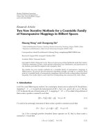
Figure 2: (a) Tenth frame of the cluttered target sequence, PTCR =

10.6 dB, with target translation, rotation, scaling, and shearing; (b)
target template and position in the tenth frame shown as a binary
image.
Next, Figure 2(a) shows the tenth frame in the image se-
quence. Once again, we show in Figure 2(b) the correspond-
ing clutter-free target image as a binary image. Note that the
target from frame 1 has now undergone a random change in
aspect in addition to translational motion.
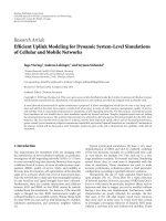
The tracking results corresponding to frames 1 and 10 are
shown, respectively, in Figures 3(a) and 3(b). The actual tar-
get positions are indicated by a cross sign (’+’), while the es-
timated positions are indicated by a circle (’o’). Note that the
axes in Figures 1(a) and 1(b) and Figures 2(a) and 2(b) rep-
resent integer pixel locations, while the axes in Figures 3(a)
and 3(b) represent real-valued x and y, coordinates assum-
ing spatial resolutions of ξ
1
= ξ
2
= 0.2 meters/pixel such
that the [0, 120] pixel range in the axes of Figures 1(a) and
1(b) and Figures 2(a) and 2(b) corresponds to a [0, 24] me-
ter range in the axes of Figures 3(a) and 3(b).
In this particular example, the target leaves the scene at
frame 31 and no target reappears until frame 37. The SMC
25
20
15
10
5

0
+
o
0 5 10 15 20 25
(a)
25
20
15
10
5
0
+
o
0 5 10 15 20 25
(b)
Figure 3: Tracking results: actual target position (+), estimated tar-
get position (o); (a) initial frame, (b) tenth frame.
tracker accurately detects the instant when the target dis-
appears and shows no false alarms over the 6 absent target
frames as illustrated in Figures 4(a) and 4(b) where we show,
respectively, the clutter+background-only thirty-sixth frame
and the corresponding tracking results indicating in this case
that no target has been detected. Finally, when a new target
reappears, it is accurately acquired by the SMC algorithm.
The final simulated frame with the new target at position
(104, 43) is shown for illustration purposes in Figure 5(a).
Figure 5(b) shows the corresponding tracking results for the
same frame.
In order to obtain a quantitative assessment of track-
ing performance, we ran 100 independent Monte Carlo sim-

ulations using, respectively, the 5000-particle APF detec-
tor/tracker and the 8000-particle RS detector/tracker. Both
algorithms correctly detected the presence of the target over a
sequence of 20 simulated frames in all 100 Monte Carlo runs.
However, with PTCR
= 6.5 dB, the 5000-particle APF tracker
MarceloG.S.Brunoetal. 9
120
100
80
60
40
20
20 40 60 80 100 120
(a)
25
20
15
10
5
0
No target detected
0 5 10 15 20 25
(b)
Figure 4: (a) Thirty-sixth frame of the cluttered target sequence
with no target present; (b) detection result indicating absence of
target.
diverged (i.e., failed to estimate the correct target trajectory)
in 3 out of the 100 Monte Carlo trials, whereas the RS tracker
diverged in 5 out of 100 runs. When we increased the PTCR

to 8.1 dB, the divergence rates fell to 2 out of 100 for the APF,
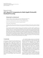
and 3 out of 100 for the RS filter. Figures 6(a) and 6(b) show,
in the case of PTCR
= 6.5 dB, the root mean square (RMS)
error curves (in number of pixels) for the target’s position
estimates, respectively, in coordinates x and y generated by
both the APF and the RS trackers. The RMS error curves in
Figure 6 were computed from the estimation errors recorded
in each of the 100 Monte Carlo trials, excluding the divergent
realizations. Our simulation results suggest that, despite the
reduction in the number of particles from 8000 to 5000, the
APF tracker still outperforms the RS tracker, showing similar
RMS error performance with a slightly lower divergence rate.
For both filters, in the nondivergent realizations, the estima-
tion error is higher in the initial frames and decreases over
time as the target is acquired and new images are processed.
120
100
80
60
40
20
20 40 60 80 100 120
(a)
25
20
15
10
5
0

+
o
0 5 10 15 20 25
(b)
Figure 5: (a) Fifty-first frame of the cluttered target sequence,
PTCR
= 10.6 dB, with a new target present in the scene; (b) tracking
results: actual target position (+), estimated target position (o).
5. PRELIMINARY DISCUSSION ON
MULTITARGET TRACKING
We have considered so far a single target with uncertain as-
pect (e.g., random orientation or scale). In theory, however,
the same modeling framework could be adapted to a sce-
nario where we consider multiple targets with known (fixed)
aspect. In that case, the discrete state z
n
, rather than repre-
senting a possible target model, could denote instead a pos-
sible multitarget configuration hypothesis. For example, if
we knew a priori that there is a maximum of N
T
targets in
the field of view of the sensor at each time instant, then z
n
would take K = 2
N
T
possible values corresponding to the
hypotheses ranging from “no target present” to “all targets
present” in the image frame at instant n. The kinematic state

s
n
, on the other hand, would have variable dimension de-
pending on the value assumed by z
n
, as it would collect the
centroid locations of all targets that are present in the image
10 EURASIP Journal on Advances in Signal Processing
0
0.2
0.4
0.6
0.8
1
1.2
1.4
RMSE (number of pixels)
0 5 10 15 20
Frame number
Auxiliary particle filter, N
p
= 5000
Resample-move filter, N
p
= 8000
(a)
0.2
0.4
0.6
0.8

1
1.2
RMSE (number of pixels)
0 5 10 15 20
Frame number
Auxiliary particle filter, N
p
= 5000
Resample-move filter, N
p
= 8000
(b)
Figure 6: RMS error for the target’s position estimate, respectively,
for the APF (divergence rate, 3%) and resample-move (divergence
rate,5%)trackers,PTCR
= 6.5 d; (a) x coordinate, (b) y coordinate.
given a certain target configuration hypothesis. Different tar-
gets could be assumed to move independently of each other
when present and to disappear only when they move out of
the target grid as discussed in Section 2. Likewise, a change in
target configuration hypotheses would result in new targets
appearing in uniformly random locations as in (5).
The main difficulty associated with the approach de-
scribed in the previous paragraph is however that, as the
number of targets increases, the corresponding growth in the
dimension of the state space is likely to exacerbate particle
depletion, thus causing the detection/tracking filters to di-
verge if the number of particles is kept constant. That may
render the direct application of the joint detection/tracking
algorithms in this paper unfeasible in a multitarget scenario.

The basic tracking routines discussed in the paper may be still
viable though when used in conjunction with more conven-
tional algorithms for target detection/acquisition and data
association. For a review of alternative approaches to mul-
titarget tracking, mostly for video applications, we refer the
reader to [30–33].
5.1. Likelihood function modification in
a multitarget scenario
In the alternative scenario with multiple (at most N
T
) targets,
where z
n
represents one of 2
N
T
possible target configurations,
the likelihood function model in (10) depends instead on a
sum of data terms
λ
n,i

s
n
, z
n

=
y
T

n

σ
2
c,n
Σ
−1
v

h
i

s
n
, z
n

,1≤ i ≤ 2
N
T
, (27)
andasumofenergyterms
ρ
i,j

s
n
, z
n


=
h
T
i

s
n
, z
n

σ
2
c,n
Σ
−1
v

h
j

s
n
, z
n

,1≤ i, j ≤ 2
N
T
,
(28)

where h
i
(s
n
, z
n
) is the long-vector representation of the
clutter-free image of the ith target under the target configu-
ration hypothesis z
n
, assumed to be identically zero for target
configurations under which the ith target is not present. The
sum of the data terms corresponds to the sum of the out-
puts of different correlation filters matched to each of the N
T
possible (fixed) target templates taking into account the spa-
tial correlation of the clutter background. The energy terms,
ρ
i,j
(s
n
, z
n
), are on the other hand constant with s
n
for most
possible locations of targets i and j on the image grid, except
when either one of the two targets or both are close to the
image borders. Finally, for i
/

= j, the energy terms are zero for
present targets that are sufficiently apart from each other and,
therefore, most of the time, they do not affect the computa-
tion of the likelihood function. The terms ρ
i,j
(s
n
, z
n
)mustbe
taken into account, however, for overlapping targets; in this
case, they may be computed efficiently exploring the sparse
structure of h
i
and Σ
−1
v
. For details, we refer the reader to
future work.
5.2. Illustrative example with two targets
We conclude this preliminary discussion on multitarget
tracking with an illustrative example where we track two sim-
ulated targets moving on the same real clutter background
from Section 4 for 22 consecutive frames. This example dif-
fers, however, from the simulations in Section 4 in the sense
that, rather than performing joint detection and tracking
of the two targets, the algorithm assumes a priori that two
targets are always present in the scene and performs target
tracking only. The two targets are preacquired (detected) in
the initial frame such that their initial positions are known

up only to a small uncertainty. For this particular simula-
tion, with PTCR
≈ 12.5 dB, that preliminary acquisition was
MarceloG.S.Brunoetal. 11
120
100
80
60
40
20
20 40 60 80 100 120
(a)
120
100
80
60
40
20
20 40 60 80 100 120
(b)
Figure 7: Simulated image sequence with two moving targets: (a)
first frame, (b) tenth frame; PTCR
≈ 12.5 dB.
done by applying the differential filter in (16) to the initial
frame, and then applying the output of the differential filter
to a bank of two spatial matched filters as in (15), designed
according to the signature coefficients, respectively, for tar-
gets 1 and 2. The outputs of the two matched filters minus
the corresponding energy terms for targets 1 and 2, respec-
tively, are finally added together and thresholded to provide

the initial estimates of the location of the two targets. Note
that the cross-energy terms discussed in Section 5.1 may be
ignored in this case since we are assuming that the two tar-
gets are initially sufficiently far apart. Frames 1 and 10 of the
simulated cluttered sequence with the two targets are shown
in Figures 7(a) and 7(b) for illustration purposes.
Once the two targets are initially acquired, we track them
jointly from the raw sensor images (i.e., without any other
conventional decoupled data association/tracking method)
using an auxiliary particle filter that assumes the modified
likelihood function of Section 5.1 and two independent mo-
tion models, respectively, for targets 1 and 2. The tracking
filter uses N
p
= 8 000 particles. Figure 8 shows the actual
20
30
40
50
60
70
Pixel location (y coordinate)
40 60 80 100 120
Pixel location (x coordinate)
Actual T1
Actual T2
Estimated T1
Estimated T2
Figure 8: Illustrative example of two-target tracking using an aux-
iliary particle filter.

and estimated trajectories, respectively, for targets 1 and 2.
As we can see from the plots, the experimental results are
worse than those obtained in the single target, multiaspect
case, but the filter was still capable of tracking the pixel loca-
tions of the centroids of the two targets fairly accurately with
errors ranging from zero to two or three pixels at most and
without using any ad hoc data association routine.
6. CONCLUSIONS AND FUTURE WORK
We discussed in this paper a methodology for joint detection
and tracking of multiaspect targets in remote sensing image
sequences using sequential Monte Carlo (SMC) filters. The
proposed algorithm enables integrated, multiframe target de-
tection and tracking incorporating the statistical models for
target motion, target aspect, and spatial correlation of the
background clutter. Due to the nature of the application, the
emphasis is on detecting and tracking small, remote targets
under additive clutter, as opposed to tracking nearby objects
possibly subject to occlusion.
Two d i fferent implementations of the SMC detec-
tor/tracker were presented using, respectively, a resample-
move (RS) particle filter and an auxiliary particle filter (APF).
Simulation results show that, in scenarios with heavily ob-
scured targets, the APF and RS configurations have similar
tracking performance, but the APF algorithm has a slightly
smaller percentage of divergent realizations. Both filters, on
the other hand, were capable of correctly detecting the target
in each frame, including accurately declaring absence of tar-
get when the target left the scene and, conversely, detecting
a new target when it entered the image grid. The multiframe
track-before-detect approach allowed for efficient detection

of dim targets that may be near invisible in a single-frame
but become detectable when seen across multiple frames.
12 EURASIP Journal on Advances in Signal Processing
The discussion in this paper was restricted to targets that
assume only a finite number of possible aspect states defined
on a library of target templates. As an alternative for future
work, an appearance model similar to the one described in
[24] could be used instead, allowing the discrete-valued as-
pect states s
n
to denote different classes of continuous-valued
target deformation models, as opposed to fixed target tem-
plates. Similarly, the framework in this paper could also be
modified to allow for multiobject tracking as indicated in
Section 5.
ACKNOWLEDGMENT
Part of the material in this paper was presented at the 2005
IEEE Aerospace Conference.
REFERENCES
[1] A. Doucet, S. Godsill, and C. Andrieu, “On sequential Monte
Carlo sampling methods for Bayesian filtering,” Statistics and
Computing, vol. 10, no. 3, pp. 197–208, 2000.
[2] J. K. Bounds, “The Infrared airborne radar sensor suite,” RLE
Tech. Rep. 610, Massachusetts Institute of Technology, Cam-
bridge, Mass, USA, December 1996.
[3] Y. Bar-Shalom and X. Li, Multitarget-Multisensor Tracking:
Principles and Techniques, YBS Publishing, Storrs, Conn, USA,
1995.
[4] M. G. S. Bruno, “Bayesian methods for multiaspect target
tracking in image sequences,” IEEE Transactions on Signal Pro-

cessing, vol. 52, no. 7, pp. 1848–1861, 2004.
[5] M.G.S.BrunoandJ.M.F.Moura,“Optimalmultiframede-
tection and tracking in digital image sequences,” in Proceedings
of the IEEE International Acoustics, Speech, and Signal Process-
ing (ICASSP ’00), vol. 5, pp. 3192–3195, Istanbul, Turkey, June
2000.
[6]M.G.S.BrunoandJ.M.F.Moura,“Multiframede-
tector/tracker: optimal performance,” IEEE Transactions on
Aerospace and Electronic Systems, vol. 37, no. 3, pp. 925–945,
2001.
[7]M.G.S.BrunoandJ.M.F.Moura,“MultiframeBayesian
tracking of cluttered targets with random motion,” in Pro-
ceedings of the International Conference on Image Processing
(ICIP ’00), vol. 3, pp. 90–93, Vancouver, BC, Canada, Septem-
ber 2000.
[8] M.S.Arulampalam,S.Maskell,N.Gordon,andT.Clapp,“A
tutorial on particle filters for online nonlinear/non-Gaussian
Bayesian tracking,” IEEE Transactions on Signal Processing,
vol. 50, no. 2, pp. 174–188, 2002.
[9] J. M. F. Moura and N. Balram, “Recursive structure of non-
causal Gauss-Markov random fields,” IEEE Transactions on In-
formation Theory, vol. 38, no. 2, pp. 334–354, 1992.
[10] J. M. F. Moura and M. G. S. Bruno, “DCT/DST and Gauss-
Markov fields: conditions for equivalence,” IEEE Transactions
on Signal Processing, vol. 46, no. 9, pp. 2571–2574, 1998.
[11] J. M. F. Moura and N. Balram, “Noncausal Gauss Markov ran-
dom fields: parameter structure and estimation,” IEEE Trans-
actions on Information Theory, vol. 39, no. 4, pp. 1333–1355,
1993.
[12] S. M. Schweizer and J. M. F. Moura, “Hyperspectral imagery:

clutter adaptation in anomaly detection,” IEEE Transactions on
Information Theory, vol. 46, no. 5, pp. 1855–1871, 2000.
[13] M. Isard and A. Blake, “A mixed-state condensation tracker
with automatic model-switching,” in Proceedings of the 6th In-
ternational Conference on Computer Vision, pp. 107–112, Bom-
bay, India, January 1998.
[14] A. Doucet, J. F. G. Freitas, and N. J. Gordon, “An introduc-
tion to sequential Monte Carlo methods,” in Sequential Monte
Carlo Methods in Practice, A. Doucet, N. F. G. Freitas, and N.
J. Gordon, Eds., Springer, New York, NY, USA, 2001.
[15] M.G.S.Bruno,R.V.deAra
´
ujo, and A. G. Pavlov, “Sequential
Monte Carlo filtering for multi-aspect detection/tracking,” in
Proceedings of the IEEE Aerospace Conference, pp. 2092–2100,
Big Sky, Mont, USA, March 2005.
[16] W. R. Gilks and C. Berzuini, “Following a moving target—
Monte Carlo inference for dynamic Bayesian models,” Journal
of the Royal Statistical Society: Series B (Statistical Methodol-
ogy), vol. 63, no. 1, pp. 127–146, 2001.
[17] N. Gordon, D. Salmond, and C. Ewing, “Bayesian state esti-
mation for tracking and guidance using the bootstrap filter,”
Journal of Guidance, Control, and Dynamics,vol.18,no.6,pp.
1434–1443, 1995.
[18] C. P. Robert and G. Casella, Monte Carlo Statistical Meth-
ods, Springer Texts in Statistics, Springer, New York, NY, USA,
1999.
[19] M. K. Pitt and N. Shephard, “Filtering via simulation: auxil-
iary particle filters,” Journal of the American Statistical Associa-
tion

, vol. 94, no. 446, pp. 590–599, 1999.
[20] M. Isard and A. Blake, “Condensation—conditional density
propagation for visual tracking,” International Journal of Com-
puter Vision, vol. 29, no. 1, pp. 5–28, 1998.
[21] B. Li and R. Chellappa, “A generic approach to simultaneous
tracking and verification in video,” IEEE Transactions on Image
Processing, vol. 11, no. 5, pp. 530–544, 2002.
[22] S. K. Zhou, R. Chellappa, and B. Moghaddam, “Visual track-
ing and recognition using appearance-adaptive models in par-
ticle filters,” IEEE Transactions on Image Processing, vol. 13,
no. 11, pp. 1491–1506, 2004.
[23] A. P. Dempster, N. M. Laird, and D. B. Rubin, “Maximum like-
lihood from incomplete data via the EM algorithm,” Journal of
the Royal Statistical Society: Series B (Statistical Methodology),
vol. 39, no. 1, pp. 1–38, 1977.
[24] J. Giebel, D. M. Gavrila, and C. Schn
¨
orr, “A bayesian frame-
work for multi-cue 3D object tracking,” in Proceedings of
the 8th European Conference on Computer Vision (ECCV ’04),
vol. 4, pp. 241–252, Prague, Czech Republic, May 2004.
[25] J. Vermaak, A. Doucet, and P. P
´
erez, “Maintaining multi-
modality through mixture tracking,” in Proceedings of the 9th
IEEE International Conference on Computer Vision (ICCV ’03),
vol. 2, pp. 1110–1116, Nice, France, October 2003.
[26] K. Okuma, A. Taleghani, N. de Freitas, J. J. Little, and D.
G. Lowe, “A boosted particle filter: multitarget detection and
tracking,” in Proceedings of the 8th European Conference on

Computer Vision (ECCV ’04), vol. 3021, pp. 28–39, Prague,
Czech Republic, May 2004.
[27] J. Geweke, “Bayesian inference in econometric models using
Monte Carlo integration,” Econometrica,vol.57,no.6,pp.
1317–1339, 1989.
[28] J. S. Liu, R. Chen, and T. Logvinenko, “A theoretical frame-
work for sequential importance sampling with resampling,” in
Sequential Monte Carlo Methods in Practice,A.Doucet,J.F.G.
Freitas, and N. J. Gordon, Eds., pp. 225–246, Springer, New
York, NY, USA, 2001.
[29] Video Demonstration 1 & 2, />∼bruno.
MarceloG.S.Brunoetal. 13
[30] W. Ng, J. Li, S. Godsill, and J. Vermaak, “Tracking variable
number of targets using sequential Monte Carlo methods,” in
Proceedings of the IEEE/SP 13th Workshop on Stat istical Signal
Processing, pp. 1286–1291, Bordeaux, France, July 2005.
[31] W. Ng, J. Li, S. Godsill, and J. Vermaak, “Multitarget tracking
using a new soft-gating approach and sequential Monte Carlo
methods,” in Proceedings of the IEEE International Conference
on Acoustics, Speech, and Signal Processing (ICASSP ’05), vol. 4,
pp. 1049–1052, Philadelphia, Pa, USA, March 2005.
[32]C.Hue,J P.LeCadre,andP.P
´
erez, “Tracking multiple ob-
jects with particle filtering,” IEEE Transactions on Aerospace
and Electronic Systems, vol. 38, no. 3, pp. 791–812, 2002.
[33] J. Czyz, B. Ristic, and B. Macq, “A color-based particle filter for
joint detection and tracking of multiple objects,” in Proceed-
ingd of the IEEE International Conference on Acoustics, Speech,
and Signal Processing (ICASSP ’05), pp. 217–220, Philadelphia,

Pa, USA, March 2005.