Báo cáo hóa học: " Research Article Clock Estimation for Long-Term Synchronization in Wireless Sensor Networks with Exponential Delays" docx

Hindawi Publishing Corporation
EURASIP Journal on Advances in Signal Processing
Volume 2008, Article ID 219458, 6 pages
doi:10.1155/2008/219458
Research Article
Clock Estimation for Long-Term Synchronization in
Wireless Sensor Networks with Exponential Delays
Qasim M. Chaudhari and Erchin Serpedin
Department of Electrical and Computer Engineering, Texas A&M University, College Station, TX 77843-3128, USA
Correspondence should be addressed to Erchin Serpedin,
Received 25 June 2007; Accepted 4 October 2007
Recommended by Paul Cotae
Although the existing time synchronization protocols in wireless sensor networks (WSNs) are efficient for short periods, many ap-
plications require long-term synchronization among the nodes, for example, coordinated sleep and wakeup modes, and synchro-
nized sampling. In such applications, experiments have shown that even clock skew correction cannot maintain long-term clock
synchronization and a quadratic model of clock variations can better capture the dynamics of the actual clock model involved,
hence increasing the resynchronization period and conserving significant energy. This paper derives the maximum likelihood
(ML) estimator for all the clock parameters in a two-way timing exchange model with exponential delays. The same estimation
procedure can be applied to one-way timing exchange models with little modification.
Copyright © 2008 Q. M. Chaudhari and E. Serpedin. This is an open access article distributed under the Creative Commons
Attribution License, which permits unrestricted use, distribution, and reproduction in any medium, provided the original work is
properly cited.
1. INTRODUCTION AND RELATED WORK
A wireless sensor network (WSN) consists of several small
scale miniature devices capable of onboard sensing, comput-
ing, and communications. WSNs are used in industrial and
commercial applications to monitor data that would be diffi-
cult to monitor using wired sensors. Due to harsh operating
conditions, they are mostly left unattended for their lifetimes
without any maintenance or battery replacement. Therefore,
limited energy and limited hardware are the most important

constraints in the design of WSNs.
WSNs have numerous applications, for example, habi-
tat monitoring, military surveillance, security, trafficmon-
itoring, fire detection, object tracking, and industrial pro-
cess monitoring. Time synchronization among the nodes in
a WSN is important for various applications such as coordi-
nated sleep and wakeup modes, object tracking, data fusion,
security, and MAC protocols. Since energy is the scarcest re-
source in WSNs, a smart technique to conserve energy is to
deploy coordinated turning on and off of radios in sensor
nodes. If the nodes are time synchronized with each other,
the efficient duty cycling operation of coordinated sleep and
wakeup modes can be enabled which hugely boosts the life-
time of the network due to the minimal power consumption
during the sleep mode.
Traditional clock synchronization techniques cannot be
applied to WSNs because they were initially designed for
general computer networks where communication comes for
free and the computational resources are powerful. Such an
environment comes in sharp contradiction with WSN re-
quirements. As an example, network time protocol (NTP),
the most widely used protocol for synchronizing computer
networks [1], relies on a lot of communication messages be-
tween the server and the client, and hence is very energy ex-
pensive. Also, deploying global positioning system (GPS) on
miniature nodes is very cost expensive, is not available in-
doors and underwater applications, can be easily jammed,
and defeats the purpose of having a network of small-scale
cheap nodes.
Recently, several efficient protocols have been proposed

for short-term synchronization of WSNs such as timing syn-
chronization protocol for sensor networks (TPSNs) [2], re-
ceiver broadcast synchronization (RBS) [3], and flooding
time synchronization protocol (FTSP) [4], which can syn-
chronize a pair of nodes within a few microseconds. TPSN
[2] adjusts the clock offset between the two nodes only, while
RBS [3]andFTSP[4] estimate both the clock offset and skew
through linear regression. However, these schemes are only
useful for short-term applications such as surveillance and
object tracking and are unsuitable for efficient duty cycling
2 EURASIP Journal on Advances in Signal Processing
and other applications that require continuous time synchro-
nization such as synchronized sampling because they spend a
lot of energy for resynchronization during a long time inter-
val. To emphasize this fact, note that the most efficient time
synchronization protocol reported thus far and implemented
on real testbed, FTSP, has to resynchronize the nodes in the
network every minute to achieve 90 microseconds synchro-
nization error [4]. This is the reason that even though RBS
and FTSP estimate the clock skew alongside clock offset using
linear regression, they are insufficient in practice for long-
term synchronization, for example, the shooter localization
system [5] uses FTSP to synchronize once every 45 seconds
and the Center for embedded networked sensing (CENS) de-
ployment at James Reserves [6] uses RBS to synchronize the
nodes after every 5 minutes. Therefore, there is a need for a
better model to estimate the clock parameters for achieving
long-term synchronization in WSNs. And this paper targets
the estimation of clock parameters by relating the clocks of
two nodes through a quadratic model rather than a linear

model used in previous research.
A detailed analysis of clock offset estimation assuming a
symmetric exponential delay model was presented in [7]. For
a known fixed delay, the MLE of clock offset does not ex-
ist because the likelihood function does not possess a unique
maximum with respect to the clock offset. However, [8]de-
rived the MLE of the clock offset for an unknown fixed delay.
This paper derives the MLE for the parameters which relate
the clocks of two nodes through a model involving the clock
offset, skew, and drift. Estimating the clock drift is important
in light of the reasons mentioned above and finding the MLE
is desirable due to its optimal properties for a large number
of observations [9] (i.e., asymptotic unbiasedness, efficiency,
and consistency). Although the estimation of clock param-
eters using a quadratic model is computationally more de-
manding than using the linear model, it helps in maintain-
ing long-term synchronization among the nodes and sub-
sequently less frequent communications and energy savings.
Since it has been reported in [15] that the energy required to
transmit 1 bit over 100 meters (3 Joules) is equivalent to the
energy required to execute 3 millions of instructions, a trade-
off between spending reduced communication energy on the
cost of more computational energy through estimating the
long-term drift as well as the offset and the skew between
clocks of two nodes is highly desirable.
2. THE MODEL
Figure 1 shows a model of a two-way timing message ex-
change mechanism between two nodes. When the two nodes
start the synchronization process, Node 1 sends the tim-
ing message to Node 2 with its current time stamp T

1,r
whose reception time is recorded as T
2,r
at Node 2. Then,
it sends at time T
3,r
another synchronization message to
Node 1 containing T
2,r
and T
3,r
, which time stamps the re-
ception time of this message as T
4,r
(see Figure 1). Hence,
at the end of N such transmissions and receptions, Node 1
has access to a set of time stamps
{T
1,r
, T
2,r
, T
3,r
, T
4,r
}, r =
1, , N.Here,T
1,1
is the reference time, that is, every read-
ing

{T
1,r
, T
2,r
, T
3,r
, T
4,r
} is actually the difference between the
actual recorded time and T
1,1
. Therefore, this model can be
represented as
T
2,r
= T
2
1,r
θ
D
+ T
1,r
θ
S
+ θ
O
+ d + X
r
,
T

3,r
= T
2
4,r
θ
D
+ T
4,r
θ
S
+ θ
O
− d − Y
r
,
(1)
where θ
O
, θ
S
,andθ
D
are the clock offset, skew, and drift of
Node 2 with respect to Node 1 (the master node), respec-
tively, d stands for the fixed portion of delay in the transmis-
sion of message from one node to another, for example, the
sum of transmission time, propagation delay, reception time,
X
r
and Y

r
denote the variable portion of delay and are as-
sumed to be independent and exponentially distributed ran-
dom variables with the same mean α.
The justification of using the exponential model for the
random delays is as follows. Several probability distribu-
tion function (PDF) models for random delays have been
discussed in the literature where exponential, Gamma, log-
normal, and Weibull distributions [10–12] have always been
the most popular ones. As explained in [13], the exponential
distribution fits quite well several applications. Also, a single-
server M/M/1 queue can fittingly represent the cumulative
link delay for point-to-point hypothetical reference connec-
tion, where the random delays are independently modeled
as exponential random variables [7]. In addition, [7]not
only justified the use of exponential distribution for mod-
eling the delays but also presented several algorithms for es-
timating the clock offset amongst which the minimum link
delay (MnLD) algorithm was experimentally demonstrated
by [14] to perform the best. Using the minimum link de-
lays to estimate the clock offset was mathematically proved by
[8] as the ML estimator under the exponential delay model.
This confirms that the exponential delay assumption for the
random delays matches really well the experimental observa-
tions.
3. MAXIMUM LIKELIHOOD ESTIMATION
From (1), the general form of the likelihood function is given
by
L


α, d, θ
O
, θ
S
, θ
D

=
α
−2N
·e
−1/α

N
r
=1
{(T
2
4,r
−T
2
1,r
)θ
D
+(T
4,r
−T
1,r
)θ
S

+(T
2,r
−T
3,r
)−2d}
×
N

i=1
I

T
2,r
− T
2
1,r
θ
D
− T
1,r
θ
S
− θ
O
− d ≥ 0;
− T
3,r
+ T
2
4,r

θ
D
+ T
4,r
θ
S
+ θ
O
− d ≥ 0

,
(2)
where the indicator function I[
·]isdefinedas
I[τ
≥ 0] =

1, τ ≥ 0,
0, τ<0.
(3)
Q. M. Chaudhari and E. Serpedin 3
(θ
S
− 1)T
1,k
+ θ
D
T
2
1,k

θ
O
T
2,1
T
3,1
T
2,k
T
3,k
T
2,N
T
3,N
T
1,1
T
4,1
T
1,2
T
4,2
··· T
1,k
T
4,k
··· T
1,N
T
4,N

T
1,k
d + X
i
d + Y
i
T
1,1
= 0 T
4,k
Node 2
Node 1
θ
O
:clockoffset
θ
S
:clockskew
θ
D
:clockdrift
Figure 1: Two-way timing message exchange mechanism involving N such pairs.
From here onwards, without losing any generalization,
we will assume that α is known. This is because even if α is
unknown, due to the form of the reduced likelihood function
L(d,θ
O
, θ
S
, θ

D
), the MLE (

d,

θ
O
,

θ
S
,

θ
D
) remains the same
(see [8]). Moreover, we assume that the clocks can neither
stop nor run backwards, which implies that the clock skew
θ
S
0 and hence always positive. The actual values of practical
clock skew is usually close to 1. Finally, for the simplification
of derivation, θ
D
has been assumed to be positive. Follow-
ing a similar procedure mentioned herein, a negative value
of θ
D
will result in the same closed form expression of the
MLE.

The constraints present in the likelihood function (2)can
be expressed equivalently as
d>0, θ
D
> 0, θ
S
> 0,
∞ >θ
O
> −∞,
(4)
d
≤ + T
2,i
− T
2
1,i
θ
D
− T
1,i
θ
S
− θ
O
, i = 1, , N,
(5)
d
≤−T
3,j

+ T
2
4,j
θ
D
+ T
4,j
θ
S
+ θ
O
, j = 1, , N.
(6)
These constraints can be viewed as 2N 4D curves due to
the four unknowns. The 3D region where the two sets of N
curves in (5)and(6) intersect each other yields θ
O
in terms
of θ
S
and θ
D
as
2θ
O
=

T
2,i
+ T

3,j

−

T
2
1,i
+ T
2
4,j

θ
D
−

T
1,i
+ T
4,j

θ
S
,
i, j
= 1, , N.
(7)
Plugging it back in (5), the sets of constraints can now be
written as
d
≤ T

2,i
− T
2
1,i
θ
D
− T
1,i
θ
S
−
1
2

T
2,i
+ T
3,j

−

T
2
1,i
+ T
2
4,j

θ
D

−

T
1,i
+ T
4,j

θ
S

,
i, j
= 1, , N,
(8)
or equivalently,
2d
≤

T
2,i
− T
3,j

+

T
2
4,j
− T
2

1,i

θ
D
+

T
4,j
− T
1,i

θ
S
,
i, j
= 1, , N.
(9)
The above inequalities in (9)representa3Dregiondue
to three unknowns consisting of N
2
surfaces forming the
boundary of the support region. To find this boundary of the
support region as a function of θ
D
only, the intersection of
these surfaces in (9)witheachotheris
θ
S
=


T
2,k
−T
3,l

−

T
2,i
−T
3,j

+

T
2
4,l
−T
2
1,k

−

T
2
4,j
−T
2
1,i


θ
D

T
4,j
−T
1,i

−

T
4,l
−T
1,k

,
= u
a
+ v
a
θ
D
,
(10)
where
u
a
=

T

2,k
− T
3,l

−

T
2,i
− T
3,j


T
4,j
− T
1,i

−

T
4,l
− T
1,k

,
v
a
=

T

2
4,l
− T
2
1,k

−

T
2
4,j
− T
2
1,i


T
4,j
− T
1,i

−

T
4,l
− T
1,k

,
(11)

and a is a simplified index notation as a function of the
indices (i, j, k, l). Now plugging (10) into (9) yields the
4 EURASIP Journal on Advances in Signal Processing
d
1
2
θ
D
Figure 2: d as a function of θ
D
only.
support region in terms of d as a function of θ
D
only as
2d
≤

T
2,m
−T
3,n

+

T
4,n
−T
1,m



T
2,p
−T
3,q

−

T
2,m
−T
3,n


T
4,n
−T
1,m

−

T
4,q
−T
1,p

+

T
2
4,n

− T
2
1,m

θ
d
+

T
4,n
− T
1,m

×

T
2
4,q
− T
2
1,p

−

T
2
4,n
− T
2
1,m



T
4,n
− T
1,m

−

T
4,q
− T
1,p

θ
D
=

T
4,n
−T
1,m

T
2,p
−T
3,q

−


T
2,m
−T
3,n

T
4,q
−T
1,p


T
4,n
−T
1,m

−

T
4,q
−T
1,p

+

T
4,n
−T
1,m


T
2
4,q
−T
2
1,p

−

T
2
4,n
−T
2
1,m

T
4,q
−T
1,p


T
4,n
−T
1,m

−

T

4,q
−T
1,p

×
θ
D
= w
b
+ z
b
θ
D
,
(12)
where
w
b
=

T
4,n
−T
1,m

T
2,p
−T
3,q


−

T
2,m
−T
3,n

T
4,q
−T
1,p


T
4,n
−T
1,m

−

T
4,q
−T
1,p

,
z
b
=


T
4,n
−T
1,m

T
2
4,q
−T
2
1,p

−

T
2
4,n
−T
2
1,m

T
4,q
−T
1,p


T
4,n
−T

1,m

−

T
4,q
−T
1,p

,
(13)
and b is again a simplified index notation as a function of the
indices (m,n, p, q). Now the final form and uniqueness of the
MLE can be proved by the following theorem.
Theorem 1. The MLE (

θ
D
,

d,

θ
S
,

θ
O
) is unique and is given by
that intersection of two curves on the boundary of the support

region in (12) where the term

N
r=1
{(T
2
4,r
− T
2
1,r
)+v
a
(T
4,r
−
T
1,r
)}−Nz
b
is negative for one curve and positive for the other.
Proof. Figure 2 shows the fixed delay d as a function of clock
drift θ
D
only which is in reality an intersection of 4D curves
as explained above. The MLE (

θ
D
,


d,

θ
S
,

θ
O
)canbederived
by the following observations.
(1) From Figure 2, it is clear that the MLE lies on the
boundary of the support region. This is because for any d
lying somewhere within the support region, the likelihood
function (2) can be further increased by increasing d until it
reaches the boundary of the support region.
(2) Maximizing the likelihood function in (2)isequiva-
lent to minimizing the exponential function argument Φ
=

N
r
=1
[(T
2
4,r
− T
2
1,r
)θ
D

+(T
4,r
− T
1,r
)θ
S
+(T
2,r
− T
3,r
) − 2d]in
the likelihood function expression. Therefore, plugging (10)
and (12) into the expression for Φ, it can be written in the
form of a set φ
a,b
depending on indices a and b as
φ
a,b
=
n

r=1

T
2
4,r
− T
2
1,r


θ
D
+

T
4,r
− T
1,r

u
a
+ v
a
θ
D

+

T
2,r
− T
3,r

−

w
b
+ z
b
θ

D

,
∝

n

r=1

T
2
4,r
− T
2
1,r

+ v
a

T
4,r
− T
1,r

−
Nz
b

θ
D

.
(14)
(3) Starting from z
b
corresponding to min
b
{w
b
} (i.e.,
starting from the left with the first side of the semipolygon
in Figure 2) and evaluating φ
a,b
on each subsequent z
b
on the
boundary of the support region, observe that for each par-
ticular segment, φ
a,b
can be minimized by taking the largest
possible

θ
D
if the term

N
r=1
{(T
2
4,r

− T
2
1,r
)+v
a
(T
4,r
− T
1,r
)}−
Nz
b
is negative and by taking the smallest possible

θ
D
if

N
r=1
{(T
2
4,r
− T
2
1,r
)+v
a
(T
4,r

− T
1,r
)}−Nz
b
is positive.
(4) Since the boundary of the support region is formed by
the curves in (12) in an order of decreasing slopes
{z
b
}, the
intersection where the sign of

N
r
=1
{(T
2
4,r
− T
2
1,r
)+v
a
(T
4,r
−
T
1,r
)}−N
z

b
(and hence the sign of φ
a,b
) changes from neg-
ative to positive occurs only once. Therefore, the MLE must
be unique.
(5) Let c
= min
a
{v
a
} and s ={a}\c. Now comparing φ
c,b
and φ
s,b
on the boundary of the support region (see Figure 2)
yields the following three options.
(i) The signs of both φ
s,b
and φ
c,b
change at the same
intersection of curves in (12). In this case, φ
c,b
<φ
s,b
since v
c
<v
s

.
(ii) The sign change for φ
s,b
occurs at an intersection
(say intersection 2 in Figure 2) of the curves in (12)
to the right of the intersection (say intersection 1 in
Figure 2) where the sign change for φ
c,b
occurs. This is
not possible because for the same z
b
, φ
s,b
must have a
sign change at or to the left of the intersection where
the same occurs for φ
c,b
.
(iii) The sign of φ
s,b
changes at an intersection of curves
in (12) (say intersection 1 in Figure 2) which is to the
left of the intersection where the sign change for φ
c,b
occurs (say intersection 2 in Figure 2). Now even on
intersection 1, φ
c,b
<φ
s,b
since v

c
<v
s
. Due to the con-
tinuity of φ
c,b
(and hence the continuity of the like-
lihood function) on the support region, φ
c,b
can be
further decreased by increasing θ
D
until it touches the
intersection 2. Therefore, a
= c should be used to
find the index b corresponding to the minimum of the
set φ
c,b
.
Q. M. Chaudhari and E. Serpedin 5
(1) Compute the set {v
a
} and {z
b
};
(2) c
= min
a
{v
a

};
(3) (i, j, k, l)
→ min {w
b
};
LABEL:
(4) θ
m,n,p,q
D
=

(T
4,n
− T
1,m
)(T
2,p
− T
3,q
) − (T
2,m
− T
3,n
)(T
4,q
− T
1,p
)
(T
4,n

− T
1,m
) − (T
4,q
− T
1,p
)
−
(T
4,j
− T
1,i
)(T
2,k
− T
3,l
) − (T
2,i
− T
3,j
)(T
4,l
− T
1,k
)
(T
4,j
− T
1,i
) − (T

4,l
− T
1,k
)


(T
4,j
− T
1,i
)(T
2
4,l
− T
2
1,k
) − (T
2
4,j
− T
2
1,i
)(T
4,l
− T
1,k
)
(T
4,j
− T

1,i
) − (T
4,l
− T
1,k
)
−
(T
4,n
− T
1,m
)(T
2
4,q
− T
2
1,p
) − (T
2
4,n
− T
2
1,m
)(T
4,q
− T
1,p
)
(T
4,n

− T
1,m
) − (T
4,q
− T
1,p
)

;
(5) (e, f , g, h)
= arg min
m,n,p,q
{θ
m,n,p,q
D
};
(6) if ([

N
r
=1
{(T
2
4,r
− T
2
1,r
)+v
c
(T

4,r
− T
1,r
)}−Nz
b
]
i,j,k,l
)
×([

N
r
=1
{(T
2
4,r
− T
2
1,r
)+v
c
(T
4,r
− T
1,r
)}−Nz
b
]
e, f ,g,h
) < 0 then

(7)

θ
D
= θ
e, f ,g,h
D
;

d =
1
2
(T
4, f
− T
1,e
)(T
2,g
− T
3,h
) − (T
2,e
− T
3, f
)(T
4,h
− T
1,k
)
(T

4, f
− T
1,e
) − (T
4,h
− T
1,g
)
+
1
2
(T
4, f
− T
1,e
)(T
2
4,l
− T
2
1,g
) − (T
2
4, f
− T
2
1,e
)(T
4,h
− T

1,g
)
(T
4, f
− T
1,e
) − (T
4,h
− T
1,g
)

θ
D
,

θ
S
=
[(T
2,g
− T
3,h
) − (T
2,e
− T
3, f
)] + [(T
2
4,h

− T
2
1,g
) − (T
2
4, f
− T
2
1,e
)]

θ
D
(T
4, f
− T
1,e
) − (T
4,h
− T
1,g
)
,

θ
O
=
1
2
[(T

2,e
+ T
3, f
) − (T
2
1,e
+ T
2
4, f
)

θ
D
− (T
1,e
+ T
4, f
)

θ
S
];
(8) else
(9) Discard (i, j, k, l) curve;
(10) (i, j, k, l) = (e, f , g, h);
(11) goto LABEL;
(12) end if
Algorithm 1: Maximum likelihood estimation of (θ
O
, θ

S
, θ
D
,andd).
Finally, in the light of above observations, by checking the
sign of the expression

N
r
=1
{(T
2
4,r
− T
2
1,r
)+v
c
(T
4,r
− T
1,r
)}−
Nz
b
for each b, we conclude that the MLE

θ
D
can be ex-

pressed as

θ
d
=


T
4,n
−T
1,m

T
2,p
−T
3,q

−

T
2,m
−T
3,n

T
4,q
−T
1,p



T
4,n
−T
1,m

−

T
4,q
−T
1,p

−

T
4,j
−T
1,i

T
2,k
−T
3,l

−

T
2,i
−T
3,j


T
4,l
−T
1,k


T
4,j
−T
1,i

−

T
4,l
−T
1,k





T
4,j
−T
1,i

T
2

4,l
−T
2
1,k

−

T
2
4,j
−T
2
1,i

T
4,l
−T
1,k


T
4,j
−T
1,i

−

T
4,l
−T

1,k

−

T
4,n
−T
1,m

T
2
4,q
−T
2
1,p

−

T
2
4,n
−T
2
1,m

T
4,q
−T
1,p



T
4,n
−T
1,m

−

T
4,q
−T
1,p


,
(15)
where the indices
{i, j, k, l, m, n, p, q} correspond to the two
set of curves in (12) for which the sign of

N
r
=1
{(T
2
4,r
−T
2
1,r
)+

v
c
(T
4,r
−T
1,r
)}−Nz
b
changes from negative to positive. Con-
sequently, plugging

θ
D
in (12), (10), and (7), we can write

d,

θ
S
,

θ
O
as

d =
1
2

T

4,j
− T
1,i

T
2,k
− T
3,l

−

T
2,i
− T
3,j

T
4,l
− T
1,k


T
4,j
− T
1,i

−

T

4,l
− T
1,k

+
1
2

T
4,j
−T
1,i

T
2
4,l
−T
2
1,k

−

T
2
4,j
−T
2
1,i

T

4,l
−T
1,k


T
4,j
−T
1,i

−

T
4,l
−T
1,k


θ
D
,

θ
S
=

T
2,k
−T
3,l


−

T
2,i
−T
3,j

+

T
2
4,l
−T
2
1,k

−

T
2
4,j
−T
2
1,i


θ
D


T
4,j
−T
1,i

−

T
4,l
−T
1,k

,

θ
O
=
1
2

T
2,i
+ T
3,j

−

T
2
1,i

+ T
2
4,j


θ
D
−

T
1,i
+ T
4,j


θ
S

.
(16)
The complete procedure for finding this MLE (

θ
D
,

d,

θ
S

,

θ
O
) is explained in Algorithm 1. Algorithm 1 starts
from the curve in (12)forwhichw has the least value. It
selects the intersection of this curve with the neighboring
curve intersecting it, and it checks the sign change condition
of

N
r=1
{(T
2
4,r
− T
2
1,r
)+v
c
(T
4,r
− T
1,r
)}−Nz
b
. If the condition
is not satisfied, the first curve is discarded and the same pro-
cedure is repeated for the second curve and so on until the
same condition is satisfied.

6 EURASIP Journal on Advances in Signal Processing
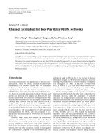
MSE
×10
−4
2
1
0
10 15 20 25 30
N
Figure 3: Mean square error (MSE) of

θ
D
as a function of number
of observations N.
Figure 3 shows the MSE of

θ
D
as a function of the num-
ber of timing messages N. It is evident that the MLE performs
well even for small N and hence suitable for the power lim-
ited regime of WSNs.
4. CONCLUSIONS AND FUTURE WORK
Using a quadratic model for the relationship between the
clocks of two nodes with a two-way timing message exchange
mechanism, we have derived the MLE for the clock offset,
skew, drift, and the fixed delay between the two nodes. In
addition, complete steps for the algorithm required to find
this MLE are also presented. Using the better model results

in long-term synchronization between nodes and conse-
quently saves a lot of energy in terms of considerably less fre-
quent resynchronization through timing message commu-
nications. For future work, deriving the Cramer-Rao lower
bound (CRLB) for the clock parameters derived in this pa-
per is a very challenging open research problem.
REFERENCES
[1] D. Mills, “Internet time synchronization: the network time
protocol,” Working Group Report RFC 1129, University of
Delaware, Newark, Del, USA, October 1989, Internet Request
for Comments.
[2] S. Ganeriwal, R. Kumar, and M. B. Srivastava, “Timing-sync
protocol for sensor networks,” in Proceedings of the 1st Interna-
tional Conference on Embedded Networked Sens or Systems (Sen-
Sys ’03), pp. 138–149, ACM Press, Los Angeles, Calif, USA,
November 2003.
[3] J. Elson, L. Girod, and D. Estrin, “Fine-grained network time
synchronization using reference broadcasts,” in Proceedings of
the 5th Symposium on Operating Systems Design and Imple-
mentation (OSDI ’02), vol. 36, pp. 147–163, Boston, Mass,
USA, December 2002.
[4] M. Mar
´
oti,B.Kusy,G.Simon,and
´
A. L
´
edeczi, “The flood-
ing time synchronization protocol,” in Proceedings of the 2nd
International Conference on Embedded Networked Sensor Sys-

tems (SenSys ’04), pp. 39–49, ACM Press, Baltimore, Md, USA,
November 2004.
[5]G.Simon,M.Mar
´
oti,
´
A. L
´
edeczi, et al., “Sensor network-
based counter sniper system,” in Proceedings of the 2nd Interna-
tional Conference on Embedded Networked Sens or Systems (Sen-
Sys ’04), pp. 1–12, Baltimore, Md, USA, November 2004.
[6] CENS habitat sensig group at James Reserve, http://www
.jamesreserve.edu/.
[7] H. S. Abdel-Ghaffar, “Analysis of synchronization algorithms
with time-out control over networks with exponentially sym-
metric delays,” IEEE Transactions on Communications, vol. 50,
no. 10, pp. 1652–1661, 2002.
[8] D. R. Jeske, “On maximum-likelihood estimation of clock off-
set,” IEEE Transactions on Communications,vol.53,no.1,pp.
53–54, 2005.
[9] S. M. Kay, Fundamentals of Statistical Signal Processing, Volume
I: Estimation Theory, Prentice-Hall, Upper Saddle River, NJ,
USA, 1993.
[10] C. Bovy, H. Mertodimedjo, G. Hooghiemstra, H. Uijterwaal,
and P. Mieghem, “Analysis of end-to-end delay measurements
in internet,” in Proceedings of the Passive and Active Measure-
ment (PAM ’02), pp. 26–33, Fort Collins, Colo, USA, March
2002.
[11] A. Papoulis, Probability, Random Variables, and Stochastic Pro-

cesses, McGraw-Hill, New York, NY, USA, 3rd edition, 1991.
[12] L. Leon-Garcia, Probability and Random Processes for Electrical
Engineering, Addison-Wesley, Reading, Mass, USA, 2nd edi-
tion, 1993.
[13] S. Moon, P. Skelly, and D. Towsley, “Estimation and removal of
clock skew from network delay measurements,” in Proceedings
of the 18th Annual Joint Conference of the IEEE Computer and
Communications Societie (INFOCOM ’99), pp. 227–234, New
York, NY, USA, March 1999.
[14] V. Paxson, “On calibrating measurements of packet transit
times,” in Proceedings of the ACM SIGMETRICS Joint Interna-
tional Conference on Measurement and Modeling of Computer
Systems, pp. 11–21, Madison, Wis, USA, June 1998.
[15] G. J. Pottie and W. J. Kaiser, “Wireless integrated network sen-
sors,” Communications of the ACM, vol. 43, no. 5, pp. 51–58,
2000.