Báo cáo hóa học: " Research Article Diversity Analysis of Distributed Space-Time Codes in Relay Networks with Multiple Transmit/Receive Antennas" pot
Bạn đang xem bản rút gọn của tài liệu. Xem và tải ngay bản đầy đủ của tài liệu tại đây (904.22 KB, 17 trang )
Hindawi Publishing Corporation
EURASIP Journal on Advances in Signal Processing
Volume 2008, Article ID 254573, 17 pages
doi:10.1155/2008/254573
Research Article
Diversity Analysis of Distributed Space-Time Codes in Relay
Networks with Multiple Transmit/Receive Antennas
Yindi Jing
1
and Babak Hassibi
2
1
Department of Electrical Engineering and Computer Science, University of California, Irvine, CA 92697, USA
2
Department of Electrical Engineering, California Institute of Technology, Pasadena, CA 91125, USA
Correspondence should be addressed to Yindi Jing,
Received 1 May 2007; Revised 13 September 2007; Accepted 28 November 2007
Recommended by M. Chakraborty
The idea of space-time coding devised for multiple-antenna systems is applied to the problem of communication over a wireless
relay network, a strategy called distributed space-time coding, to achieve the cooperative diversity provided by antennas of the relay
nodes. In this paper, we extend the idea of distributed space-time coding to wireless relay networks with multiple-antenna nodes
and fading channels. We show that for a wireless relay network with M antennas at the transmit node, N antennas at the receive
node, and a total of R antennas at all the relay nodes, provided that the coherence interval is long enough, the high SNR pairwise
error probability (PEP) behaves as (1/P)
min {M,N}R
if M
/
=N and (log
1/M
P/P)
MR
if M = N,whereP is the total power consumed
by the network. Therefore, for the case of M
/
=N, distributed space-time coding achieves the maximal diversity. For the case of
M
= N, the penalty is a factor of log
1/M
P which, compared to P, becomes negligible when P is very high.
Copyright © 2008 Y. Jing and B. Hassibi. This is an open access article distributed under the Creative Commons Attribution
License, which permits unrestricted use, distribution, and reproduction in any medium, provided the original work is properly
cited.
1. INTRODUCTION
It is known that multiple antennas can greatly increase the
capacity and reliability of a wireless communication link in a
fading environment using space-time coding [1–4]. Recently,
with the increasing interestin ad hoc networks, researchers
have been looking for methods to exploit spatial diversity
using the antennas of different users in the network [5–
24]. Many cooperative strategies are proposed, for example,
amplify-and-forward (AF) [11, 13, 14, 16, 21, 23], decode-
and-forward (DF) [9, 10, 14, 16, 22], and coded cooperation
[15]. In [7], the authors proposed the use of space-time codes
based on Hurwitz-Radon matrices in wireless relay networks.
This work follows the strategy of [5], where the idea
of space-time coding devised for multiple-antennasystems
is applied to the problem of communication over a wire-
less relay network. (Though having the same name, the
distributed space-time coding idea in [5]isdifferent from
that in [14]. Similar ideas for networks with one and two
relays have appeared in [6, 11].) In [5], the authors consider
wireless relay networks in which every node has a single
antenna and the channels are fading, and use a cooperative
strategy called distributed space-time coding by applying a
linear dispersion space-time code [25] among the relays.
It is proved that without any channel knowledge at the
relays, a diversity of R(1
− log log P/ logP) can be achieved,
where R is the number of relays and P is the total power
consumed in the whole network. This result is based on the
assumption that the receiver has full knowledge of the fading
channels. Therefore, when the total transmit power P is high
enough, the wireless relay network achieves the diversity of
a multiple-antenna system with R transmit antennas and
one receive antenna, asymptotically. That is, antennas of the
relays work as antennas of the transmitter although they
cannot fully cooperate and do not have full knowledge of the
transmit signal. After the appearance of [5], code designs for
distributed space-time coding have been proposed in [26–
31] and the differential use of distributed space-time coding
has been introduced in [32–35]. The references [36, 37]ana-
lyze the diversity-multiplexing tradeoff of distributed space-
time coding. Distributed space-time coding in asynchronous
networks is discussed in [38–43]. Other related papers can be
found in [44–46].
This paper has two main contributions. First, we extend
the idea of distributed space-time coding to wireless relay
networks whose nodes have multiple antennas. Second and
2 EURASIP Journal on Advances in Signal Processing
more importantly, based on the pairwise error probability
(PEP) analysis, we prove lower bounds on the diversity of
this scheme. We use the same two-step transmission method
in [5], where in one step the transmitter sends signals to
the relays and in the other the relays encode their received
signals into a linear dispersion space-time code and transmit
to the receiver. For a wireless relay network with M antennas
at the transmitter, N antennas at the receiver, and a total
of R antennas at all the relay nodes, our work shows that
when the coherence interval is long enough, a diversity of
min
{M, N}R if M
/
=N and MR(1−(1/M)(log log P/ log P))
if M
= N can be achieved, where P is the total power used in
the network. With this two-step protocol, it is easy to see that
the errorprobability is determined by the worse of the two
steps: the transmission from the transmitter to the relays and
the transmission from the relays to the receiver. Therefore,
when M
/
=N, distributed space-time coding is optimal since
the diversity of the first stage cannot be larger than MR,
the diversity of a multiple-antenna system with M transmit
antennas and R receive antennas, and the diversity of the
second stage cannot be larger than NR. When M
= N,
the penalty on the diversity, because the relays cannot fully
cooperate and do not have full knowledge of the signal,
is R(log logP/ logP). When P isveryhigh,itisnegligible.
Therefore, with distributed space-time coding, wireless relay
networks achieve the same diversity of multiple-antenna
systems, asymptotically.
The paper is organized as follows. In the following
section, the network model and the generalized distributed
space-time coding are explained in detail. A training scheme
is also proposed. The PEP is first analyzed in Section 3.
In Section 4, the diversity for the network with an infinite
number of relays is discussed. Then, the diversity for the
general case is obtained in Section 5. Section 6 contains
the conclusion. Proofs of some of the technical theorems
are given in Appendices A–D.InAppendix E, we discuss
heterogeneous networks.
2. WIRELESS RELAY NETWORK
2.1. Network model and distributed space-time coding
We first introduce some notation. For a complex matrix A,
A, A
t
,andA
∗
denote the conjugate, the transpose, and the
Hermitian of A,respectively.detA,rankA,andtrA indicate
the determinant, rank, and trace of A,respectively.
A denotes
the vectorization of A formed by stacking the columns of X
into a single column vector. I
n
denotes the n × n identity
matrix and 0
m,n
is the m × n matrix with all zero entries.
We often omit the subscripts when there is no confusion. log
indicates the natural logarithm.
·indicates the Frobenius
norm. P and E indicate the probability and the expected
value. g(x)
= O( f (x)) means that lim
x→∞
(g(x)/f(x)) is a
constant. h(x)
= o( f (x)) means that lim
x→∞
(h(x)/f(x)) =
0. a is the minimal integer that is not less than a.
Consider a wireless network with R +2nodeswhich
are placed randomly and independently according to some
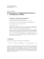
distribution. As shown in Figure 1, there are one transmit
node and one receive node. All the other R nodes work
Tr an smi t te r Re ce iv er
Relays
f
11
f
1R
f
M1
f
MR
g
11
g
1N
.
.
.
.
.
.
.
.
.
.
.
.
.
.
.
r
1
t
1
r
R
t
R
g
R1
g
RN
Step 1: time 1 to T Step 2: time T +1to2T
Figure 1: Wireless relay network with multiple-antenna nodes.
as relays. The transmitter has M transmit antennas, the
receiver has N receive antennas, and the ith relay has R
i
antennas. Since the transmit and received signals at different
antennas of the same relay can be processed and designed
independently, the network can be transformed to a network
with R
=
R
i=1
R
i
single-antenna relays by designing the
transmit signal at every antenna of every relay according to
the received signal at that antenna only. This is one possible
scheme. In general, the signal sent by one antenna of a relay
can be designed using received signals at all antennas of the
relay. However, as will be seen later, this simpler scheme
achieves the optimal diversity asymptotically although a
general design may improve the coding gain of the network.
Therefore, to highlight the diversity results by simplifying
notation and formulas, in the following, we assume that
every relay has a single antenna. Denote the channel vector
from the M antennas of the transmitter to the ith relay as
f
i
= [
f
1i
··· f
Mi
]
t
, and the channels from the ith relay
to the N antennas at the receiver as g
i
= [
g
i1
··· g
iN
].
We use the block-fading model [2]byassumingacoherence
interval T. From the two-step protocol that will be discussed
in the following, we can see that we only need f
i
to keep
constant for the first step of the transmission and g
i
to keep
constant for the second step. It is thus good enough to choose
T as the minimum of the coherence intervals of f
i
and g
i
.
Also, perfect symbol-level synchronization is assumed in this
network model. For asynchronized networks, please refer to
[38–43].
The information bits are encoded into T
× M matrices
s
, whose mth column is the signal sent by the mth transmit
antenna. For the power analysis, s
is normalized as
Etrs
∗
s = M. (1)
To s e n d s
to the receiver, the same two-step strategy in [5]is
used, as shown in Figure 1. In step one, the transmitter sends
P
1
T/Ms. The average total power used at the transmitter for
the T transmissions is P
1
T. The received signal vector and the
noise vector at the ith relay are denoted as r
i
and v
i
.Instep
two, the ith relay sends t
i
. The received signal and noise at the
receiver are denoted as X and w
. The noises are assumed to
be i.i.d. CN (0, 1). Clearly,
r
i
=
P
1
T/Msf
i
+ v
i
,
X
=
t
1
··· t
R
G + w,
(2)
where G
= [
g
t
1
··· g
t
R
]
t
.
Y. Jing and B. Hassibi 3
We use distributed space-time coding proposed in [5]by
designing the transmit signal at relay i as a linear function of
its received signal:
t
i
=
P
2
P
1
+1
A
i
r
i
,(3)
where A
i
is a predetermined T × T unitary matrix known to
both the ith relay and the receiver. It is fixed during training
and data transmissions. For various methods on how to
design the A
i
,see[26–31]. P
2
can be proved to be the average
transmit power for one transmission at every relay. After
some calculation, the system equation can be written as
X
=
P
1
P
2
T
M
P
1
+1
SH + W,(4)
where
S
=
A
1
s ··· A
R
s
, H =
f
1
g
1
t
···
f
R
g
R
t
t
,
(5)
W
=
P
2
P
1
+1
⎡
⎣
R
i=1
g
i1
A
i
v
i
···
R
i=1
g
iN
A
i
v
i
⎤
⎦
+ w. (6)
The received signal matrix, X,isT
×N. S,whichisT ×MR,
is the linear distributed space-time code. Since f
i
is M ×1and
g
i
is 1 × N, the equivalent channel matrix H is RM × N. W,
which is T
×N, is the equivalent noise matrix.
Define
R
W
= I +
P
2
1+P
1
G
∗
G. (7)
The covariance matrix of the equivalent noise matrix can
be proved to be
R
W
. The diversity analysis in this paper is
much more difficult than that in [5] because in networks
with single-antenna nodes, the covariance matrix of the
equivalent noise is a multiple of the identity matrix. Here,
for the diversity result, we need to analyze the eigenvalues of
R
W
or find bounds on them.
2.2. Assumptions and training
In this paper, we assume that f
mi
and g
in
have independent
Rayleigh distributions; that is, f
mi
and g
in
are independent
circulant complex Gaussian random variables with zero
mean. For simplicity, we also assume that f
mi
and g
in
have
the same variance, which is 1. The heterogeneous case, in
which every channel has a different variance, is discussed in
Appendix E. The same diversity results can be obtained in
heterogeneous networks. We make the practical assumption
that the relays have no channel information. However, we do
assume that the receiver has enough channel information to
do coherent detection. Thus, a training process is needed.
For coherence ML decoding at the receiver, the receiver
needs to know H and
R
W
,orequivalently,H and G.We
propose a training process that contains two steps and takes
M
p
+2N
p
symbol periods (other training methods can also
be envisioned, and the one proposed here is one possibility).
Each step mimics the training process of a multiple-antenna
system [47] as its system equation has the same structure.
First, we estimate G, which takes M
p
symbol periods. Let
U
p
be a predesigned full-rank M
p
× R pilot matrix. The ith
relay sends the ith column of U
p
simultaneously. The receiver
gets
Y
p
=
Q
p
M
p
R
U
p
G + w
p
,(8)
where Q
p
is the power used at every relay and w
p
is
the M
p
× N noise matrix. Since there are RN unknowns
(corresponding to the components of G)andmin
{M
p
, R}N
independent equations, we need M
p
≥ R.Wecouldestimate
G from U
p
using ML, MMSE, or other criteria.
Then, we estimate H using distributed space-time coding
discussed in Section 2.1. This takes 2N
p
symbol periods. The
transmitter sends a full-rank N
p
× M pilot signal matrix s
p
and the relays perform distributed space-time coding. From
(4), the received signal can be written as
X
p
=
P
1,p
P
2,p
N
p
M(P
1,p
+1)
S
p
H + W
p
,(9)
where P
1,p
and P
2,p
are the powers used at the transmitter
and every relay and
S
p
=
A
1
s
p
··· A
R
s
p
(10)
is the carefully designed N
p
×MR pilot space-time codeword.
Now, let us discuss the number of training symbols needed
in this step. Note that G is known from the first training step.
Define
f
=
f
t
1
··· f
t
R
t
. (11)
By stacking the columns of X into one single column vector,
we can rewrite (9)as
X
p
=
P
1,p
P
2,p
N
p
M
P
1,p
+1
⎡
⎢
⎢
⎢
⎢
⎣
S
p
diag
g
11
I
M
, , g
R1
I
M
.
.
.
S
p
diag
g
1N
I
M
, , g
RN
I
M
⎤
⎥
⎥
⎥
⎥
⎦
f +
W
p
=
P
1,p
P
2,p
N
p
M
P
1,p
+1
⎡
⎢
⎢
⎢
⎢
⎣
g
11
A
1
s
p
··· g
R1
A
R
s
p
.
.
.
.
.
.
.
.
.
g
1N
A
1
s
p
··· g
RN
A
R
s
p
⎤
⎥
⎥
⎥
⎥
⎦
f +
W
p
=
P
1,p
P
2,p
N
p
M
P
1,p
+1
⎡
⎢
⎢
⎢
⎢
⎣
g
11
I
N
p
··· g
R1
I
N
p
.
.
.
.
.
.
.
.
.
g
1N
I
N
p
··· g
RN
I
N
p
⎤
⎥
⎥
⎥
⎥
⎦
×
diag
A
1
s
p
, , A
R
s
p
f +
W
p
.
(12)
4 EURASIP Journal on Advances in Signal Processing
Denote
H
p
=
⎡
⎢
⎢
⎣
g
11
I
N
p
··· g
R1
I
N
p
.
.
.
.
.
.
.
.
.
g
1N
I
N
p
··· g
RN
I
N
p
⎤
⎥
⎥
⎦
diag
A
1
s
p
, , A
R
s
p
.
(13)
The number of independent equations in (9) equals the rank
of H
p
, which is min{N
p
N, N
p
R, MR}. Since there are MR
unknowns (corresponding to the components of f), we need
min
{N
p
N, N
p
R, MR}≥MR, which is equivalent to
N
p
≥ max
MR/N, M
. (14)
While this condition is satisfied, we could estimate f from
X
p
using ML, MMSE, or other criteria. The overall training
process takes at least R+2max
{MR/N, M} symbol periods.
The optimal designs of U
p
, Q
p
, S
p
(or s
p
), and P
1,p
, P
2,p
are
interesting issues. However, they are beyond the scope of this
paper.
3. PAIRWISE ERROR PROBABILITY AND
OPTIMAL POWER ALLOCATION
To analyze the PEP, we have to determine the maximum-
likelihood (ML) decoding rule. This requires the conditional
probability density function (PDF) P(X
| s
k
), where s
k
∈ S
and S is the set of all possible transmit signal matrices.
Theorem 1. Given that s
k
is transmitted, define
S
k
=
A
1
s
k
A
2
s
k
··· A
R
s
k
. (15)
Then conditioned on s
k
,therowsofX are independently
Gaussian distributed with the same variance
R
W
.Thetth row
of X has mean
P
1
P
2
T/M(P
1
+1)[S
k
]
t
H with [S
k
]
t
being the
tth row of S
k
.Also,
P
X | s
k
=
π
N
det R
W
−T
×e
−tr(X−
P
1
P
2
T/M
P
1
+1
S
k
H)R
−1
W
(X−
P
1
P
2
T/M
P
1
+1
S
k
H)
∗
.
(16)
Proof. See Appendix A.
In view of Theorem 1, we should emphasize that for a
wireless relay network with multiple antennas at the receiver,
the columns of X are not independent although the rows of
X are. (The covariance matrix of each row R
W
is not diagonal
in general.) That is, the received signals at different antennas
are not independent, whereas the received signals at different
times are. This is the main reason that the PEP analysis in the
new model is much more difficult than that of the network
in [5], where X had only a single column.
With P(X
| s
k
) in hand, we can obtain the ML decoding
and thereby analyze the PEP. The result follows.
Theorem 2 (ML decoding and the PEP Chernoff bound).
TheMLdecodingoftherelaynetworkis
arg min
s
k
tr
X −
P
1
P
2
T
M
P
1
+1
S
k
H
×
R
−1
W
X −
P
1
P
2
T
M
P
1
+1
S
k
H
∗
.
(17)
With this decoding, the PEP of mistaking s
k
by s
l
, averaged over
the channel realization, has the following upper bound:
P
s
k
−→ s
l
≤
E
f
mi
,g
in
e
−(P
1
P
2
T/4M(1+P
1
)) tr (S
k
−S
l
)
∗
(S
k
−S
l
)HR
−1
W
H
∗
.
(18)
Proof. The proof is omitted since it is the same as the proof
of Theorem 1 in [5].
As both H and R
W
are known at the receiver, sphere
decoding can be used to perform the ML decoding in (17).
The main purpose of this work is to analyze how the PEP
decays with the total transmit power. The total power used in
the whole network is P
= P
1
+ RP
2
. One natural question is
how to allocate power between the transmitter and the relays
if P is fixed. Notice that when R
→∞, according to the law
of large numbers, the off-diagonal entries of (1/R)G
∗
G go to
zero while the diagonal entries approach 1 with probability
1. It is thus reasonable to assume (1/R)G
∗
G ≈ I
N
for large
R. With this approximation, minimizing the PEP is now
equivalent to maximizing P
1
P
2
T/4M(1 + P
1
+ RP
2
). This is
exactly the same power allocation problem in [5]. Therefore,
we can conclude that the optimum solution is to set
P
1
=
P
2
, P
2
=
P
2R
.
(19)
That is, the optimum power allocation is such that the
transmitter uses half the total power and the relays share
the other half. As discussed in Section 2.1, for the general
network where the ith relay has R
i
antennas, the antennas
are treated as R
i
different relays. Therefore, in general, the
optimum power allocation is such that the transmitter uses
half the total power as before, but every relay uses a power
that is proportional to its number of antennas, that is, P
1
=
P/2 and the power used at the ith relay is R
i
P/2R.
4. DIVERSITY ANALYSIS FOR R
→∞
4.1. Basic results
As mentioned earlier, to obtain the diversity, we have to
compute the expectations over f
mi
and g
in
in (18). We will do
this rigorously in Section 5. However, since the calculation
is detailed and gives little insight, in this section, we give a
simple asymptotic derivation for the case where the number
of relay nodes approaches infinity, that is, R
→∞.As
discussed in the previous section, when R is large, we can
make the approximation R
W
≈ (1 + P
2
R/(P
1
+1))I
N
.Denote
the nth column of H as h
n
.From(5), h
n
= G
n
f,wherewe
Y. Jing and B. Hassibi 5
have defined G
n
= diag{g
1n
I
M
, , g
Rn
I
M
}. Therefore, from
(18) and using the optimal power allocation in (19),
P
s
k
−→ s
l
E
f
mi
,g
in
e
−(PT/16MR)trH
∗
(S
k
−S
l
)
∗
(S
k
−S
l
)H
= E
f
mi
,g
in
e
−(PT/16MR)
N
n
=1
h
∗
n
S
k
−S
l
∗
(S
k
−S
l
)h
n
= E
f
mi
,g
in
e
−(PT/16MR)f
∗
[
N
n
=1
G
∗
n
S
k
−S
l
∗
(S
k
−S
l
)G
n
]f
.
(20)
Since f is white Gaussian with mean zero and variance I
RM
,
P(s
k
−→ s
l
)
E
g
in
det
−1
⎡
⎣
I
RM
+
PT
16MR
N
n=1
G
∗
n
(S
k
−S
l
)
∗
(S
k
−S
l
)G
n
⎤
⎦
.
(21)
Similar to the multiple-antenna case [4, 48] and the case
of wireless relay networks with single-antenna nodes [5], to
achieve full diversity, S
k
− S
l
must be full rank. Since the
distributed space-time codes S
k
and S
l
are T × MR, in the
following, we will assume T
≥ MR and the code is fully
diverse.
Denote the minimum singular value of (S
k
−S
l
)
∗
(S
k
−
S
l
)byσ
2
min
. From the full diversity of the code, σ
2
min
>
0. Therefore, the right side of (21) can be further upper
bounded as
P
s
k
−→ s
l
E
g
in
det
−1
⎡
⎣
I
RM
+
PTσ
2
min
16MR
N
n=1
G
∗
n
G
n
⎤
⎦
=
E
g
in
R
i=1
⎛
⎝
1+
PTσ
2
min
16MR
N
n=1
g
in
2
⎞
⎠
−M
.
(22)
Since g
in
are i.i.d. CN (0,1),
N
n
=1
|g
in
|
2
are i.i.d. gamma
distributed with PDF (1/(N
−1)!)g
N−1
i
e
−g
i
. Therefore,
P
s
k
−→ s
l
1
(N − 1)!
R
⎡
⎣
∞
0
1+
PTσ
2
min
16MR
x
−M
x
N−1
e
−x
dx
⎤
⎦
R
.
(23)
By defining y
= 1+(PTσ
2
min
/16MR)x,wehave
P
s
k
−→ s
l
1
(N −1)!
R
16MR
PTσ
2
min
NR
e
16MR
2
/PTσ
2
min
×
∞
1
(y − 1)
N−1
y
M
e
−(16MR/PTσ
2
min
)y
dy
R
1
(N − 1)!
R
16MR
PTσ
2
min
NR
×
⎡
⎣
N−1
l=0
N −1
l
∞
1
y
l−M
e
−(16MR/PTσ
2
min
)y
dy
⎤
⎦
R
.
(24)
The following theorem can be obtained by calculating the
integral.
Theorem 3 (diversity for R
→∞). Assume that R →∞,
T
≥ MR, and the distributed space-time code is full diverse.
For large total transmit power P,bylookingatonlythehighest-
order term of P,thePEPofmistakings
k
by s
l
has the following
upper bound:
P
s
k
−→ s
l
1
(N − 1)!
R
16MR
Tσ
2
min
min{M,N}R
×
⎧
⎪
⎪
⎪
⎪
⎪
⎪
⎪
⎪
⎪
⎪
⎨
⎪
⎪
⎪
⎪
⎪
⎪
⎪
⎪
⎪
⎪
⎩
2
N−1
M − N
R
P
−NR
if M>N,
log
1/M
P
P
MR
if M = N,
(N
−M − 1)!
R
P
−MR
if M<N.
(25)
Therefore, the diversity of the wireless relay network is
d
=
⎧
⎪
⎪
⎪
⎪
⎨
⎪
⎪
⎪
⎪
⎩
min{M, N}R if M
/
=N,
MR
1 −
1
M
log log P
log P
if M = N.
(26)
Proof. See Appendix B.
4.2. Discussion
With the two-step protocol, it is easy to see that regardless
of the cooperative strategy used at the relay nodes, the
error probability is determined by the worse of the two
transmission stages: the transmission from the transmitter to
the relays and the transmission from the relays to the receiver.
The PEP of the first stage cannot be better than the PEP of
a multiple-antenna system with M transmit antennas and R
receive antennas, whose optimal diversity is MR, while the
PEP of the second stage can have diversity not larger than
NR. Therefore, when M
/
=N, according to the decay rate
of the PEP, distributed space-time coding is optimal. For
the case of M
= N, the penalty on the decay rate is just
R(log logP/ logP), which is negligible when P is high.
If we can use the diversity definition in [49], since
lim
P→∞
(log logP/ logP) = 0, diversity min{M, N}R can be
obtained.
The results in Theorem 6 are obtained by considering
only the highest-order term of P in the PEP formula. In brief,
we call the rth highest-order term of P in the PEP formula
6 EURASIP Journal on Advances in Signal Processing
the rth term. When analyzing the diversity, not only is the
first term important, but also how dominant it is. Therefore,
we should analyze the contributions of the second and also
other terms of P compared to those of the first one. This is
equivalent to analyzing how large the total transmit power P
should be for the terms in (25) to dominate. The following
remarks are on this issue. They can be observed from the
proof of Theorem 3 in Appendix B.
Remark 1. (1) If
|M − N| > 1, from (B.13)and(B.22),
the second term behaves as P
−min{M,N}R+1
.Thedifference
between the first and second terms is a P factor. Therefore,
the first term is dominant when P
1. In other words,
contributions of the second and other terms are negligible
when P
1.
(2) If M
= N,from(B.16), the second term is
2
M−1
R
(M − 1)!
R
16MR
Tσ
2
min
MR
log
R−1
P
P
MR
, (27)
which has one less logP than the first one. Therefore, the
first term, (1/(M
− 1)!
R
)(16MR/Tσ
2
min
)
MR
(log
1/M
P/P)
MR
,is
dominant if and only if log P
1, which is a much
stronger condition than P
1. When P is not very large,
contributions of the second and even other terms are not
negligible.
(3) If
|M − N|=1, from (B.11)and(B.24), the
second term behaves as P
−min{M,N}R
(log P/P). The difference
between the first and second terms is log P/P factor. There-
fore, the first term given in (25) is dominant if and only
if P
log P. This condition is weaker than the condition
log P
1 in the previous case; however, it is still stronger
than the normally used condition P
1.
5. DIVERSITY ANALYSIS FOR THE GENERAL C ASE
5.1. A simple derivation
The diversity analysis in the previous section is based on the
assumption that the number of relays is very large. In this
section, analysis on the PEP and diversity for networks with
any number of relays is given.
As discussed in Section 3, the main difficulty of the PEP
analysis lies in the fact that the noise covariance matrix R
W
is not diagonal. From (18), we can see that one way of upper
bounding the PEP is to upper bound R
W
. Since R
W
≥ 0,
R
W
≤
tr R
W
I
N
=
⎛
⎝
N +
P
2
P
1
+1
N
n=1
R
i=1
g
in
2
⎞
⎠
I
N
. (28)
Therefore, from (18) and using the power allocation given in
(19),
P
s
k
−→ s
l
E
f
mi
,g
in
e
−(PT/8MNR(1+(1/NR)
N
n
=1
R
i
=1
g
in
2
))tr H
∗
(S
k
−S
l
)
∗
(S
k
−S
l
)H
(29)
when P
1. If the space-time code is fully diverse, using
similar argument in the previous section,
P
s
k
−→ s
l
E
g
in
R
i=1
1+
PTσ
2
min
8MNR
g
i
1+(1/NR)
R
i=1
g
i
−M
,
(30)
where, as before, σ
2
min
is the minimum singular value of
(S
k
−S
l
)
∗
(S
k
− S
l
)andg
i
=
N
n=1
|g
in
|
2
. Calculating this
integral, the following theorem can be obtained.
Theorem 4 (diversity for wireless relay network). Assume
that T
≥ MR andthedistributedspace-timecodeisfulldiverse.
For large total transmit power P, by looking at the highest-order
terms of P,thePEPofmistakings
k
by s
l
satisfies
P(s
k
−→ s
l
)
1
(N −1)!
R
8MNR
Tσ
2
min
min{M,N}R
×
⎧
⎪
⎪
⎪
⎪
⎪
⎪
⎪
⎪
⎪
⎪
⎪
⎪
⎨
⎪
⎪
⎪
⎪
⎪
⎪
⎪
⎪
⎪
⎪
⎪
⎪
⎩
M
N(M − N)
R
P
−NR
if M>N,
1+
1
N
R
log
1/M
P
P
MR
if M = N,
1
N
+(N
−M − 1)!
R
P
−MR
if M<N.
(31)
Therefore,thesamediversityasin(26) is obtained.
Proof. See Appendix C.
Although the same diversity is obtained as in the R →
∞
case, there is a factor of N in (31), which does not
appear in (25). This is because we upper bound R
W
by
(trR
W
)I
N
, whose expectation is N times the expectation
of R
W
, while in the previous subsection we approximate
R
W
by its expectation. This factor of N can be avoided by
tighter upper bounds of R
W
.Inthefollowingsubsection,we
analyze the maximum eigenvalue of R
W
. Then in Section 5.3,
a PEP upper bound using the maximum eigenvalue of R
W
is
obtained.
5.2. The maximum eigenvalue of Wishart matrix
Denote the maximum eigenvalue of (1/R)G
∗
G as λ
max
. Since
G is a random matrix, λ
max
is a random variable. We first
analyze the PDF and the cumulative distribution function
(CDF) of λ
max
.
If entries of G are independent Gaussian distributed with
mean zero and variance one, or equivalently, both the real
and imaginary parts of every entry in G are Gaussian with
mean zero and variance 1/2, (1/R)G
∗
G is known as the
Wishart matrix. While there exists explicit formula for the
distribution of the minimum eigenvalue of a Wishart matrix,
we could not find nonasymptotic formula for the maximum
eigenvalue. Therefore, we calculate the PDF and CDF of λ
max
from the joint distribution of all the eigenvalues of (1/R)G
∗
G
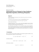
in this section. The following theorem has been proved.
Y. Jing and B. Hassibi 7
0
0.5
1
1.5
2
2.5
3
Pr (λ
max
= λ)
01
2345
λ
R
= 10 N = 2
R
= 10 N = 3
R
= 10 N = 4
R
= 40 N = 2
R
= 40 N = 3
R
= 40 N = 4
PDF of λ
max
of Wishart matrix
Figure 2: PDF of the maximum eigenvalue of (1/R)G
∗
G.
Theorem 5. Assume that R ≥ N and G is an R × N matrix
whose entries are i.i.d. CN (0,1).
(1) The PDF of the maximum eigenvalue of (1/R)G
∗
G is
p
λ
max
(λ) =
R
RN
λ
R−N
e
−Rλ
N
n=1
Γ(R − n +1)Γ(n)
det F, (32)
where F is an (N
− 1) × (N − 1) Hankel matrix whose
(i, j)th entry equals f
ij
=
λ
0
(λ − t)
2
t
R−N+i+ j−2
e
−Rt
dt.
(2) The CDF of the maximum eigenvalue of (1/R)G
∗
G is
P
λ
max
≤ λ
=
R
RN
N
n
=1
Γ(R − n +1)Γ(n)
det F
, (33)
where F
is an N ×N Hankel matrix whose (i, j)th entry
equals f
ij
=
λ
0
t
R−N+i+ j−2
e
−Rt
dt.
Proof. See Appendix D.
A theoretical analysis of the PDF and CDF from (32)
and (33)appearstobequitedifficult. To understand λ
max
,
we plot the two functions in Figures 2 and 3 for different R
and N. Figure 2 shows that the PDF has a peak at a value a
bit larger than 1. As R increases, the peak becomes sharper.
An increase in N shifts the peak right. However, the effect is
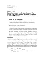
smaller for larger R.FromFigure 3, the CDF of λ
max
grows
rapidly around λ
= 1andbecomesverycloseto1soonafter.
The larger R is, the faster the CDF grows. Similar to the PDF,
an increase in N results in a right shift of the CDF. However,
as R grows, the effect diminishes. This verifies the validity of
the approximation G
∗
G ≈ RI
N
in Section 4 for large R.
In the following corollary, we give an upper bound on
the PDF. This result is used to derive the diversity result for
general R in the next subsection.
0
0.2
0.4
0.6
0.8
1
Pr (λ
max
<λ)
01
2345
λ
R
= 10 N = 2
R
= 10 N = 3
R
= 10 N = 4
R
= 40 N = 2
R
= 40 N = 3
R
= 40 N = 4
CDF of λ
max
of Wishart matrix
Figure 3: CDF of the maximum eigenvalue of (1/R)G
∗
G.
Corollary 1. When R ≥ N, the PDF of the maximum
eigenvalue of (1/R)G
∗
G can be upper bounded as
p
λ
max
(λ) ≤ C
1
λ
RN−1
e
−Rλ
, (34)
where
C
1
=
1
N
n
=1
Γ(R − n +1)Γ(n)
×
2
N−1
R
RN
N−1
n=1
(R − N +2n − 1)(R −N +2n)(R − N +2n +1)
(35)
is a constant that depends only on R and N.
Proof. From the proof of Theorem 5, F is a positive semidef-
inite matrix. Therefore, det F
≤
N−1
n
=1
f
nn
.From(32), f
nn
can
be upper bounded as
f
nn
≤
λ
0
(λ − t)
2
t
R−N+2n−2
dt
=
2
(R − N +2n − 1)(R −N +2n)(R − N +2n +1)
×λ
R−N+2n+1
,
(36)
then we have
det F
≤
2
N−1
N−1
n
=1
(R − N +2n − 1)(R −N +2n)(R − N +2n +1)
×λ
RN−R+N−1
.
(37)
Thus, (34) is obtained.
8 EURASIP Journal on Advances in Signal Processing
5.3. Bound on PEP from bound on eigenvalues
If the maximum eigenvalue of (1/R)G
∗
G is λ
max
, the maxi-
mum eigenvalue of R
W
is 1+(P
2
R/(P
1
+1))λ
max
, and therefore
R
W
≤ (1 + (P
2
R/(P
1
+1))λ
max
)I
N
.From(20) and using the
power allocation given in (19), we have
P
s
k
−→ s
l
| λ
max
= c
≤
E
f
mr
,g
rn
e
−(P
1
P
2
T/4M(1+P
1
+P
2
Rλ
max
))tr(S
k
−S
l
)
∗
(S
k
−S
l
)HH
∗
E
f
mr
,g
rn
e
−(PT/8(1+λ
max
)MR)tr(S
k
−S
l
)
∗
(S
k
−S
l
)HH
∗
.
(38)
The only difference of the above formula with formula (20)is
that the coefficient in the constant in the denominator of the
exponent is 8(1 + λ
max
) now instead of 16. This makes sense
since c
→ 1asR →∞. Therefore, using an argument similar
to the proof of Theorem 3, at high total transmit power, by
looking at the highest-order terms of P,
P
s
k
−→ s
l
| λ
max
=c
1
(N −1)!
R
8(1+c)MR
Tσ
2
min
min{M,N}R
×
⎧
⎪
⎪
⎪
⎪
⎪
⎪
⎪
⎪
⎪
⎨
⎪
⎪
⎪
⎪
⎪
⎪
⎪
⎪
⎪
⎩
2
N−1
M − N
R
P
−NR
if M>N,
log
1/M
P
P
MR
if M = N,
(N
−M − 1)!
R
P
−MR
if M<N.
(39)
The following theorem can thus be obtained.
Theorem 6 (diversity for wireless relay network). Assume
that T
≥ MR andthedistributedspace-timecodeisfulldiverse.
For large total transmit power P, by looking at the highest-order
terms of P, the PEP of mistaking s
k
by s
l
can be upper bounded
as
P
s
k
−→ s
l
C
(N −1)!
R
8MR
Tσ
2
min
min{M,N}R
×
⎧
⎪
⎪
⎪
⎪
⎪
⎪
⎪
⎪
⎪
⎪
⎨
⎪
⎪
⎪
⎪
⎪
⎪
⎪
⎪
⎪
⎪
⎩
2
N−1
M − N
R
P
−NR
if M>N,
log
1/M
P
P
MR
if M = N,
(N
−M − 1)!
R
P
−MR
if M<N,
(40)
where
C=
⎧
⎪
⎪
⎪
⎪
⎪
⎪
⎪
⎪
⎪
⎨
⎪
⎪
⎪
⎪
⎪
⎪
⎪
⎪
⎪
⎩
C
1
min
{M,N}R
i=0
⎛
⎝
min{M, N}R
i
⎞
⎠
(RN + i −1)!
R
RN+i
if R≥N,
C
2
min
{M,N}R
i=0
⎛
⎝
min{M, N}R
i
⎞
⎠
(RN + i −1)!
R
i
N
RN
if R<N,
C
2
=
1
R
r=1
Γ(N − r +1)Γ(r)
×
2
R−1
N
RN
R−1
r=1
(N − R +2r − 1)(N −R +2r)(N −R +2r +1)
.
(41)
Therefore,thesamediversityasin(26) is obtained.
Proof. When R
≥ N,
P
s
k
−→ s
l
=
∞
0
P
s
k
−→ s
l
| λ
max
= c
p
λ
max
(c)dc
≤
∞
0
C
1
c
RN−1
e
−Rc
P
s
k
−→ s
l
| λ
max
= c
dc
(42)
using (34)inCorollary 1.From(39),
P
s
i
−→ s
i
C
1
(N − 1)!
R
8MR
Tσ
2
min
min{M,N}R
×
∞
0
c
RN−1
e
−Rc
(1 + c)
min{M,N}R
dc
×
⎧
⎪
⎪
⎪
⎪
⎪
⎪
⎪
⎪
⎪
⎪
⎨
⎪
⎪
⎪
⎪
⎪
⎪
⎪
⎪
⎪
⎪
⎩
2
N−1
M − N
R
P
−NR
if M>N,
log P
P
M
R
if M = N,
(N
−M − 1)!
R
P
−MR
if M<N.
(43)
Since
∞
0
c
RN−1
e
−Rc
(1 + c)
min{M,N}R
dc
=
min{M,N}R
i=0
min{M, N}R
i
(RN + i −1)!
R
RN+i
,
(44)
(40) is obtained.
For the case of R<N, G
∗
is an N × R (N>R)
matrix whose entries are i.i.d. CN(0, 1). Denote the maximal
eigenvalue of (1/N)GG
∗
as λ
max
. Its PDF and CDF are given
in Theorem 5 with R and N being switched. Using the facts
that the maximal eigenvalue of (1/R)G
∗
G is (N/R)λ
max
and
∞
0
c
RN−1
e
−Nc
1+
N
R
c
min{M,N}R
dc
=
min{M,N}R
i=0
min{M, N}R
i
(RN + i −1)!
R
i
N
RN
,
(45)
we can finish the proof of this theorem.
Y. Jing and B. Hassibi 9
6. SIMULATION RESULTS
In this section, we show simulated block error rates of
three networks with multiple transmit/receive antennas and
compare them with the three PEP bounds we derived in
(25), (31), and (40). These bounds are also addressed as PEP
bound 1, PEP bound 2, and PEP bound 3 for the sake of
presentation. The main purpose of this section is to verify
the diversity results in (26). The optimal code design is not
an issue. In the simulations, we use the power allocation in
(19) and the ML decoding in (17). It is known that with ML
metric, a factor of 1/2 can be applied to Chernoff bounds
on the two-signal error rate, which is the block error rate
when there are two possible transmit signals. Thus, the PEP
bounds shown in Figures 4–6 are calculated from (25), (31),
and (40) with a factor of 1/2. In all figures, the horizontal
axis indicates P, the total transmit power used in the whole
network.
Our first example, whose performance is shown in
Figure 4, is a network with one transmit antenna, two relay
antennas, and two receive antennas, that is, M
= 1, R = 2,
N
= 2. We set T = MR = 2. The transmit signal is designed
as
s
=
s
1
s
2
t
, (46)
where s
1
and s
2
are chosen as BPSK signals (normalized
according to (1)).Thematricesusedatrelaysaredesigned
as
A
1
= I
2
, A
2
=
0 −1
10
. (47)
The distributed space-time codeword formed at the receiver
S is thus a 2
× 2realorthogonaldesign[50]. Then, we show
performance of a network with M
= 2, R = 2, N = 1in
Figure 5.WesetT
= MR = 4. The transmit signal is deigned
as
s
=
⎡
⎢
⎢
⎢
⎣
s
1
−s
2
s
2
s
1
s
3
−s
4
s
4
s
3
⎤
⎥
⎥
⎥
⎦
, (48)
where s
1
, s
2
, s
3
, s
4
are also BPSK signals (normalized
according to (1)).Thematricesusedatrelaysaredesigned
as
A
1
= I
4
, A
2
=
⎡
⎢
⎢
⎢
⎣
00−10
00 0 1
10 0 0
01 0 0
⎤
⎥
⎥
⎥
⎦
. (49)
The distributed space-time codeword formed at the receiver
S is thus a 4
× 4realorthogonaldesign[50]. Finally, in
Figure 6, we show performance of a network with M
= 2,
R
= 1, N = 2. We set T = MR = 2. The transmit signal is
10
−5
10
−4
10
−3
10
−2
10
−1
10
0
Block error rate
10 12 14 16 18 20 22 24 26 28 30
P (dB)
2-signal error rate
Block error rate
PEP bound 1
PEP bound 2
PEP bound 3
Figure 4: M = 1, R = 2, N = 2, T = 2.
10
−5
10
−4
10
−3
10
−2
10
−1
10
0
Block error rate
10 12 14 16 18 20 22 24 26 28 30
P (dB)
2-signal error rate
Block error rate
PEP bound 1
PEP bound 2
PEP bound 3
Figure 5: M = 2, R = 2, N = 1, T = 4.
designed as
s
=
s
1
−s
2
s
2
s
1
, (50)
where s
1
and s
2
are BPSK signals (normalized according to
(1)). The matrices used at the relay are set to be I
2
.The
distributed space-time codeword formed at the receiver S is
again a 2
× 2realorthogonaldesign[50]. The transmission
rate of all three networks can be calculated to be 1/2. For
comparison, we also show the 2-signal error rates of the three
networks by fixing s
2
, , s
T
.
10 EURASIP Journal on Advances in Signal Processing
10
−5
10
−4
10
−3
10
−2
10
−1
10
0
Block error rate
10 12 14 16 18 20 22 24 26 28 30
P (dB)
2-signal error rate
Block error rate
PEP bound 1
PEP bound 2
PEP bound 3
Figure 6: M = 2, R = 1, N = 2, T = 2.
Figures 4–6 indicate that when the transmit power is
high, all three networks achieve the diversities shown by the
PEP bounds. This verifies our diversity result in (26). PEP
bound 1 is the tightest of the three. This is because PEP
bound 1 is obtained by approximating R
W
by its asymptotic
(R
→∞) limit, which is also its mean; however, strict lower
bounds on R
W
are used in the calculations of bound 2 and
bound 3. In Figure 5, the three bounds are very close to each
other and, actually, bounds 1 and 2 are the same.
7. CONCLUSIONS
In this paper, we generalize the idea of distributed space-time
coding to wireless relay networks whose transmitter, receiver,
and/or relays can have multiple antennas. We assume that the
channel information is only available at the receiver. The ML
decoding at the receiver and PEP of the network are analyzed.
We have shown that for a wireless relay network with M
antennas at the transmitter, N antennas at the receiver, a total
of R antennas at all the relay nodes, and a coherence interval
not less than MR, an achievable diversity is min
{M, N}R
if M
/
=N and MR(1 − (1/M)(log log P/ log P)) if M = N,
where P is the total power used in the whole network.
This result shows the optimality of distributed space-time
coding according to the diversity gain. Simulation results are
exhibited to justify our diversity analysis.
APPENDICES
A. PROOF OF THEOREM 1
Proof. It is obvious that since H is known and W is Gaussian,
the rows of X are Gaussian. We only need to show that
the rows of X are uncorrelated and that the mean and
variance of the tth row are
(P
1
P
2
T/(P
1
+1)M)[S
k
]
t
H and
R
W
,respectively.
The (t,n)th entry of X can be written as
x
tn
=
P
1
P
2
T
M(P
1
+1)
R
i=1
M
m=1
T
τ=1
f
mi
g
in
a
i,tτ
s
k,τm
+
P
2
P
1
+1
R
i=1
T
τ=1
g
in
a
i,tτ
v
iτ
+ w
tn
,
(A.1)
where a
i,tτ
is the (t, τ)th entry of A
i
and s
k,τm
is the (τ, m)th
entry of s
k
. With full channel information at the receiver,
Ex
tn
=
P
1
P
2
T
M
P
1
+1
R
i=1
M
m=1
T
τ=1
f
mi
g
in
a
i,tτ
s
k,τm
. (A.2)
Therefore, the mean of the tth row is then represented by
(P
1
P
2
T/M(P
1
+1))[S
k
]
t
H. Since v
i
, w
n
,ands
k
are inde-
pendent,
Cov
x
t
1
n
1
, x
t
2
n
2
=
E
x
t
1
n
1
−Ex
t
1
n
1
x
t
2
n
2
−Ex
t
2
n
2
=
P
2
P
1
+1
R
i
1
=1
T
τ
1
=1
R
i
2
=1
T
τ
2
=1
×Eg
i
1
n
1
a
i
1
,t
1
τ
1
v
r
1
τ
1
g
i
2
n
2
a
i
2
,t
2
τ
2
v
i
2
τ
2
+Ew
t
1
n
1
w
t
2
n
2
=
P
2
P
1
+1
R
i=1
T
τ=1
a
i,t
1
τ
a
i,t
2
τ
g
in
1
g
in
2
+ δ
n
1
n
2
δ
t
1
t
2
= δ
t
1
t
2
⎛
⎝
P
2
P
1
+1
R
r=1
g
in
1
g
in
2
+ δ
n
1
n
2
⎞
⎠
=
δ
t
1
t
2
⎛
⎜
⎜
⎜
⎜
⎝
P
2
P
1
+1
g
1n
1
··· g
Rn
1
⎛
⎜
⎜
⎜
⎜
⎝
g
1n
2
.
.
.
g
Rn
2
⎞
⎟
⎟
⎟
⎟
⎠
+ δ
n
1
n
2
⎞
⎟
⎟
⎟
⎟
⎠
.
(A.3)
The fourth equality is true since A
i
are unitary. Therefore, the
rows of X are independent since the covariance of x
t
1
n
1
and
x
t
2
n
2
is zero when t
1
/
=t
2
. It is also easy to see that the variance
matrix of each row is I
N
+(P
2
/(P
1
+1))G
t
G, which equals R
W
.
Therefore,
P
[X]
t
| s
k
=
π
N
det R
W
−T
×e
−tr[X−
√
(P
1
P
2
T/M(P
1
+1))S
k
H]
t
R
−1
W
[X−
√
(P
1
P
2
T/M(P
1
+1))S
k
H]
t
t
=
π
N
det R
W
−T
×e
−tr[X−
√
(P
1
P
2
T/M(P
1
+1))S
k
H]
t
R
−1
W
[X−
√
(P
1
P
2
T/M(P
1
+1))S
k
H]
∗
t
.
(A.4)
Since P(X
| s
k
) =
T
t
=1
P([X]
t
| s
k
), (16) can be obtained.
Y. Jing and B. Hassibi 11
B. PROOF OF THEOREM 3
Proof. Define
I
=
N−1
l=0
N −1
l
∞
1
y
l−M
e
−(16MR/PTσ
2
min
)y
dy. (B.1)
We first give three integral equalities that will be used later:
∞
u
x
n
e
−μx
dx
= e
−uμ
n
k=0
n!
k!
u
k
μ
n−k+1
, u>0, Rμ>0, n = 0, 1,2, ,
(B.2)
∞
u
e
−μx
x
n+1
dx = (−1)
n+1
μ
n
Ei(−μu)
n!
+
e
−μu
u
n
n
−1
k=0
(−1)
k
μ
k
u
k
n ···(n −k)
, μ>0, n
= 1, 2, ,
(B.3)
∞
u
e
−μx
x
dx
=−Ei(−μu), Rμ>0, u ≥ 0, (B.4)
where
Ei (χ)
=
χ
−∞
e
t
t
dt, χ<0, (B.5)
is the exponential integral function [51]. To calculate I,we
discuss the following cases separately.
Case 1 (M<N). In this case,
I
=
N−1
l=M
N −1
l
∞
1
y
l−M
e
−(16MR/PTσ
2
min
)y
dy
+
⎛
⎝
N −1
M
−1
⎞
⎠
∞
1
e
−
16MR/PTσ
2
min
y
y
dy
+
M−2
l=0
⎛
⎝
N −1
l
⎞
⎠
∞
1
y
−(M−l)
e
−(16MR/PTσ
2
min
)y
dy.
(B.6)
Using equalities (B.2)–(B.4)withu
=1, μ =(16MR/PTσ
2
min
),
and n
= l −M or n = M − l − 1,
I
=
N−1
l=M
N −1
l
(l −M)!
16MR
PTσ
2
min
−(l−M+1)
+
N −1
M
−1
log P +
M−2
l=0
N −1
l
1
M − l −1
+ lower-order terms of P.
(B.7)
By only looking at the highest-order term of P, which is in
the first term with l
= N −1, we have
I
= (N −M −1)!
16MR
PTσ
2
min
−(N−M)
+ o
P
−(N−M)
.
(B.8)
Therefore,
P
s
k
−→ s
l
1
(N − 1)!
R
16MR
PTσ
2
min
NR
×
(N −M −1)!
16MR
PTσ
2
min
−(N−M)
+ o
1
P
MR
R
=
(N −M −1)!
(N −1)!
R
16MR
Tσ
2
min
MR
1
P
MR
+ o
1
P
MR
.
(B.9)
While analyzing the performance of the system at high
transmit power P, not only is the highest-order term of P
important, but also how fast other terms decay with respect
to it. Therefore, we should also look at the second highest-
order term of P. To do this, we have to consider two different
cases.
If N
= M +1,
I
=
16MR
PTσ
2
min
−1
+ M
−
Ei
−
16MR
PTσ
2
min
+ O(1)
=
16MR
PTσ
2
min
−1
+ M log P + O(1).
(B.10)
Therefore,
P
s
k
−→ s
l
1
M!
R
16MR
Tσ
2
min
MR
1
P
MR
+
RM
M!
R
16MR
Tσ
2
min
MR+1
log P
P
MR+1
+ o
log P
P
MR+1
.
(B.11)
The second highest-order term of P in the PEP behaves as
log P/P
MR+1
= P
−(MR+1−log log P/ logP)
.
If N>M+1,
I
= (N −M −1)!
16MR
PTσ
2
min
−(N−M)
+(N −1)(N −M −2)!
×
16MR
PTσ
2
min
−(N−M−1)
+ o
P
N−M−1
=
16MR
PTσ
2
min
−(N−M)
(N −M −1)! + (N − 1)
×(N −M −2)!
16MR
PTσ
2
min
+ o
1
P
.
(B.12)
12 EURASIP Journal on Advances in Signal Processing
Therefore,
P
s
k
−→ s
l
(N
−M − 1)!
R
(N −1)!
R
16MR
Tσ
2
min
MR
1
P
MR
+
(N
−1)(N −M −2)(N −M − 1)!
R−1
(N −1)!
R
×
16MR
Tσ
2
min
MR+1
1
P
MR+1
+ o
1
P
MR+1
.
(B.13)
Case 2 (M
= N). In this case,
I
=
∞
1
e
−
16MR/PTσ
2
min
y
y
dy
+
N−2
l=0
N −1
l
∞
1
y
−(M−l)
e
−(16MR/PTσ
2
min
)y
dy.
(B.14)
Using (B.4)withμ
= 16MR/PTσ
2
min
and u = 1, and (B.3)
with u
= 1andn = M − l − 1, we have
I
= log P +
N−2
l=0
N −1
l
1
M − l −1
+ lower-order terms of P
< log P +2
N−1
+ lower-order terms of P.
(B.15)
Therefore,
P
s
k
−→ s
l
1
(M − 1)!
R
16MR
Tσ
2
min
MR
log
R
P
P
MR
+
2
N−1
R
(M − 1)!
R
16MR
Tσ
2
min
MR
log
R−1
P
P
MR
+ o
log
R−1
P
P
MR
.
(B.16)
Also, the second highest-order term of P in the PEP behaves
as log
R−1
P/P
RM
and the next term has one log P less and so
on.
Case 3 (M>N). In this case,
I
=
M−2
l=0
N −1
l
∞
1
y
−(M−l)
e
−(16MR/PTσ
2
min
)y
dy. (B.17)
Using (B.3)withu
= 1, μ = 16MR/PTσ
2
min
,andn = M−l−1,
I
=
N−1
l=0
N −1
l
1
M − l −1
+ lower-order terms of P.
(B.18)
Thus,
P
s
k
−→ s
l
1
(N − 1)
R
16MR
PTσ
2
min
NR
×
N−1
l=0
N −1
l
1
M − l −1
+ o(1)
R
=
1
(N −1)!
N−1
l=0
N −1
l
1
M − l −1
R
×
16MR
Tσ
2
min
NR
P
−NR
+ o
P
−NR
.
(B.19)
We can further upper bound the PEP to get a simpler
formula. Notice that 1/(M
−l −1) ≤ 1/(M −N). Thus,
P
s
k
−→ s
l
1
(M − N)(N −1)!
N−1
l=0
N −1
l
R
×
16MR
Tσ
2
min
NR
P
−NR
≤
2
N−1
(M − N)(N −1)!
R
16MR
Tσ
2
min
NR
P
−NR
.
(B.20)
As discussed before, we also want to see how dominant
the highest-order term of P given in the above formula is. If
M>N+1,M
−l −2 >N+1−(N −1)−2 = 0. From (B.3),
I<
2
N−1
M − N
−
2
N−1
(M − N)(M −N −1)
16MR
PTσ
2
min
+ o
1
P
.
(B.21)
Therefore,
P
s
k
−→ s
l
2
N−1
(M − N)(N −1)!
R
16MR
Tσ
2
min
NR
×
1
P
NR
+
R
M − N −1
16MR
Tσ
2
min
1
P
NR+1
+ o
1
P
NR+1
.
(B.22)
The second highest-order term in the PEP behaves as
1/(P
NR+1
). If M = N +1,
I< 2
N−1
+
16MR
Tσ
2
min
log P
P
+ O
1
P
. (B.23)
Therefore,
P
s
k
−→ s
l
2
R(N−1)
(N − 1)!
R
16MR
Tσ
2
min
NR
1
P
NR
+
2
(R−1)(N−1)
R
(N − 1)!
R
16MR
Tσ
2
min
NR+1
log P
P
NR+1
+ o
log P
P
NR+1
,
(B.24)
Y. Jing and B. Hassibi 13
which indicates that the second highest-order term in the
PEP behaves as log P/P
NR+1
= R
−(NR+1−log log P/ logP)
.
C. PROOF OF THEOREM 4
Proof. Since g
i
have PDF p(g
i
) = (1/(N − 1)!)g
N−1
i
e
−g
i
,
P
s
k
−→ s
l
≤
R
r=0
1≤i
1
<···<i
r
≤R
T
i
1
, ,i
r
,(C.1)
where
T
i
1
, ,i
r
=
1
(N − 1)!
R
···
the i
1
, ,i
r
th integrals are from x to ∞,
others are from 0 to x
×
R
i=1
1+
PTσ
2
min
8MNR
g
i
1+(1/NR)
R
i=1
g
i
−M
×g
N−1
i
e
−g
i
dg
1
···dg
R
(C.2)
and x is any positive real number. Let us calculate T
1, ,r
first:
T
1, ,r
=
1
(N −1)!
R
∞
x
∞
x
r
x
0
x
0
R−r
R
i=1
×
1+
PTσ
2
min
8MNR
g
i
1+(1/NR)
R
i=1
g
i
−M
×g
N−1
i
e
−g
i
dg
1
···dg
R
<
1
(N −1)!
R
∞
x
···
∞
x
r
i=1
×
PTσ
2
min
8MNR
g
i
1+((R − r)/NR)x +(1/NR)
r
i=1
g
i
−M
×g
N−1
i
e
−g
i
dg
1
···dg
r
×
x
0
···
x
0
R
i=r+1
g
N−1
i
e
−g
i
dg
r+1
···dg
R
=
1
(N −1)!
R
PTσ
2
min
8MNR
−rM
γ
R−r
(N, x)
×
∞
x
···
∞
x
⎛
⎝
1+
R
−r
NR
x +
1
NR
r
i=1
g
i
⎞
⎠
rM
×
r
i=1
e
−g
i
g
M−N+1
i
dg
1
···dg
r
,
(C.3)
where γ(n,x) is the incomplete gamma function [51]. We
should choose x so that the diversity is maximized. Define
x
= βP
α
,whereβ is a positive constant and α is any real
constant. The value of β does not affect the diversity. Here, to
have the PEP result consistent with formula (25)inSection 6,
we set β
= (Tσ
2
min
/8MNR)
α
. Therefore, choosing the optimal
(in the sense of maximizing the diversity) x is equivalent to
choosing the optimal α.Ifα>0, the r
= 0 term in the PEP
upper bound is
1
(N −1)!
R
γ
R
(N, P
α
) = 1+o(1). (C.4)
Therefore, having α positive is not optimal according to
diversity. Similarly, if α
= 0, x = 1. The r = 0 term in the PEP
upper bound, (1/(N
−1)!
R
)γ
R
(N, 1), is a constant. Therefore,
α should be negative. Thus,
γ(N, x)
=
1
N
x
N
+ o
x
N
=
1
N
β
N
P
αN
+ o
P
αN
(C.5)
We are only interested in the highest-order term of P. When
P is large, ((R
− r)/NR)x is negligible compared with 1.
Therefore,
T
1, ,r
1
(N −1)!
R
N
R−r
Tσ
2
min
8MNR
−rM+αN(R−r)
×P
−rM+αN(R−r)
Λ,
(C.6)
wherewehavedefined
Λ
=
∞
x
···
∞
x
⎛
⎝
1+
1
NR
r
i=1
g
i
⎞
⎠
rM
r
i=1
e
−g
i
g
M−N+1
i
dg
1
···dg
r
.
(C.7)
We consider the expansion of (A +
k
i=1
λ
i
)
a
into monomial
terms:
1+
1
NR
r
i=1
g
i
a
=
a
j=0
1≤l
1
<···<l
j
≤k
i
1
, ,i
j
≥1
i
m
≤a
C
i
1
, , i
j
×
1
(NR)
i
1
+···+i
j
g
i
1
l
1
g
i
2
l
2
···g
i
j
l
j
,
(C.8)
where j denotes how many g
i
are present, l
1
, , l
j
are the
subscripts of the g
i
that appear, i
m
≥ 1 indicates that g
l
m
is
taken to the i
m
th power, and finally
C
i
1
, , i
j
=
k
i
1
k −i
1
i
2
···
k −i
1
−···−i
j−1
i
j
(C.9)
counts how many times the term g
i
1
l
1
g
i
2
l
2
···g
i
j
l
j
appears in the
expansion. Thus,
Λ
=
r
j=0
1≤l
1
<···<l
j
≤r
i
1
, ,i
j
≥1
i
m
≤r
×C
i
1
, , i
j
Λ
j; l
1
, , l
j
; i
1
, , i
j
,
(C.10)
14 EURASIP Journal on Advances in Signal Processing
where
Λ
j; l
1
, , l
j
; i
1
, , i
j
=
1
(NR)
i
1
+···+i
j
j
m=1
∞
x
e
−g
l
m
g
M−N+1−i
m
l
m
dg
l
m
×
i
/
=i
1
, ,i
j
∞
x
e
−g
i
g
M−N+1
i
dg
i
.
(C.11)
From (B.2)–(B.4), while P
→∞, α<0, and n>0,
∞
x
λ
n
e
−λ
dλ = n!+o(1),
∞
x
e
−λ
λ
dλ
= (−α)logP + o(log P),
∞
x
e
−λ
λ
n+1
dλ =
1
n
β
−n
P
−αn
+ o
P
−αn
.
(C.12)
Therefore, the highest-order term of P in Λ is the j
= 0term.
If we only keep the highest-order term of P in Λ,
Λ
=
r
i=1
∞
x
e
−g
i
g
M−N+1
i
dg
i
≈
⎧
⎪
⎪
⎪
⎪
⎪
⎪
⎪
⎨
⎪
⎪
⎪
⎪
⎪
⎪
⎪
⎩
1
(M − N)
r
β
−r(M−N)
P
−rα(M−N)
if M>N,
(
−α)
r
log
r
P if M = N,
(N
−M − 1)!
r
if M<N.
(C.13)
From the symmetry of g
1
, , g
R
,wehaveT
i
1
, ,i
r
= T
1, ,r
.
Therefore,
P
s
k
−→ s
l
≤
R
r=0
R
r
T
1, ,r
1
(N −1)!
R
R
r=0
R
r
1
N
R−r
×
Tσ
2
min
8MNR
−rM+αN(R−r)
P
−rM+αN(R−r)
×
⎧
⎪
⎪
⎪
⎪
⎪
⎪
⎪
⎨
⎪
⎪
⎪
⎪
⎪
⎪
⎪
⎩
1
(M − N)
r
Tσ
2
min
8MNR
−rα(M−N)
P
−rα(M−N)
if M>N,
(
−α)
r
log
r
P if M = N,
(N
−M − 1)!
r
if M<N.
(C.14)
We should choose a negative α such that the exponent of the
highest-order term of P in the above formula is minimized.
In other words, if we denote the exponent of the rth term as
f (r), choose an α<0 such that max
r
f (r) is minimized.
If M>N, f (r)
=−rM + αN(R − r) − rα(M − N) =
αNR −rM(1 + α). If α ≤−1, f (r) is an increasing function
of r. Thus, max
r
f (r) = f (R) =−α(M − N)R − MR,which
is minimized when α equals its maximum
−1. If α ≥−1,
f (r) is a decreasing function of r. Thus, max
r
f (r) = f (0) =
αNR, which is minimized when α equals its minimum −1.
Therefore, we should set α
=−1, and
P
s
k
−→ s
l
1/N +1/(M −N)
R
(N −1)!
R
8MNR
Tσ
2
min
NR
P
−NR
=
M/N
(M − N)(N −1)!
R
8MNR
Tσ
2
min
NR
P
−NR
.
(C.15)
If M<N, f (r)
= αNR − rN(α + M/N). By similar
argument, we should set α
=−M/N.Thus,
P
s
k
−→ s
l
1/N +(N −M −1)!
R
(N − 1)!
R
8MNR
Tσ
2
min
−MR
P
−MR
.
(C.16)
If M
= N, f (r) = αNR − rN(α +1− (1/N)(log logP/
log P)). Using similar argument, the optimal choice of α is
1
−(1/N)(log logP/ logP). Therefore,
P
s
k
−→ s
l
1
(N −1)!
R
8MNR
Tσ
2
min
log log P/ logP
1
N
+
1 −
1
N
log log P
log P
R
×
8MNR
Tσ
2
min
−MR
log
1/M
P
P
−MR
≈
(1/N +1)
R
(N − 1)!
R
8MNR
Tσ
2
min
−MR
log
1/M
P
P
−MR
.
(C.17)
D. PROOF OF THEOREM 5
Proof. We first give a theorem that will be needed later.
Theorem 7. Define Λ
= (λ
1
, , λ
N
).Foranyfunctions f , g,
and h,
dΛ
N
i=1
f
λ
i
det V
g
(Λ)detV
h
(Λ) = N!detF
gh
,
V
g
(Λ) =
⎡
⎢
⎢
⎢
⎣
g
0
λ
1
··· g
0
λ
N
.
.
.
.
.
.
.
.
.
g
N−1
λ
1
··· g
N−1
λ
N
⎤
⎥
⎥
⎥
⎦
,
V
h
(Λ) =
⎡
⎢
⎢
⎢
⎣
h
0
λ
1
··· h
0
λ
N
.
.
.
.
.
.
.
.
.
h
N−1
λ
1
···
h
N−1
λ
N
⎤
⎥
⎥
⎥
⎦
,
F
gh
=
f (t)
⎡
⎢
⎢
⎣
g
0
(t)
.
.
.
g
N−1
(t)
⎤
⎥
⎥
⎦
h
0
(t) ··· h
N−1
(t)
dt.
(D.1)
Y. Jing and B. Hassibi 15
Define G
as a complex Gaussian matrix whose entries’
real and imaginary parts have mean zero and variance one.
Denote the ordered eigenvalues of G
G
∗
as λ
1
≥ λ
2
···≥
λ
N
. It is well known that the eigenvalues have the following
joint distribution [52]:
P
λ
1
, , λ
N
=
C
N
i=1
λ
R−N
i
e
−λ
i
/2
1≤i<j≤N
λ
i
−λ
j
2
,(D.2)
where C
= 2
−RN
/
N
n=1
Γ(R −n +1)Γ(n) is a constant. Denote
the ordered eigenvalues of (1/R)GG
∗
as λ
1
≥ λ
2
··· ≥ λ
N
.
Therefore, λ
i
= 2Rλ
i
. The joint distribution of λ
1
, , λ
N
is
therefore
P
λ
1
, , λ
N
=
P
λ
1
, , λ
N
dλ
1
···dλ
N
dλ
1
···dλ
N
= det
diag{2R, ,2R}
2Rλ
1
, ,2Rλ
N
=
(2R)
N
C
N
i=1
2Rλ
i
R−N
e
−Rλ
i
1≤i<j≤N
2R
λ
i
−λ
j
2
= C(2R)
RN
N
i=1
λ
R−N
i
e
−Rλ
i
1≤i<j≤N
λ
i
−λ
j
2
.
(D.3)
To get the PDF of λ
1
, we have to do the integral over
λ
2
, , λ
N
.Definef (x) = (λ − x)
2
x
R−N
e
−Rx
and g
i
(x) =
h
i
(x) = x
i−1
.Thus,
P
λ
max
= λ
=
P
λ
1
= λ
=
λ≥λ
2
≥···λ
N
P
λ, λ
2
, , λ
N
dλ
2
···dλ
N
=
1
(N −1)!
λ
0
···
λ
0
P
λ, λ
2
, , λ
N
dλ
2
···dλ
N
=
C(2R)
RN
(N −1)!
λ
R−N
e
−Rλ
λ
0
···
λ
0
N
i=2
λ − λ
i
2
λ
R−N
i
e
−Rλ
i
×
2≤i<j≤N
λ
i
−λ
j
2
dλ
2
···dλ
N
=
C(2R)
RN
(N −1)!
λ
R−N
e
−Rλ
λ
0
···
λ
0
N
i=2
f (λ
i
)
×det V
g
λ
2
, , λ
N
det V
h
λ
2
, , λ
N
λ
1
···λ
N
=
C(2R)
RN
(N −1)!
λ
R−N
e
−Rλ
(N −1)! det F,
(D.4)
where in the second equality we have changed the integral
space from ordered λ
i
to unordered one. From the symmetry
of λ
i
, we only need to divide the new value by (N −1)!. From
Theorem 7,
F
=
λ
0
g(t)
⎡
⎢
⎢
⎢
⎢
⎣
1
t
.
.
.
t
N−2
⎤
⎥
⎥
⎥
⎥
⎦
1 t ··· t
N−2
dt,(D.5)
whose (i, j)th entry is f
ij
=
λ
0
(λ − t)
2
t
R−N+i+ j−2
e
−Rt
dt.The
CDF of λ
1
can be obtained similarly.
E. DISCUSSION ON HETEROGENEOUS NETWORKS
In Section 2.2, it is assumed that f
mi
and g
in
have the same
variance. Physically, this means that the distances between
the transmitter/receiver and all relays are about the same,
which may not be a practical assumption for networks with
scattered nodes. In this appendix, we extend our diversity
analysis to heterogeneous networks whose channels have
different variances. We assume that the distributions of f
mi
and g
in
are CN (0,σ
2
f
mi
)andCN (0, σ
2
g
in
), respectively. By
following the derivation in Section 4, compared with (21),
the PEP for the heterogeneous case can be upper bounded by
P
s
k
−→ s
l
E
g
in
det
−1
Σ
f
+
PT
16MR
N
n=1
G
∗
n
S
k
−S
l
)
∗
S
k
−S
l
G
n
,
(E.1)
where Σ
f
= diag{σ
2
f 11
, , σ
2
fm1
, , σ
2
1R
, , σ
2
fmR
} is the
covariance matrix of f.Denoteσ
2
f
i
= min
M
m
=1
{σ
2
f
mi
} and σ
2
g
i
=
min
M
m
=1
{σ
2
g
in
}.Wehavefrom(E.1) that
P
s
k
−→ s
l
E
g
in
R
i=1
σ
2
f
i
+
σ
2
g
i
PTσ
2
min
16MR
N
n
=1
g
in
2
σ
2
g
in
−M
.
(E.2)
Since
|g
in
|
2
/σ
2
g
in
has the exponential distribution with mean 1
and g
in
’s are independent,
N
n=1
|g
in
|
2
/σ
2
g
in
has the i.i.d.
gamma distribution (1/(N
− 1)!)g
N−1
i
e
−g
i
. Thus, following
the derivations in Section 4 and Appendix B, we can show
that the PEP of heterogeneous networks has the following
upper bound:
P
s
k
−→ s
l
1
(N −1)!
R
R
i=1
σ
2
f
i
−min{M,N}
16MR
Tσ
2
min
min{M,N}R
×
⎧
⎪
⎪
⎪
⎪
⎪
⎪
⎪
⎪
⎪
⎪
⎨
⎪
⎪
⎪
⎪
⎪
⎪
⎪
⎪
⎪
⎪
⎩
R
i=1
σ
2
g
i
−(N−M)
2
N−1
M − N
R
P
−NR
if M>N,
log
1/M
P
P
MR
if M = N,
(N
−M − 1)!
R
P
−MR
if M<N.
(E.3)
16 EURASIP Journal on Advances in Signal Processing
Thus, the same diversity results as in (26) can be obtained.
Similarly, the rigorous analysis in Section 5 also applies to
this heterogeneous case.
ACKNOWLEDGMENTS
This work is supported in part by the National Science
Foundation under Grants nos. CCR-0133818 and CCR-
0326554, by the David and Lucille Packard Foundation,
and by Caltech’s Lee Center for Advanced Networking. A
preliminary version of this paper and the related results first
appeared in the Proceeding of the 2005 IEEE International
Symposium on Information Theory [53].
REFERENCES
[1] I. E. Telatar, “Capacity of multi-antenna Gaussian channels,”
European Transactions on Telecommunications, vol. 10, no. 6,
pp. 585–595, 1999.
[2] T. L. Marzetta and B. M. Hochwald, “Capacity of a mobile
multiple-antenna communication link in rayleigh flat fading,”
IEEE Transactions on Information Theory,vol.45,no.1,pp.
139–157, 1999.
[3] G. J. Foschini, “Layered space-time architecture for wireless
communication in a fading environment when using multi-
element antennas,” Bell Labs Technical Journal,vol.1,no.2,
pp. 41–59, 1996.
[4] V. Tarokh, N. Seshadri, and A. R. Calderbank, “Space-time
codes for high data rate wireless communication: performance
criterion and code construction,” IEEE Transactions on Infor-
mation Theory, vol. 44, no. 2, pp. 744–765, 1998.
[5] Y. Jing and B. Hassibi, “Distributed space-time coding in
wireless relay networks,” IEEE Transactions on Wireless Com-
munications, vol. 5, no. 12, pp. 3524–3536, 2006.
[6] Y. Chang and Y. Hua, “Application of space-time linear block
codes to parallel wireless relays in mobile ad hoc networks,” in
Proceedings of the 36th Asilomar Conference on Signals, Syste ms
and Computers (ACSSC ’02), vol. 1, pp. 1002–1006, Pacific
Grove, Calif, USA, November 2003.
[7] Y. Hua, Y. Mei, and Y. Chang, “Wireless antennas-making
wireless communications perform like wireline communica-
tions,” in Proceedings of IEEE Topical Conference on Wireless
Communication Technology, Honolulu, Hawaii, USA, October
2003.
[8] Y. Tang and M. C. Valenti, “Coded transmit macrodiversity:
block space-time codes over distributed antennas,” in Proceed-
ings of IEEE Vehicular Technology Conference (VTC ’01), vol. 2,
pp. 1435–1438, Atlantic City, NJ, USA, May 2001.
[9] A. Sendonaris, E. Erkip, and B. Aazhang, “User cooperation
diversity—part I: system description,” IEEE Transactions on
Communications, vol. 51, no. 11, pp. 1927–1938, 2003.
[10] A. Sendonaris, E. Erkip, and B. Aazhang, “User cooperation
diversity-part II: implementation aspects and performance
analysis,” IEEE Transactions on Communications, vol. 51,
no. 11, pp. 1939–1948, 2003.
[11] R. U. Nabar, H. Bolcskei, and F. W. Kneubuhler, “Fading relay
channels: performance limits and space-time signal design,”
IEEE Journal on Selected Areas in Communications, vol. 22,
no. 6, pp. 1099–1109, 2004.
[12]H.Bolcskei,R.U.Nabar,O.Oyman,andA.J.Paulraj,
“Capacity scaling laws in MIMO relay networks,” IEEE
Transactions on Wireless Communications,vol.5,no.6,pp.
1433–1444, 2006.
[13] A. F. Dana and B. Hassibi, “On the power efficiency of
sensory and ad-hoc wireless networks,” IEEE Transactions on
Information T heory, vol. 52, no. 7, pp. 2890–2914, 2006.
[14] J. N. Laneman and G. W. Wornell, “Distributed space-time-
coded protocols for exploiting cooperative diversity in wireless
networks,” IEEE Transactions on Information Theory, vol. 49,
no. 10, pp. 2415–2425, 2003.
[15] M. Janani, A. Hedayat, T. E. Hunter, and A. Nosratinia,
“Coded cooperation in wireless communications: space-time
transmission and iterative decoding,” IEEE Transactions on
Signal Processing, vol. 52, no. 2, pp. 362–371, 2006.
[16] K. Azarian, H. El Gamal, and P. Schniter, “On the achievable
diversity-multiplexing tradeoff in half-duplex cooperative
channels,” IEEE Transactions on Information Theory, vol. 51,
no. 12, pp. 4152–4172, 2005.
[17] J. N. Laneman, D. N. C. Tse, and G. W. Wornell, “Cooperative
diversity in wireless networks: efficient protocols and outage
behavior,” IEEE Transactions on Information Theory, vol. 50,
no. 12, pp. 3062–3080, 2004.
[18] M. Katz and S. Shamai, “Transmitting to colocated users in
wireless ad hoc and sensor networks,” IEEE Transactions on
Information T heory, vol. 51, no. 10, pp. 3540–3563, 2005.
[19] T. E. Hunter, S. Sanayei, and A. Nosratinia, “Outage analysis of
coded cooperation,” IEEE Transactions on Information Theory,
vol. 52, no. 2, pp. 375–391, 2006.
[20] N. Devroye, P. Mitran, and V. Tarokh, “Achievable rates in
cognitive radio channels,” IEEE Transactions on Information
Theory, vol. 52, no. 5, pp. 1813–1827, 2006.
[21] Q. Zhao and H. Li, “Performance of differential modulation
with wireless relays in rayleigh fading channels,” IEEE Com-
munications Letters, vol. 9, no. 4, pp. 343–345, 2005.
[22] S. Yiu, R. Schober, and L. Lampe, “Differential distributed
space-time block coding,” in Proceedings of the IEEE Pacific
Rim Conference on Communications, Computers and Signal
Processing (PACRIM ’05), pp. 53–56, Vancouver, BC, Canada,
August 2005.
[23] M. Gastpar and M. Vetterli, “On the capacity of wireless
networks: the relay case,” in Proceedings of the 21st Annual
Joint Conference of the IEEE Computer and Communications
Societies (INFOCOM ’02), vol. 3, pp. 1577–1586, New York,
NY, USA, June 2002.
[24] A. Ribeiro, X. Cai, and G. B. Giannakis, “Symbol error
probabilities for general cooperative links,” IEEE Transactions
on Wireless Communications, vol. 4, no. 3, pp. 1264–1273,
2005.
[25] B. Hassibi and B. M. Hochwald, “High-rate codes that are
linear in space and time,” IEEE Transactions on Information
Theory, vol. 48, no. 7, pp. 1804–1824, 2002.
[26] Y. Jing and H. Jafarkhani, “Using orthogonal and quasi-
orthogonal designs in wireless relay networks,” IEEE Transac-
tions on Information Theory, vol. 53, pp. 4106–4118, Novem-
ber 2007.
[27] F. Oggier and B. Hassibi, “An algebraic family of distributed
space-time codes for wireless relay networks,” in Proceedings
of the IEEE International Symposium on Information Theory
(ISIT ’06), Seattle, Wash, USA, July 2006.
[28] F. Oggier and B. Hassibi, “An algebraic coding scheme
for wireless relay networks with multipleantenna nodes,” to
appear in IEEE Transactions on Signal Processing.
[29] T. Kiran and B. S. Rajan, “Distributed space-time codes with
reduced decoding complexity,” in Proceedings of the IEEE
International Symposium on Information Theory (ISIT ’06),
Seattle, Wash, USA, July 2006.
Y. Jing and B. Hassibi 17
[30] G. S. Rajan and B. S. Rajan, “Algebraic distributed space-
time codes with low ML decoding complexity,” in Proceedings
of the IEEE Internat ional Symposium on Information Theory
(ISIT ’07), Nice, France, June 2007.
[31] G. S. Rajan, A. Tandon, and B. S. Rajan, “On four-group ML
decodable distributed space time codes for cooperative com-
munication,” submitted to IEEE Transactions on Information
Theory, />[32] Y. Jing and H. Jafarkhani, “Distributed differential space-
time coding in wireless relay networks,” to appear in IEEE
Transactions on Communications.
[33] F. Oggier and B. Hassibi, “Cyclic distributed space-time
codes for wireless networks with no channel information,”
Submitted.
[34] T. Kiran and B. S. Rajan, “Partially-coherent distributed
space-time codes with differential encoder and decoder,” IEEE
Journal on Selected Areas in Communications,vol.25,no.2,pp.
426–433, 2007.
[35] G. S. Rajan and B. S. Rajan, “Noncoherent low-decoding-
complexity space-time codes for wireless relay networks,” in
Proceedings of the IEEE International Symposium on Informa-
tion Theory (ISIT ’07), Nice, France, June 2007.
[36] P. V. Kumar, K. Vinodh, M. Anand, and P. Elia, “Diversity-
multiplexing gain tradeoff and DMT-optimal distributed
space-time codes for certain cooperative communication
protocols: overview and recent results,” in Proceedings of
Information Theory and Applications Workshop,SanDiego,
Calif, USA, January 2007.
[37] P. Elia and P. V. Kumar, “Approximately universal schemes for
cooperative diversity in wireless networks,” submitted to IEEE
Transactions on Information Theory.
[38] X. Guo and X G Xia, “A distributed space-time coding in
asynchronous wireless relay networks,” to appear in IEEE
Transactions on Wireless Communications.
[39] Y. Li, W. Zhang, and X G Xia, “Distributive high-rate space-
frequency codes achieving full cooperative and multipath
diversities for asynchronous cooperative communications,” to
appear in IEEE Transactions on Vehicular Technology.
[40] Z. Li and X G Xia, “A simple Alamouti space-time trans-
mission scheme for asynchronous cooperative systems,” IEEE
Signal Processing Letters, vol. 14, pp. 804–807, November 2007.
[41] Y. Li and X G. Xia, “A family of distributed space-time
trellis codes with asynchronous cooperative diversity,” IEEE
Transactions on Communications, vol. 55, no. 4, pp. 790–800,
2007.
[42] P. Elia, S. Kittipiyakul, and T. Javidi, “Cooperative diversity
schemes for asynchronous wireless networks,” Wireless Per-
sonal Communications, vol. 43, no. 1, pp. 3–12, 2007.
[43] P. Elia and P. V. Kumar, “Constructions of cooperative diversity
schemes for asynchronous wireless networks,” in Proceedings
of the IEEE Internat ional Symposium on Information Theory
(ISIT ’06), pp. 2724–2728, Seattle, Wash, USA, July 2006.
[44] G. S. Rajan and B. S. Rajan, “Distributed space-time codes
for cooperative networks with partial CSI,” submitted to
IEEE Transactions on Information Theory, />cs/0701068v1.
[45] G. S. Rajan and B. S. Rajan, “A non-orthogonal distributed
space-time coded protocol part I: signal model and design
criteria,” submitted to IEEE Transactions on Information
Theory, />[46] G. S. Rajan and B. S. Rajan, “A non-orthogonal distributed
space-time coded protocol part II: code construction and DM-
Gtradeoff,” submitted to IEEE Transactions on Information
Theory, />[47] B. Hassibi and B. M. Hochwald, “How much training is
needed in multiple-antenna wireless links?” IEEE Transactions
on Information Theory, vol. 49, no. 4, pp. 951–963, 2003.
[48] B. M. Hochwald and T. L. Marzetta, “Unitary space-time
modulation for multiple-antenna communications in rayleigh
flat fading,” IEEE Transactions on Information Theory, vol. 46,
no. 2, pp. 543–564, 2000.
[49] L. Zheng and D. N. C. Tse, “Diversity and multiplexing:
a fundamental tradeoff in multiple-antenna channels,” IEEE
Transactions on Information Theory, vol. 49, no. 5, pp. 1073–
1096, 2003.
[50] V. Tarokh, H. Jafarkhani, and A. R. Calderbank, “Space-time
block codes from orthogonal designs,” IEEE Transactions on
Information T heory, vol. 45, no. 5, pp. 1456–1467, 1999.
[51] I. S. Gradshteyn and I. M. Ryzhik, Table of Integrals, Series and
Products, Academic Press, New York, NY, USA, 6th edition,
2000.
[52] A. Edelman, Eigenvalues and Condition Numbers of Random
Matrices, Ph.D. thesis, Massachusetts Institute of Technology
(MIT), Department of Mathematics, Cambridge, Mass, USA,
1989.
[53] Y. Jing and B. Hassibi, “Cooperative diversity in wireless relay
networks with multiple-antenna nodes,” in Proceedings of the
International Symposium on Information Theory (ISIT ’05),pp.
815–819, Adelaide, South Australia, September 2005.