Báo cáo hóa học: " Research Article Localization of Directional Sound Sources Supported by A Priori Information of the Acoustic Environment" ppt

Hindawi Publishing Corporation
EURASIP Journal on Advances in Signal Processing
Volume 2008, Article ID 287167, 14 pages
doi:10.1155/2008/287167
Research Article
Localization of Directional S ound Sources Supported by
A Priori Information of the Acoustic Environment
Zolt
´
an Fodr
´
oczi
1
and Andr
´
as Radv
´
anyi
2
1
Faculty of Information Technology, P
´
azm
´
any P
´
eter Catholic University, Pr
´
ater u. 50/A, 1058 Budapest, Hungary
2
Analogic and Neural Computing Laboratory, Computer and Automation Research Institute,

Hungarian Academy of Sciences, Lagymanyosi u. 11, 1111 Budapest, Hungary
Correspondence should be addressed to Zolt
´
an Fodr
´
oczi,
Received 6 November 2006; Revised 6 March 2007; Accepted 11 July 2007
Recommended by Douglas B. Williams
Speaker localization with microphone arrays has received significant attention in the past decade as a means for automated speaker
tracking of individuals in a closed space for videoconferencing systems, directed speech capture systems, and surveillance systems.
Traditional techniques are based on estimating the relative time difference of arrivals (TDOA) between different channels, by uti-
lizing crosscorrelation function. As we show in the context of speaker localization, these estimates yield poor results, due to the
joint effect of reverberation and the directivity of sound sources. In this paper, we present a novel method that utilizes a priori
acoustic information of the monitored region, which makes it possible to localize directional sound sources by taking the effect
of reverberation into account. The proposed method shows significant improvement of performance compared with traditional
methods in “noise-free” condition. Further work is required to extend its capabilities to noisy environments.
Copyright © 2008 Z. Fodr
´
oczi and A. Radv
´
anyi. This is an open access article distributed under the Creative Commons
Attribution License, which permits unrestricted use, distribution, and reproduction in any medium, provided the original work is
properly cited.
1. INTRODUCTION
The inverse problem of localizing a source by using signal
measurements at an array of sensors is a classical problem
in signal processing, with applications in sonar, radar, and
acoustic engineering. In this paper, we focus on a subset of
these efforts, where the speaker is to be localized in a con-
ference environment. Brandstein’s book [1]providesacom-

prehensive introduction to the state-of-the-art methods in
this field. Generally, three classes of source localization al-
gorithms are taken into account: (i) high-resolution spec-
tral estimation [2, 3], (ii) steered beamformer energy re-
sponse [4, 5], and (iii) estimation of time difference of ar-
rivals (TDOA) [6–10]. Some algorithms combine features
from more than one class such as the accumulated correla-
tion method [11] which has shown [12] how to combine the
accuracy of beamforming and the computational efficiency
of TDOA-based techniques [6–10].
In 1976, Knapp and Carter [13] proposed the general-
ized cross-correlation (GCC) method that was the most pop-
ular technique for TDOA estimation. Since then, many new
ideas have been proposed to deal more effectively with noise
and reverberation by taking advantage of the nature of a
speech signal [14, 15] or by utilizing redundant information
from multiple sensor pairs [11, 16–18]. Another interesting
approach is to utilize the impulse response functions from
the source to the microphones. There exist two branches
which follow this strategy. The first one is the high-resolution
spectral estimation technique [2, 3] where the transfer func-
tions are estimated blindly by an adaptive algorithm intended
to find the eigenvalues of the cross-correlation matrix. The
more accurate this estimate is, the better the relative delay
between the two microphone signals can be estimated. Un-
fortunately, in practical applications, this estimate is still not
usable because of its high sensitivity to noise. The second
method is termed the “matched filter array-” (MFA-) based
algorithm [19, 20] in which the impulse response functions
are precomputed by exploiting the known geometric rela-

tionship between the sound source and an array of sensors,
based on the image model method [21, 22]. By convolving
the captured signal with the precomputed impulse responses,
the signal-to-noise ratio (SNR) of a delay-and-sum beam-
former could be significantly increased [19, 20], however, its
computational demand is also significant. Due to the high
2 EURASIP Journal on Advances in Signal Processing
computational requirement, the real-time application of this
method requires a special hardware system [23], thus it has
not become widely used.
In this paper, we propose a novel method that integrates
the fundamental idea of MFA-based methods into a com-
putationally efficient framework. Our algorithm utilizes pre-
computed impulse response functions to integrate the ef-
fect of reverberation as an additional cue. The hypotheti-
cal source location is determined on the basis of matching
between the precomputed and the observed map. A similar
concept was utilized in [24], where synthesized response pat-
terns of beamformer were compared to observed patterns.
In our study, we consider the effect of source directivity on
source localization performance; thus our system can more
accurately localize nonisotropic sound sources (e.g., human
sources) as well, without being limited by their orientation.
2. THE ACOUSTIC MODEL
The source localization problem has led to several proposed
signal models which are discussed in [2]. In our work, we
utilize a similar signal model that was previously used by
Renomeron and his colleagues in [20]. We assume a sound
source of point like spatial extent at location s,wheres
∈

Cand C is a set of discrete points in three-dimensional space,
related to possible sound source locations. In addition, we
assume that the sound source directivity is given by function
ξ
s
(φ, θ), where φ is the azimuth and θ is the elevation angle.
There are N microphones located at m
i
(m
i
∈ C, i = 1 ···N)
with directivities given by function ξ
m
(φ, θ). The acoustic
environment is taken into account as a set of surfaces with
given spatial extent and with their independent acoustic ab-
sorbing coefficient (β). The effect of reverberation is modeled
by frequency-independent specular reflections where the re-
flected path of sound propagation can be constructed by the
image model method [21, 22]. In more complex environ-
ments, this can also be done, by more efficiently computable
techniquessuchasraytracing[25] or beam tracing [26, 27].
The set of sound propagation paths between the source and
microphone i is denoted by P
i
.InFigure 1, a simplified two-
dimensional example can be seen with two reflecting surfaces
where a direct path (solid line), two first-order reflection
paths (dashed line), and one second-order reflection path
(dotted line) are depicted for each microphone. The azimuth

angle of the sound source is interpreted as shown in the fig-
ure.
According to the above model, the signal recorded by the
ith microphone can be written as
x
i
(t) =

p∈P
i
a

τ
p
, R
p

·
u

t −τ
p

+ η
i
(t), (1)
where u is the signal emitted by the source (s), t is time, τ
p
is
the time required for the sound to travel through path p,and

η
i
is additive mutually uncorrelated Gaussian white noise.
The list of reflecting surfaces that act along a specified prop-
agation path p is denoted by R
p
.Functionα represents the
r
2
r
1
S
m
1
m
2
270
300
330
0
30
60
90
120
150
180
210
240
Figure 1: An example of a simple acoustic environment.
effect of attenuation, which in the case of direct propagation

is given as
a

τ
p
, {}

=
1
τ
p
·v
sound
·ξ
s

φ
s,p
, θ
s,p

·
ξ
m

φ
m,p
, θ
m,p


,(2)
while in case of reverberant path,
a

τ
p
, R
p

=
1
τ
p
·v
sound
·ξ
s

φ
s,p
, θ
s,p

·ξ
m

φ
m,p
, θ
m,p


·

r∈R
p
(1 −β(r))
(3)
where v
sound
is the velocity of sound, r an element of R
p
, β(r)
the absorbing coefficient of the reflecting surface r, φ
s,p
and
θ
s,p
the azimuthal and elevation angles of the propagation
path p when leaving the source, while φ
m,s
and θ
m,s
are the
azimuthal and elevation angles of the same path measured at
microphone i.
3. THE EFFECT OF THE ACOUSTIC ENVIRONMENT ON
THE CROSS-CORRELATION FUNCTION
The traditional method of TDOA estimation is based on the
well-known cross-correlation function which is computed
between two recorded signals as

R
x
i
,x
j
(k) = E

x
i
(t)·x
j
(t −k)

,(4)
where E denotes expectation. The argument k that maxi-
mizes (4) provides an estimate of the TDOA. Because of the
finite observation time, however, R
x
i
,x
j
(k)canonlybeesti-
mated. A widely used estimation method is the computation
of
c
x
i
,x
j
(k) =


W
−W
x
i
(t)·x
j
(t + k)dt,(5)
where 2
·W is the time length of window on which the corre-
lation is computed. The range of potential TDOA is restricted
to an interval, k
= [−D

+ D], which is determined by the
physical separation between the microphones from
D
=

m
i
−m
j

v
sound
,(6)
Z. Fodr
´
oczi and A. Radv

´
anyi 3
where m
i
−m
j
is the length of the vector that interconnects
the microphones.
In an anechoic chamber, the highest peak of the cross-
correlation function unambiguously assigns the TDOA;
however, in everyday acoustic environments, reverberation
makes the estimation unreliable, since the delayed replicas
of the original signal add unwanted peaks to the correlation
function. In our model, the height and place of unwanted
peaks can be predicted. In order to make this estimation pos-
sible, we substitute (1) into (5) and after some algebraic ma-
nipulations which are detailed in the appendix, we obtain the
following form:
c
x
i
,x
j
(k) =

(p,q)∈P
i
×P
j
a


τ
p
, R
p

·
a

τ
q
, R
q

·
c
u,u

τ
p
−τ
q
−k

,
(7)
where P
i
and P
j

are sets of propagation paths from the source
to microphones i and j,respectively.Thec
u,u
(τ
p
−τ
q
−k)is
the autocorrelation function of signal u with lag k, shifted
by (τ
p
−τ
q
) along the time axis and × denotes the Cartesian
product, where (p, q) assigns a 2-tuple,wherep
∈ P
i
and q ∈
P
j
. The cross-correlation function without the joint effect of
two specified paths f
∈ P
i
and g ∈ P
j
is denoted by
c
x
i

,x
j
\( f ,g)
(k)
=

(p,q)∈P
i
×P
j
\( f ,g)
a

τ
p
, R
p

·a

τ
q
, R
q

·c
u,u

τ
p

−τ
q
−k

.
(8)
Unfortunately, the computation of (7) is not possible, since
the original signal (u) is not available, thus its autocorrela-
tion function (c
u,u
) is not computable. On the other hand, by
examining the properties of the autocorrelation function, we
can have assumptions regarding certain features of the cross-
correlation function.
The autocorrelation function has its highest peak with
the steepest slope at zero lag (i.e., zero-peak). There are also
other smaller peaks with less steep slopes, caused by the pe-
riodicity of the signal. The less periodic the signal is, the
smaller the further peaks will be. By assuming an aperiodic
signal such as Dirac delta, peaks, that is, local maxima of the
cross-correlation function can be exactly predicted, since the
autocorrelation function (c
u,u
) has only one peak. This obser-
vation is valid in case of other aperiodic signals too. In those
cases the term “peak” refers to high correlation value, higher
than the multiple of the mean of the two signals. When the
incoming signal is not completely aperiodic, as happens in
case of speech signals, local maximum caused by reverbera-
tion appears in the cross-correlation function if there exist

paths f and g such that
a

τ
f
, R
f

·a

τ
g
, R
g

·c
u,u
(0)

+
>c
x
i
,x
j
\( f ,g)

τ
f
−τ

g


+
,
a

τ
f
, R
f

·
a

τ
g
, R
g

·
c
u,u
(0)

−
>c
x
i
,x

j
\( f ,g)

τ
f
−τ
g


−
,
(9)
where c
u,u
(0)

−
and c
u,u
(0)

+
indicate the leftward and right-
ward derivatives of the autocorrelation function at zero lag.
The c
x
i
,x
j
\( f ,g)

(τ
f
−τ
g
)

−
and c
x
i
,x
j
\( f ,g)
(τ
f
−τ
g
)

+
are the left-
ward and rightward derivatives of the cross-correlation func-
tion without considering the joint effect of paths f and g.
The exact determination of cases when the above condi-
tions hold is not possible without knowing the spectral con-
tent of the incoming signal. Nevertheless, the probability of
occurrence of local maxima increases if
a

τ

f
, R
f

·
a

τ
g
, R
g

·
c
u,u

0


c
u,u
(h), (10)
where h
=0, that is, the attenuation of a given reverberation
path is small, and the nonzero peaks of autocorrelation func-
tion are small compared to the height of the zero peak. By
using the well-known phase transformation (PHAT) weight-
ing [13], the incoming signal can be whitened and the second
condition can be fulfilled.
As a consequence of the above properties, we can define

the predicted local maxima function of the cross-correlation
function as
p
x
i
,x
j
(k) =

p∈P
i

q∈P
j
a

τ
p
, R
p

·a

τ
q
, R
q

·δ


τ
p
−τ
q
−k

,
(11)
where δ(τ
p
− τ
q
− k) is the shifted Dirac delta function at
lag k. This function does not predict every local maximum
of the cross-correlation function. Additional local maxima
might exist, owing to the periodicity of the incoming signal,
while at the same time, weak reflections do not necessarily
produce local maxima. For this, p
x
i
,x
j
(k) can also be referred
to as the probability of existence of local maxima at c
x
i
,x
j
(k),
although the term “probability” is used loosely (i.e., not in its

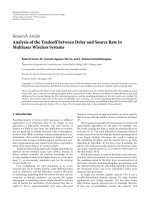
strict sense). In Figure 2, the cross-correlation function (up-
per diagram) and the predicted local maxima function (bot-
tom diagram) are illustrated for an omnidirectional source
located in the environment shown in Figure 1,andwhenu
is equal to “k” as uttered by a male speaker in an anechoic
chamber.ItcanbeseeninFigure 2 that at the places, where
p
x
1
,x
2
(k) predicts local maxima with relatively high probabil-
ity, local maxima appear in the cross-correlation function.
Figure 2 illustrates the effect of PHAT weighting as well. Cor-
relation computation on the whitened signals (dotted line in
Figure 2) highlights the reverberation effects by suppressing
correlation peaks caused by signal periodicity. In Figure 2,
squares on the cross-correlation function indicate places of
supposed local maxima where reverberation takes effect.
Local maxima of cross-correlation function (either
PHAT weighted or not) in Figure 2 are identified by a two-
digit code. The first digit identifies the code of the path
which has reached m
1
, while the second digit identifies the
path which has reached m
2
. The path code 1 indicates the
direct path (solid line in Figure 1); codes 2 and 3 are the
first-order reflections from reflectors r

1
and r
2
,respectively
(dashed lines in Figure 1); while code 4 is the second-order
reflection path (dotted line in Figure 1).
The probability function of local maxima in the cross-
correlation function (p
x
i
,x
j
(k)) depends on the properties of
the acoustic configuration, that is, the location of the sound
source and the location of reflector surfaces. Thus, by assum-
ing that the reflecting surfaces are fixed, in order to indicate
the source location, an additional suffix s has to be affixed to
p
x
i
,x
j
(k). Thus, p
s,x
i
,x
j
(k)referstop
x
i

,x
j
(k) when the source is
at location s.
4 EURASIP Journal on Advances in Signal Processing
−450 100 450 −450 100 450 −450 100 450 −450
Lag
−0.5
0
0.5
1
Correlation
1-4
1-3
1-2
3-4
3-3
1-1
3-2
2-4
3-1
2-3
4-4
2-2
4-3
4-2
2-1
4-1
p
x1,x2

p
x1,x2
with PHAT weighting
(a)
−450 100 450 −450 100 450 −450 100 450 −450
Lag
0
0.5
1
Local maxima
prediction
1-4
1-3
1-2
3-4
3-3
1-1
3-2
2-4
3-1
2-3
4-4
2-2
4-3
4-2
2-1
4-1
p
x1,x2
(b)

Figure 2: The cross-correlation function (upper) and its prediction of local maxima (lower).
3.1. Effect of source directivity
Until now, earlier studies about source localization have not
considered the directional characteristics of the source; how-
ever, by examining the effect of source directivity, several
phenomena can be explained. The relatively weak perfor-
mance of TDOA-based speaker localization systems used
currently is interpreted as the consequence of reverberation
that causes spurious peaks in the cross-correlation function,
since two reflected paths with the same propagation delay to
the microphone may add leading to a higher peak, result-
ing in false TDOA estimation. By taking source and micro-
phone directivity into account, the coincidence of time dif-
ference of reverberation paths is not a necessary condition
for the occurrence of false TDOA estimation. Due to the
joint effect of the source and microphone directivity, a less
attenuated reverberation path may result in a peak higher
than that of the direct path. Although in speaker localization
systems the application of omnidirectional microphones is
widely spread, the directional characteristic of mouth [28]
may lead to a difference of several dB in the level of attenu-
ation between different paths. The current attenuation level
depends on the spectral content of the speech uttered from
the mouth. Even so, as stated in the second section, we ap-
ply a frequency-independent model, thus the directivity of
mouth is modeled by a function which is independent of
the frequency. The attenuation to a given direction is consid-
ered to be the average of attenuation computed in the spec-
tral region of interest. Using this simplification, we can state
when

α

τ
d
, {}

<α

τ
r
, R
r

(12)
holds, the highest peak will not assign the true source loca-
tion. In expression (12), indices r and d denote any reflected
and direct path, respectively.
In Figure 3, the effect of source directivity of a hu-
man speaker in the environment in Figure 1 is illustrated.
The cross-correlation function and the probabilities of local
maxima in c
x
1
,x
2
(k) for 270
◦
head direction are depicted in
Figure 3. As it can be seen, the highest peak of the cross-
correlation function (3-3) gives a false TDOA, resulting

in bad location estimates in traditional TDOA-based algo-
rithms [6–11].
To find the correct TDOA, the directivity of nonisotropic
sound sources should be considered and the definition of
predicted local maxima function has to be extended to a
direction-specific form. The latter is given by p
s,φ,θ,x
i
,x
j
(k),
where s is the location of sound source, x
i
and x
j
refer to
the signals recorded by microphone i,andj, φ,andθ are the
azimuthal and elevation orientations of the source, respec-
tively.
A predicted local maxima function is to be created for
each microphone pair based on the given acoustic configura-
tion, that is, the location of sound source and microphones,
the direction of sound source, and the acoustic properties of
the environment. In fixed acoustic environment, the num-
ber of predicted local maxima functions is

N
2

·|C

A
|,where
N denotes the number of microphones and
|C
A
| is the car-
dinality of the set of possible acoustic configurations. C
A
contains triplets with general structure (s, φ, θ), where s is
the location of the sound source (s
∈ C), φ and θ are the
azimuth and elevation degrees of different source orienta-
tions. Obviously, in case of an isotropic sound source, ori-
entation does not need to be distinguished, that is,
|C
A
|=
|
C|.
Z. Fodr
´
oczi and A. Radv
´
anyi 5
−450 −350 −250 −150 −50 50 150 250 350 450
Lag
−0.5
0
0.5
1

Correlation
1-4
1-3
1-2
3-4
3-3
1-1
3-2
2-4
3-1
2-3
4-4
2-2
4-3
4-2
2-1
4-1
p
x1,x2
p
x1,x2
with PHAT weighting
(a)
−450 −350 −250 −150 −50 50 150 250 350 450
Lag
0
0.5
1
Local maxima
prediction

1-4
1-3
1-2
3-4
3-3
1-1
3-2
2-4
3-1
2-3
4-4
2-2
4-3
4-2
2-1
4-1
p
x1,x2
(b)
Figure 3: The effect of mouth directivity. The true TDOA is at (1-1).
4. AGGREGATE EFFECT OF THE ACOUSTIC
ENVIRONMENT
The proper accumulation of the local maxima predictions of
microphone pair combinations is essential for constructing a
robust and computationally efficient algorithm. An effective
method was published in [11], which follows the principle of
least commitment. It is effective as it delays the decision as
long as possible, resulting in more robust behavior. The idea
is to map the PHAT-weighted cross-correlation functions to
a common coordinate system according to

£(l)
=
N

i=1
N

j=i+1
c
x
i
,x
j

τ
i,l
−τ
j,l

, (13)
where £(l) is the likelihood that the source is at location
l(l
∈ C); τ
i,l
and τ
j,l
are the travel times of the sound wave
from location l to microphones i and j, respectively. In this
paper, we apply this idea to accumulate the local maxima pre-
dictions of the cross-correlation functions, thus we define

p
RM
s,φ,θ
(l) =
N

i=1
N

j=i+1
p
s,φ,θ,x
i
,x
j

τ
i,l
−τ
j,l

, (14)
where p
RM
(s,φ,θ)
(l) is the accumulated prediction of local max-
ima at location l for the acoustic setup (s, φ,θ)
∈ A
C
,in

which s is the location of the sound source, φ and θ its az-
imuth and elevation angles. Note that the probability of lo-
cal maxima in c
x
i
,x
j
(k) depends on the attenuation of de-
layed replicas caused by reverberation, thus p
RM
s,φ,θ
(l)could
also be referred to as the accumulated effect of reverberation
at location l, By computation of p
RM
s,φ,θ
(l) for every possible
source location point, the so-called accumulated predicted
reverberation-effect map (later referred to as predicted re-
verberation map) can be created, which is denoted by p
RM
s,φ,θ
.
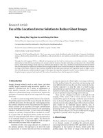
Figure 4 shows two predicted reverberation maps: one for the
arrangement in Figure 1 (left) and the other for the same ar-
rangement but with an additional microphone (right). The
source in this example is assumed to be omnidirectional.
The outstanding features of these maps are their local
maxima points. Thus a subset of local maxima points of pre-
dicted reverberation map is referred to as



p
RM
s,φ,θ
=

m ∈

p
RM
s,φ,θ
|p
RM
s,φ,θ
(m) >T
r
·max
c∈C

p
RM
s,φ,θ

c


,
(15)
where T

r
is a parameter denoting the lowest level of the pre-
dicted reverberation effect that needs to be considered,

p
RM
s,φ,θ
is the set of local maxima points. Note that, in the following
space, we will use “hat” sign (
·) to denote the local maxima
of an arbitrary map, while “double-hat” sign (

·
) will be used
to refer to the local maxima points which are above a certain
limit.
5. SOLVING THE INVERSE PROBLEM
In source localization practice, the inputs are records of
microphone signals from which a set of cross-correlation
functions can be computed. The cross-correlations can be
mapped to the monitored region as shown in (13). By
computing the likelihood for every possible source location
point, the accumulated correlation map (£) [11]canbecre-
ated, where £(l) refers to the likelihood of source at location
l.In[11], the location with the highest probability is selected
as the hypothetical source location point. In our approach,
we utilize this probability map but we defer the decision and
integrate the effect of reverberation as an additional cue to
make our estimation robust, as far as speaker direction is
concerned.

6 EURASIP Journal on Advances in Signal Processing
r
2
r
1
(a)
r
2
r
1
(b)
Figure 4: The predicted reverberation map. Rhombi show the places of microphones, and squares indicate the source location.
As we have shown, earlier reverberation causes local
maxima in the cross-correlation function. This information
is highlighted by applying PHAT weighting during cross-
correlation computation. Thus, by finding the local maxima
of the accumulated correlation map, the effect of reverbera-
tioncanbesummeduptodefine


£ =

m ∈

£ | £(m) >T
r
·£
max

, (16)

where

£ indicates the local maxima points of the accumulated
correlation map, T
r
is the parameter of the lowest limit of
significant reverberation effect, and £
max
= max
l∈C
{£(l)}.
5.1. Finding the prestored configuration which fits
observations best
In the previous sections, we have considered a method for
creating predictions and have discussed how to extract the ef-
fect of reverberation from our measurement. In the following
section, a similarity measure between predictions and obser-
vation is analyzed.
First, based on the accumulated correlation map (£), the
so-called feasible configuration set ( f
C
)iscreated.Themem-
bers of the feasible configuration set ( f
C
={(z, φ, θ) ∈
C
A
}⊂C
A
) are configurations, such that the accumulated

correlation value at the predicted maximum location (m
∈
C, p
RM
z,φ,θ
(m) = max
l∈C
{p
RM
z,φ,θ
(l)}) is close to the maximum of
the accumulated correlation map (£
max
·T
c
< £(m)), where
T
c
controls the acceptable difference compared to the max-
imum of accumulated correlation map (£
max
). In the fol-
lowing steps, selection of the most probable configuration
among these feasible configurations ( f
C
) will be discussed.
Note that both the selected local maxima of the predicted
reverberation maps (



p
RM
s,φ,θ
), which are stored for every possi-
ble configuration ((s, φ, θ)
∈ C
A
), and the selected local max-
ima of the accumulated correlation map (


£), which is com-
puted from the cross-correlation function, contain points
from the monitored region (C). In both cases, a value is as-
signed to every location of these maps ((p
RM
z,φ,θ
(l) | l ∈


p
RM
z,φ,θ
),
(£(l)
| l ∈


£)) describing their reliability. The number of pre-
dicted local maxima points (

|


p
RM
s,φ,θ
|) varies between different
configurations. The number of observed local maxima points
(|


£|) could also vary due to noise, thus the similarity of these
two point sets should be measured through global proper-
ties such as the center of gravity (P
cg
). As a consequence, the
matching of an observation to the elements of f
c
is computed
as
D(z, φ, θ)
=




P
cg




p
RM
z,φ,θ

−
P
cg



£





+




P
icg



p
RM
z,φ,θ


−
P
icg



£





,
(17)
where the first term shows the distance from the center of
gravities of the prediction (z,φ, θ) to that of the observation.
The computation of center of gravity on any M
∈{


p
RM
z,φ,θ
|
(z, φ, θ) ∈ f
C
}∪{



£} map can be carried out by evaluating
P
cg
(M) =

m∈M
(M(m)·T
TDOA
(m))

m∈M
M(m)
, (18)
where M(m) is the value of map M at location m
∈ M
and T
TDOA
(m) assigns an

N
2

-dimensional vector that cor-
responds to m in the TDOA space (
S
TDOA
), (T
TDOA
(m) ∈
S

TDOA
⊂ R

N
2

). T
TDOA
(·) assigns an operator that projects
an arbitrary location from C to
S
TDOA
as given by
T
TDOA
(m) =

χ
1
, χ
2
, , χ

N
2


T
, (19)
where

T
assigns the transpose operation, χ
k

k = 1
N
2

is the
kth coordinate in
S
TDOA
, which is equal to
χ
k
= τ
i,m
−τ
j,m
, (20)
Z. Fodr
´
oczi and A. Radv
´
anyi 7
where τ
i,m
and τ
j,m
are the travel times of the sound wave

from location m to microphones i and j,respectively.The
index pairs of the microphones (i, j) are selected as the kth
element of the list of all combinations of the microphone in-
dices.
The result of P
cg
(M) is a point in S
TDOA
which assigns
the center of gravity of map M. The second term in (17)is
thedistance between the so-called inverse center of gravity
(P
icg
) points where the inverse center of gravity of map (M)
is computed from
P
icg
(M) =

m∈M

M
max
−M(m)

·
T
TDOA
(m)



m∈M

M
max
−M(m)

, (21)
where M
max
is the maximum value of map M.
In (17),
· denotes the length of a vector in the TDOA
space which interconnects the points arising from either P
icg
or P
cg
, and can be computed as
v
TDOA
=

N
2


k=1

v
2

k
, (22)
where v
TDOA
∈ S
TDOA
and v
k
is the kth coordinate of v
TDOA
.
The hypothetical source location point determined by
the proposed method is the best matching configuration and
is selected as
min
(z,φ,θ)∈f
C

D(z, φ, θ)

. (23)
To sum up what is mentioned in the previous sections, we
extended the accumulated correlation algorithm for acoustic
localization. We have built offline maps that store the rever-
beration effect of different acoustic configurations. The ob-
servation gathered from the microphone records were com-
pared to these prestored maps to find the best match, which
yields the most likely source location.
6. EFFECT OF DISCRETIZATION
Theaboveequationsassumecontinuoustimeandanin-

finitely dense grid of possible source location points, which
are obviously not applicable in practice. By assuming that
all delays (τ
i,c
) can be adequately represented by an integer
number of sampling periods and by considering the Nyquist-
theorem, the continuous-time variables can be replaced by
their discretized equivalents. The question of spatial resolu-
tion of the accumulated correlation maps leads to the prob-
lem of time-delay imprecision or misalignment of beam-
formers [29]. The energy map of a beamformer is the visual
representation of variations in beamformer output energy
versus the coordinates of the point which the beamformer
is steered to. The source manifests itself as a peak in the en-
ergy map. The map depends on the array geometry and on
the spectral content of the signal. The width of the peak in
the energy map is, generally, smaller for higher-frequency
sources. In [29], it is shown that there exists an inverse re-
lationship between the peak width in the energy map and
the sound wavelength (λ); and it is conservatively estimated
that an error in the source position of less than λ/5 will still
result in a coherent gain in the beamformed signal. This re-
sult is referred to as imprecision heuristic. Since the accumu-
lated correlation map is essentially the same as the energy
map of beamformers [12], the imprecision heuristic can be
applied in our case as well. Based on this rule and by con-
sidering the maximum allowable spatial resolution, the max-
imum frequency of the sound signal usable for localization
can be determined. The same concept can be applied to map-
ping the predicted local maxima functions in (14). In this

case, p
x
i
,x
j
(k)shouldberedefinedas
p
x
i
,x
j
(k) =

p∈P
i

q∈P
j
a(τ
p
, R
p
)·a(τ
q
, R
q
)·Π(τ
p
−τ
q

−k),
(24)
where Π(τ
p
− τ
q
− k) is the value of the lowpass filtered
and shifted Dirac delta function at lag k. Lowpass filtering
of Dirac delta is carried out in compliance with imprecision
heuristic.
Using this modified version of predicted local maxima
function, the p
RM
s,φ,θ
maps can be created for the required res-
olutionin(14).
7. PERFORMANCE EVALUATION
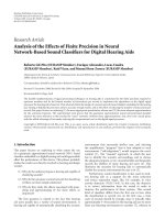
7.1. The test environment
In an attempt to evaluate the performance of the proposed
algorithm in a real-reverberant acoustic environment, an
acoustic model was built for an auditorium in P
´
azm
´
any
P
´
eter Catholic University (Budapest, Hungary) using the
CATT [30] Acoustic simulation software. In the three-
dimensional acoustic model of the auditorium (Figure 5)a

two-dimensional so-called source location plane was defined
parallel to the floor at 1.7 m, the average height of common
speakers. In practical applications where the height of speak-
ers varies, it could be necessary to define several source lo-
cation planes parallel to each other. However, in this paper,
we do not consider this a problem and assume the height of
the speaker to be constant at 1.7 m. The most significant en-
ergy portion of speech is around 500 Hz for male and around
700 Hz for female speakers, thus we choose 700 Hz as the
highest frequency used for localization. The spatial resolu-
tion was determined from imprecision heuristic [29]withres-
olution of 0.1 m. The set containing the possible source loca-
tion points (C) was created as nodes of a grid of 0.1 m density
defined on the source location plane.
The creation of the predicted local maxima functions
requires a priori the impulse response functions from ev-
ery possible source location points to the microphones. De-
termination of these impulse response functions by mea-
surements, due to their high number, could be problematic.
There are several acoustic modeling softwares [30, 31]avail-
able that can be used for predicting the impulse response
functions even in a very complex environment. In this work,
we have utilized the CATT Acoustic software. The elabora-
tion of the model can be determined along the guidelines de-
scribed in Section 8.1 by considering the highest frequency
8 EURASIP Journal on Advances in Signal Processing
(a) (b)
Figure 5: In the left figure, the 3D model of the simulated acoustic environment of the auditorium is depicted. The right figure is the photo
of the modeled auditorium.
012345678910

(m)
0
2
4
6
8
10
(m)
A
2
A
3
A
1
A
4
m
0
m
1
m
2
m
3
m
4
m
5
ϕ
Figure 6: Positions of microphones and the azimuth degree of the

speaker direction in the monitored auditorium.
used for localization. Based on these assumptions, we took
each object of spatial extent more than 1 m in any direction
into consideration. In each possible source location point, we
distinguished four different speaker directions, with 90
◦
ro-
tations of the azimuthal degree. The human mouth directiv-
ity data used for creating the impulse response functions was
created according to the results published in [28]byaverag-
ing the directivity data below 1 kHz. According to [28], we
may say that this approximation gives good results for sev-
eral speakers of different sex. Since the variation of the at-
tenuation level of the mouth is relatively independent of the
elevation angle of the head in the region of interest, we did
not distinguish different elevation angles, and it was fixed at
0
◦
to the source location plane. The location of the omni-
directional microphones and the interpretation of the head
direction are shown in Figure 6.
The above procedure resulted in 53891 different acoustic
configurations and 323346 impulse response functions. The
impulse responses were generated with a maximum of four
orders of specular reflections and the predicted local maxima
functions were created by considering the fifty strongest re-
flection paths based on (24) by assuming 25 kHz sampling
frequency. The

p

RM
and

£ sets were developed by applying
a series of gradient searches. For each run, the initial point
of the gradient search was chosen from a subset of C, whose
1077 points were equally distributed in the source location
plane. The calculation of all the impulse response functions
and the 53891 predicted reverberation-effect maps (


p
RM
)re-
quired less than one day for a Pentium IV class computer.
In each experiment, the maximum acceptable accumulated
correlation difference was set to 5%, and thus the value of
T
c
was 0.95 at the selection of feasible configuration set ( f
C
).
Performances of the algorithms were compared on a hypo-
thetical speaker path shown by a dashed line in Figure 6.In
the first part of the path (A
1
-A
2
), the speaker turns to the
wall and moves to point A

2
. This part aims at modeling a lec-
turer when writing on the blackboard, while speaking to the
audience. In the second (A
2
-A
3
) and the third part (A
3
-A
4
),
speech is directed to the direction of movement. On some
parts of this path, condition (12) holds which highlights the
extended capabilities of the proposed method; while other
parts aim at comparing performance in classical cases when
(12) does not hold.
7.2. Optimal level of considerable reverberation effect
In order to check the performance of the proposed method,
we divided the 27-second-long anechoic recording of an En-
glish male speaker into 40 segments. The sample rate of the
signal was 25 kHz, the length of each segment was 32768
samples, and the adjacent segments were overlapped with
16384 samples. The microphone signals were synthesized by
convolving these recordings with the generated impulse re-
sponses of points on the path shown in Figure 6. The impulse
responses used in convolution were generated with eight or-
ders of specular reflections. Performances of the accumulated
correlation and the proposed method were measured by us-
ing the 700 Hz lowpass filtered versions of the selected seg-

ments. In order to examine the global properties of different
T
r
parameters, we computed the root mean square (RMS) lo-
calization error along 178 points of the path, and have shown
the results in Figure 7.
Results show that the proposed method decreased the
RMS localization error compared with the accumulated
correlation method. The optimal value of the considered
Z. Fodr
´
oczi and A. Radv
´
anyi 9
5 152535455565758595
T
r
(%)
0
0.06
0.11
0.17
0.23
0.28
0.34
0.4
0.45
0.51
RMS localization error (m)
Proposed

Accumulated correlation
Figure 7: Performance of sound source localization algorithms re-
latedtopathinFigure 6.
Table 1: Performance of the accumulated and the proposed method
on different parts of the path.
Equation
(12) holds
Equation
(12)Does
not hold
Number of locations
134 44
RMS error of the accumulated
correlation [m]
0.58 0
RMS error of the proposed
method (T
r
= 55%) [m]
0.25 0.1
RMS error of the proposed
method (T
r
= 25%) [m]
0.3 0.06
reverberation effect is below 55%, because, above this limit,
it identifies the source location with more uncertainty. Be-
low this limit, the remaining localization error is caused by
the limited capabilities of the applied match measurement
induced by the information loss of center of gravities (see

Section 5.1). Taking even the smallest peaks into account (be-
low T
r
= 15%), the performance decreases because the peaks
caused by the deviation of the correlation values of the sig-
nals are considered to be the effects of reverberation.
Examining the results in Figure 8, a remarkable perfor-
mance difference can be observed between the two methods,
which originates from the parts of the path given when the
speaker faces the wall and the condition in (12)holds.On
the remaining portion of the path, both methods perform
basically the same as detailed in Tab le 1 . The slightly worse
performance of the proposed method when (12)doesnot
hold can be attributed to the imperfections of match mea-
surement detailed in Section 5.1.
7.3. Performance in noisy condition
The robustness of source localization algorithms in noisy
conditions is an important feature. Several previous studies
[2, 9, 32] on source localization, including this paper, assume
that noise is uncorrelated across the array although this as-
sumption does not hold in real environments. Correlating
noise fields lead to the improved model of the effect of real-
world pointlike noise sources such as computer fans, projec-
tors, and ceiling fans. However, few works [33, 34] succeeded
in extending the capabilities of existing methods to spatially
correlated noise with known statistics, due to its challeng-
ing complexity. The current work does not consider the cor-
related noise problem but examines the robustness of the
proposed method applied to uncorrelated noise fields. We
have added mutually uncorrelated Gaussian white noise to

the microphone inputs which were used in the previous sec-
tion. The resulting signals with 30 to
−10 dB signal-to-noise-
ratio (SNR) were used to compare the performance of the ac-
cumulated correlation method with the performance of the
proposed one with T
r
= 0.55 and T
r
= 0.25.
The results in Figure 9 show that for low-SNR values, the
proposed method gives slightly worse results. The reason is
that added noise causes additional local maxima in the cross-
correlation function. Since the effect of reverberation is con-
sidered through local property (i.e., local maximum), addi-
tional local maxima caused by added noise make the estima-
tion less reliable. A possible solution to this problem could
be the integration of the effect of reverberation in certain ar-
eas (see the lighter areas in Figure 4). However, the proper
integration of the effect of reverberation at acceptable speed
is not a trivial task, and it is not discussed in this work.
7.4. Performance in different acoustic environment
The performance evaluation of localization algorithms in
different reverberation conditions is a common practice [1–
14]. In this paper, we use reverberation as an additional cue
to make the localization more robust; thus in our case, this
task is interpreted as to evaluate localization performance in
varying acoustic conditions. The acoustic environment may
alter due to the effect of several factors [35] such as humidity,
temperature, location of reverberant/absorption surfaces. By

considering the typical application area of our algorithm, the
first two effects can be ignored since these parameters in ev-
eryday conference environment are considered to be constant
together with location and wrapping, that is, absorption co-
efficient of walls and furniture. However, the number of peo-
ple in the hall may vary from one person to full capacity of
the room, thus we have to evaluate the performance of our al-
gorithm as the function of the density of listeners in the audi-
torium. To analyze the effect of the audience size on the local-
ization performance, we used the acoustic model discussed
earlier. We have synthesized records based on the same path
(see Figure 6), but the absorption coefficient of the audience
area was changed to the measured values published in [36].
Using this method, we simulated a density of 2 person/m
2
in the audience area with changing reverberation time (T
30
)
of the auditorium from 3.5 seconds to 1.5 seconds. The lo-
calization was performed on microphone signals which were
synthesized by impulse responses of the altered room. The
results of this experiment are shown in Figure 10 where the
RMS localization error ratio of the proposed method with
T
r
= 55% to accumulated correlation is depicted. The figure
shows that the proposed method tolerates moderate changes
10 EURASIP Journal on Advances in Signal Processing
012345678910
(m)

0
2
4
6
8
10
(m)
(a)
012345678910
(m)
0
2
4
6
8
10
(m)
(b)
Figure 8: Localization results. The left figure shows results by the accumulated correlation method, while the right figure shows the results
through the proposed method with T
r
= 55%.
30 20 10 0 −10
SNR (dB)
0
0.2
0.4
0.6
0.8
1

1.2
1.4
1.6
1.8
RMS localization error (m)
Accumulated correlation
25
55
Figure 9: Effect of added Gaussian white noise on localization per-
formance.
30 20 10 0 −10
SNR (dB)
50
60
70
80
90
100
110
120
130
140
RMS localization error of proposed method
RMS localization error of accumulated correlation
(%)
2 person/sqm
Empty room
Figure 10: Localization performance in different acoustic condi-
tions.
in the acoustic environment, due to the fact that its perfor-

mance basically does not alter.
7.5. Speed of convergence
A conventional way of obtaining more reliable location esti-
mates is to aggregate the results of several measurements. The
speed of convergence of estimates to the true source location
could be an important issue in case of low-quality measure-
ments. In case of the algorithms in question, the accumula-
tion of results of different measurements is done through the
aggregation over time of accumulated correlation maps, thus
we redefine the notation of £(l)as
£(l)
=
L

i=L−S
£
i
(l)
∀l ∈ C
, (25)
where £
i
(l) is the accumulated correlation map of the ith
measurement computed according to (13)atlocationl,and
L is the sequence number of the last measurement. S con-
trols the number of previous measurements to be consid-
ered. The value of S should be set according to the several
parameters of application such as the maximum velocity of
the moving speaker, the sampling rate, or the length of win-
dowonwhichcorrelationiscomputed(2

·W). In our exper-
iments, we set S
= L to examine the convergence speed of
the proposed method. The results of localization algorithms
were checked at each location of the path shown in Figure 6.
The microphone signals applied in this experiment were syn-
thesized by applying the same anechoic recordings we used
earlier. In order to examine the evaluation of estimates along
the time axis, 27-second-long signals were created for each
location (i.e., the speaker spent 27 seconds in each location
on the path). The results of both methods were determined
after every 32768 samples of the microphone signals for each
location on the path. The RMS localization errors computed
for each location were averaged along the path in each time
instance with the results shown in Figure 11.
Z. Fodr
´
oczi and A. Radv
´
anyi 11
1.31
2.62
3.93
5.24
6.55
7.86
9.18
10.49
11.8
13.11

14.42
15.73
17.04
18.35
19.66
20.97
22.28
23.59
24.9
Length of signals, on which results of
measurements were aggregated (s)
0.2
0.25
0.3
0.35
0.4
0.45
0.5
0.55
0.6
0.65
RMS localization error (m)
Proposed (10 dB SNR)
Proposed (clean signal)
Accumulated correlation (10 dB SNR)
Accumulated correlation (clean signal)
Figure 11: Evaluation of location estimates by aggregating the re-
sults of several measurements.
The evaluation of location estimates was performed for
both clean and noisy signals with a 10 dB SNR.

The results show that the summation of results of several
measurements does not change the performance of the accu-
mulated correlation method, since the error caused by joint
effect of reverberation and source directivity holds for each
measurement. Moreover, it can be seen that a 10 dB SNR in
the recorded signals does not alter the performance of accu-
mulated correlation method. The examination of the results
of the proposed method on clean signals suggests that local-
ization error is independent on the signal length as its per-
formance does not change during the evaluation. Moreover,
it proves that the error of the proposed method is caused
by the imperfections of matching measurement between ob-
servation and predictions and the error incurred from spa-
tial discretization. Performance evaluation on noisy signals
shows that by averaging several measurements, the error in-
troduced by the added noise can be decreased, and the per-
formance of the proposed method can be slightly improved.
Nevertheless, it does not exceed the performance of the ac-
cumulated correlation method and the speed of convergence
is too slow to track speakers in practical applications.
8. DISCUSSION
8.1. Validity of the applied acoustic model
In our work, we have considered the frequency-independent
specular sound reflection model that has certain limitations.
Using the model in question, good approximations can be
achieved when the following conditions hold.
(i) The wavelength of the sound signal is significantly
shorter than the extent of the reflector.
(ii) The surface of the reflector can be considered to be pla-
nar compared to the sound wavelength.

(iii) There is no obstructing object along the propagation
path the extent of which would be comparable to the
wavelength.
Table 2: Approximation of frequencies where the applied acoustic
model gives good approximation of real-world effects.
Application
environment
Typical dimensions
(height
· width · depth)
Lowest frequency
range
Office room 3 m · 5m· 5m
2 kHz
Class room 3 m
· 10 m · 6m
1.5 kHz
Small
Auditorium
5m
· 15 m · 10 m
600 Hz
Conference
Hall
8m
· 30 m · 30 m
200 Hz
In cases when the first and the third conditions fail, the edge
diffraction effects should be considered, while failure of the
second condition implies the importance of modeling sound

scattering. By considering a typical conference environment
and application profile, we can assume that the third condi-
tion holds. The investigation of the remaining factors, how-
ever, is an active research area in computational acoustics.
Studies related to the problem [37–39] suggest that the early
part of reverberation can be well characterized by the specu-
lar reflection model. Since early reflections contain the main
portion of energy of the reverberated sound, the applied
model is considered suitable for predicting the most disturb-
ing peaks in the cross-correlation function that is caused by
delayed replicas of sound.
Based on the typical dimensions of the monitored re-
gion, the validity of specular reflection model can be evalu-
ated by considering the frequency of the sound signals which
are present. In our study, we considered four application
environments, listed in Ta b le 2 . In this table, we indicate
the lowest-frequency range above which the specular reflec-
tion model can be considered to be a good approximation
of the real world. For smaller enclosures, the results show
that only the higher frequency portion of speech can fit this
method. Consequently, the proposed method is more suit-
able for speaker localization in auditoriums and conference
halls.
8.2. Computational requirement
The speed of source localization algorithms is a crucial fac-
tor, because the typical application profile requires real-time
processing. In Tab le 3, we summarized the offline and real-
time computational requirement of the proposed procedure,
the accumulated correlation and the MFA-based methods.
The distinct advantage of the proposed method com-

pared to MFA-based ones is that there is no need to de-
convolve the input signal in real-time at each location of
the search space, since the effect of reverberation is offline
evaluated. On the other hand, this method carries moderate
computational overhead compared to the accumulated cor-
relation, owing to local maxima extraction and match mea-
surement. The effect of this latter factor can be controlled
through parameter T
c
creating a feasible configuration set. In
our experiments, the number of configurations in this set was
12 EURASIP Journal on Advances in Signal Processing
Table 3: Estimated computational requirement of different algorithms.
Algorithm Offline computation Real-time computation
Accumulated correlation
[11]
—
- Computation of cross-correlation function
- Mapping to a common coordinate system.
Delay-and-sum beamformer
- Computation of impulse response function for
each possible source location point
- Deconvolution of the input signal with the ap-
propriate impulse response function for every pos-
sible source location point
with MFA [20]
- Computation of beamformer response with the
deconvolved signals
Proposed method
- Computation ofimpulse response function for

each possible configuration
- Computation of cross-correlation functions
- Creation of predicted reverberation map for each
configuration
- Mapping to a common coordinate system
- Search for local maxima in each predicted map
- Search for local maxima
- Match measurement with a subset of stored
predictions
less than 100 in every case, leaving most of the computational
overhead to the gradient search process. Even though, creat-
ing the accumulated correlation map can be performed more
efficiently than the energy response map of beamformer, the
computational requirement of the proposes method is still
questionable in cases when three-dimensional search space
is considered.
9. CONCLUSION
In this work, a novel TDOA-based sound source localiza-
tion algorithm was presented which integrates a priori in-
formation of the acoustic environment for the localization
of directional sound sources in reverberant environments.
The algorithm utilizes the redundant information provided
by multiple sensors to enhance the TDOA performance.
By the support of the specular reflection model of sound
waves, more reliable localizations can be achieved in the
cases when the joint effect of source directivity and rever-
beration causes traditional methods to fail. The proposed
method results in significantly better estimates in case of
noise-free signals, while it performs worse in SNR’s signals
lower than 20 dB. We showed that integration of informa-

tion from the acoustic environment could be carried out
offline with reasonable real-time computational overhead.
The validity of the acoustic model applied and the per-
formance of the proposed algorithm in various simulated
acoustic conditions were discussed suggesting its usability
in conference environment. Although this work demon-
strated the importance of directional properties of sound
sources and showed an alternative localization framework
where a matching of observations to predicted quantities
was considered, speaker localization remains to be a diffi-
cult problem in a practical noisy environment. Further re-
search is stimulated by the results obtained in this direc-
tion to increase performance of source localization algo-
rithms using a priori information of the acoustic environ-
ment.
APPENDIX
By substituting (1)to(4), we get
R
x
i
,x
j
(k) = E


p∈P
i
a

τ

p
, R
p

·u

t −τ
p

+ η
i
(t)

·


q∈P
j
a

τ
q
, R
q

·u

t −τ
q
−k


+ η
j
(t −k)

,
R
x
i
,x
j
(k) = E


p∈P
i
a

τ
p
, R
p

·
u

t −τ
p



·


q∈P
j
a

τ
q
, R
q

·u

t −τ
q
−k


+ E


p∈P
i
a

τ
p
, R
p


·
u

t −τ
p


·
η
j
(t −k)

+ E


q∈P
j
a

τ
q
, R
q

·
u

t −τ
q

−k


·
η
i
(t)

+ E

η
i
(t)·η
j
(t −k)

;
(A.1)
as we assumed, the components are mutually uncorrelated,
thus the second, third, and the fourth expressions are ap-
proximately equal to zero if both signal and noise have zero-
mean and the equation can be rewritten as
R
x
i
,x
j
(k) =

p∈P

i

q∈P
j
a

τ
p
, R
p

·
a

τ
q
, R
q

·
E

u

t −τ
p

·u

t −τ

q
−k

,
(A.2)
which is equal to the weighted sum of the time-shifted auto-
correlation functions whose shift is equal to (τ
p
−τ
q
):
c
x
i
,x
j
(k) =

p∈P
i

q∈P
j
a

d
p
, R
p


·
a

d
q
, R
q

·
c
u,u

τ
p
−τ
q
−k

.
(A.3)
Z. Fodr
´
oczi and A. Radv
´
anyi 13
ACKNOWLEDGMENTS
Special thanks are due to Daniel V. Rabinkin for his audio
records that helped us during the development of the al-
gorithm, to Bengt-Inge Dalenback, head of CATT Acoustic,
for supporting the software for research, and to Dr. A. C. C.

Warnock for supplying directional data of the human mouth.
We also thank the anonymous reviewers for their valuable
comments. This project has been supported by the Hungar-
ian Scientific Research Fund OTKA-TS40858.
REFERENCES
[1] J. H. DiBiase, H. F. Silverman, and M. S. Branstein, “Robust
localization in reverberant rooms,” in Microphone Arrays: Sig-
nal Processing Techniques and Applications, M. S. Branstein and
D. B. Ward, Eds., chapter 8, pp. 157–180, Springer, New York,
NY, USA, 2001.
[2] J. Benesty, “Adaptive eigenvalue decomposition algorithm for
passive acoustic source localization,” Journal of the Acoustical
Society of America, vol. 107, no. 1, pp. 384–391, 2000.
[3] Y. Huang and J. Benesty, “A class of frequency-domain adap-
tive approaches to blind multichannel identification,” IEEE
Transactions on Signal Processing, vol. 51, no. 1, pp. 11–24,
2003.
[4] G. C. Carter, “Variance bounds for passively locating an acous-
tic source with a symmetric line array,” Journal of the Acoustical
Society of America, vol. 62, no. 4, pp. 922–926, 1977.
[5] D. B. Ward, E. A. Lehmann, and R. C. Williamson, “Particle
filtering algorithms for tracking an acoustic source in a rever-
berant environment,” IEEE Transactions on Speech and Audio
Processing, vol. 11, no. 6, pp. 826–836, 2003.
[6] J. P. Ianniello, “Time delay estimation via cross-correlation in
the presence of large estimation errors,” IEEE Transactions on
Acoustics, Speech, and Signal Processing, vol. 30, no. 6, pp. 998–
1003, 1982.
[7] M. Brandstein, J. E. Adcock, and H. Silverman, “Practical
time-delay estimator for localizing speech sources with a mi-

crophone array,” Computer Speech and Language,vol.9,no.2,
pp. 153–169, 1995.
[8] M. Brandstein, J. Adcock, and H. Silverman, “A closed-form
location estimator for use with room environment micro-
phone arrays,” IEEE Transactions on Speech and Audio Process-
ing, vol. 5, no. 1, pp. 45–50, 1997.
[9] M. Brandstein and H. Silverman, “Robust method for speech
signal time-delay estimation in reverberant rooms,” in Pro-
ceedings of IEEE International Conference on Acoustics, Speech,
and Signal Processing (ICASSP ’97), vol. 1, pp. 375–378, Mu-
nich, Germany, April 1997.
[10] P. Svaizer, M. Matassoni, and M. Omologo, “Acoustic source
location in a three-dimensional space using crosspower spec-
trum phase,” in Proceedings of IEEE International Conference
on Acoustics, Speech, and Signal Processing (ICASSP ’97), vol. 1,
pp. 231–234, 1997.
[11] S. T. Birchfield and D. K. Gillmor, “Fast Bayesian acoustic lo-
calization,” in Proceedings of IEEE International Conference on
Acoustic, Speech, and Signal Processing (ICASSP ’02), vol. 2, pp.
1793–1796, Orlando, Fla, USA, May 2002.
[12] S. T. Birchfield, “A unifying framework for acoustic localiza-
tion,” in Proceedings of the 12th European Signal Processing
Conference (EUSIPCO ’04), Vienna, Austria, September 2004.
[13] C. H. Knapp and G. C. Carter, “The generalized correlation
method for estimation of time delay,” IEEE Transactions on
Acoustics, Speech, and Signal Processing, vol. 24, pp. 320–327,
1976.
[14] M. S. Brandstein, “Pitch-based approach to time-delay esti-
mation of reverberant speech,” in Proceedings of IEEE Work-
shop on Applications of Signal Processing to Audio and Acoustics

(ASSP ’97), New Paltz, NY, USA, October 1997.
[15] A. St
´
ephenne and B. Champagne, “A new cepstral prefiltering
technique for estimating time delay under reverberant condi-
tions,” Signal Processing, vol. 59, no. 3, pp. 253–266, 1997.
[16] S. M. Griebel and M. S. Brandstein, “Microphone array source
localization using realizable delay vectors,” in Proceedings of
IEEE Workshop on Applications of Signal Processing to Audio
and Acoustics (ASSP ’01), pp. 71–74, New Paltz, NY, USA, Oc-
tober 2001.
[17] J. Chen, J. Benesty, and Y. Huang, “Robust time delay esti-
mation exploiting redundancy among multiple microphones,”
IEEE Transactions on Speech and Audio Processing, vol. 11,
no. 6, pp. 549–557, 2003.
[18] J. Benesty, J. Chen, and Y. Huang, “Time-delay estimation via
linear interpolation and cross correlation,” IEEE Transactions
on Speech and Audio Processing, vol. 12, no. 5, pp. 509–519,
2004.
[19] E. E. Jan, Parallel processing of large scale microphone arrays
for sound capture, Ph.D. thesis, Rutgers the State University of
New Jersey, New Brunswick, NJ, USA, 1995.
[20] R. J. Renomeron, D. V. Rabinkin, J. C. French, and J. L. Flana-
gan, “Small-scale matched filter array processing for spatially
selective sound capture,” in Proceedings of the 134th Meeting of
the Acoustical Societ y of America,SanDiego,Calif,USA,De-
cember 1997.
[21] J. B. Allen and D. A. Berkley, “Image method for efficiently
simulating small-room acoustics,” Journal of the Acoustical So-
ciety of America, vol. 65, no. 4, pp. 943–950, 1979.

[22] J. Borish, “Extension of the image model to arbitrary polyhe-
dra,” JournaloftheAcousticalSocietyofAmerica, vol. 75, no. 6,
pp. 1827–1836, 1984.
[23] H. F. Silverman, W. R. Patterson III, J. L. Flanagan, and D. V.
Rabinkin, “Digital processing system for source location and
sound capture by large microphone arrays,” in Proceedings of
IEEE International Conference on Acoustics, Speech, and Sig-
nal Processing (ICASSP ’97), vol. 1, pp. 251–254, Munich, Ger-
many, April 1997.
[24] N. Checka, K. Wilson, V. Rangarajan, and T. Darrell, “A prob-
abilistic framework for multi-modal multi-person tracking,”
in Proceedings of IEEE Workshop on Multi-Object Tracking
(WOMOT ’03), Madison, Wis, USA, June 2003.
[25] A. Krokstad, S. Strom, and S. Sørsdal, “Calculating the acousti-
cal room response by the use of a ray tracing technique,” Jour-
nal of Sound and Vibration, vol. 8, no. 1, pp. 118–125, 1968.
[26] P. Heckbert and P. Hanrahan, “Beam tracing polygonal ob-
jects,” in Proceedings of the 11th Annual Conference on Com-
puter Graphics (SIGGR APH ’84), vol. 18, no. 3, pp. 119–127,
Minneapolis, Minn, USA, July 1984.
[27] T. Funkhouser, I. Carlbom, G. Elko, G. Pingali, M. Sondhi, and
J. West, “Beam tracing approach to acoustic modeling for in-
teractive virtual environments,” in Proceedings of the Annual
Conference on Computer Graphics (SIGGRAPH ’98), pp. 21–
32, Orlando, Fla, USA, July 1998.
[28] W. T. Chu and A. C. C. Warnock, “Detailed directivity of
sound fields around human talkers,” IRC Research Report
IRC-RR-104, National Research Council of Canada, Ottawa,
Ontario, Canada, 2002.
14 EURASIP Journal on Advances in Signal Processing

[29] D. N. Zotkin and R. Duraiswami, “Accelerated speech source
localization via a hierarchical search of steered response
power,” IEEE Transactions on Speech and Audio Processing,
vol. 12, no. 5, pp. 499–508, 2004.
[30] CATT-Acoustic .
[31] Odeon Room Acoustic Software .
[32] F. Talantzis, A. G. Constantinides, and L. C. Polymenakos,
“Estimation of direction of arrival using information theory,”
IEEE Signal Processing Letters, vol. 12, no. 8, pp. 561–564, 2005.
[33] Y. Rui and D. Florencio, “Time delay estimation in the pres-
ence of correlated noise and reverberation,” in Proceedings of
IEEE International Conference on Acoustics, Speech, and Sig-
nal Processing (ICASSP ’04), vol. 2, pp. II133–II136, Montreal,
Canada, May 2004.
[34] S. Doclo and M. Moonen, “Robust adaptive time delay estima-
tion for speaker localization in noisy and reverberant acoustic
environments,” EURASIP Journal on Applied Signal Processing,
vol. 2003, no. 11, pp. 1110–1124, 2003.
[35] L. E. Kinsler, A. R. Frey, A. B. Coppens, and J. V. Sanders,
Fundamentals of Acoustics, John Wiley & Sons, New York, NY,
USA, 1962.
[36] L. Karlen, Akustik i rum och byggander, Svensk Byggtj
¨
anst,
Stockholm, Sweden, 1983.
[37] N. Tsingos, I. Carlbom, G. Elko, R. Kubli, and T. Funkhouser,
“Validating acoustical simulations in the Bell Labs Box,” IEEE
Computer Graphics and Applications, vol. 22, no. 4, pp. 28–37,
2002.
[38] M. Kleiner, R. Orlowski, and J. Kirszenstein, “Comparison be-

tween results from a physical scale model and a computer im-
age source model for architectural acoustics,” Applied Acous-
tics, vol. 38, no. 2–4, pp. 245–265, 1993.
[39] L. L. Beranek, Concert and Opera Halls: How They Sound,
American Institute of Physics, Woodbury, NY, USA, 1996.