Báo cáo hóa học: " Research Article A Robust Structural PGN Model for Control of Cell-Cycle Progression Stabilized by Negative Feedbacks" pdf

Hindawi Publishing Corporation
EURASIP Journal on Bioinformatics and Systems Biology
Volume 2007, Article ID 73109, 11 pages
doi:10.1155/2007/73109
Research Article
A Robust Structural PGN Model for Control of Cell-Cycle
Progression Stabilized by Negative Feedbacks
Nestor Walter Trepode,
1
Hugo Aguirre Armelin,
2
Michael Bittner,
3
Junior Barrera,
1
Marco Dimas Gubitoso,
1
and Ronaldo Fumio Hashimoto
1
1
Institute of Mathematics and Statistics, University of S
˜
ao Paulo, Rua do Matao 1010, 05508-090 S
˜
ao Paulo, SP, Brazil
2
Institute of Chemistry, University of S
˜
ao Paulo, Avenue Professor Lineu Prestes 748, 05508-900 S
˜
ao Paulo, SP, Brazil

3
Translational Genomic s Research Institute, 445 N. Fifth Street, Phoenix, AZ 85004, USA
Received 27 July 2006; Revised 24 November 2006; Accepted 10 March 2007
Recommended by Tatsuya Akutsu
The cell division cycle comprises a sequence of phenomena controlled by a stable and robust genetic network. We applied a prob-
abilistic genetic network (PGN) to construct a hypothetical model with a dynamical behavior displaying the degree of robustness
typical of the biological cell cycle. The structure of our PGN model was inspired in well-established biological facts such as the
existence of integrator subsystems, negative and positive feedback loops, and redundant signaling pathways. Our model represents
genes interactions as stochastic processes and presents strong robustness in the presence of moderate noise and parameters fluctu-
ations. A recently published deterministic yeast cell-cycle model does not perform as well as our PGN model, even upon moderate
noise conditions. In addition, self stimulatory mechanisms can give our PGN model the possibility of having a p acemaker activity
similar to the observed in the oscillatory embryonic cell cycle.
Copyright © 2007 Nestor Walter Trepode et al. This is an open access article distributed under the Creative Commons Attribution
License, which permits unrestricted use, distribution, and reproduction in any medium, provided the original work is properly
cited.
1. INTRODUCTION
A complex genetic network is the central controller of the
cell-cycle process, by which a cell grows, replicates its genetic
material, and divides into two daughter cells. The cell-cycle
control system shows adaptability to specific environmental
conditions or cell types, exhibits stability in the presence of
variable excitation, is robust to parameter fluctuation and is
fault tolerant due to replications of network structures. It also
receives information from the processes b eing regulated and
is able to arrest the cell cycle at specific “checkpoints”ifsome
events have not been correctly completed. This is achieved by
means of intracellular negative feedback signals [1, 2].
Recently, two models were proposed to describe this con-
trol system. After exhaustive literature studies, Li et al. pro-
posed a deterministic discrete binary model of the yeast

cell-cycle control system, completely based on documented
data [3]. They studied the signal wave generated by the
model, that goes through all the consecutive phases of the
cell-cycle progression, and verified, by simulation, that al-
most all the state transitions of this deterministic model con-
verge to this “biological pathway,” showing stabilit y under
different activation signal waveforms. Based on experimental
data, Pomerening et al. proposed a continuous determinis-
tic model for the self-stimulated embryonic cell-cycle, which
performs one division after the other, without the need of
external stimuli nor waiting to grow [4].
We recently proposed the probabilistic genetic network
(PGN) model, where the influence between genes is repre-
sented by a stochastic process. A PGN is a particular family
of Markov Chains with some additional properties (axioms)
inspired in biological phenomena. Some of the implications
of these axioms are: stationarity; all states are reachable; one
variable’s transition is conditionally independent of the other
variables’ transitions; the probability of the most probable
state trajectory is much higher than the probabilities of the
other possible trajectories (i.e., the system is almost deter-
ministic); a gene is seen as a nonlinear stochastic gate whose
expression depends on a linear combination of activator and
inhibitory signals and the system is built by compiling these
elementary gates. This model was successfully applied for de-
signing malaria parasite genetic networks [5, 6].
Here we propose a hypothetical structura l PGN model
for the eukaryote control of cell-cycle progression, that aims
2 EURASIP Journal on Bioinformatics and Systems Biology
to reproduce the typical robustness observed in the dynam-

ical behavior of biological systems. Control structures in-
spired in well-known biological facts, such as the existence of
integrators, negative and positive feedbacks, and biological
redundancies, were included in the model architecture. Af-
ter adjusting its parameters heuristically, the model was able
to represent dynamical properties of real biological systems,
such as sequential propagation of gene expression waves, sta-
bility in the presence of variable excitation and robustness in
the presence of noise [7].
We carried out extensive simulations—under different
stimulus and noise conditions—in order to analyze stability
and robustness in our proposed model. We also analyzed the
performance of the yeast cell cycle control model constructed
by Li et al. [3] under similar simulations. Under small noisy
conditions, our PGN model exhibited remarkable robustness
whereas Li’s yeast-model did not perform that well. We in-
fer that our PGN model very likely possesses some structur a l
features ensuring robustness which Li’s model lacks. To fur-
ther emulate cellular environment conditions, we extended
our model to include random delays in its regulatory signals
without degrading its previous stabilit y and robustness. Fi-
nally, with the addition of positive feedback, our model be-
came self-stimulated, showing an oscillatory behavior simi-
lar to the one displayed by the embryonic cell-cycle [4]. Be-
sides being able to represent the observed behavior of the
other two models, our PGN model showed strong robustness
to system parameter fluctuation. The dynamical structure of
the proposed model is composed of: (i) prediction by an al-
most deterministic stochastic rule (i.e., gene model), and (ii)
stochastic choice of an almost deterministic stochastic pre-

diction rule (i.e., random delays).
After this introduction, in Section 2, we present our
mathematical modeling of a gene regulatory network by a
PGN. In Section 3, we br iefly describe Li’s yeast cell-cycle
model and present the simulation, in the presence of noise,
of our PGN version of it. Sections 4 and 5 describe the archi-
tecture and dynamics of our model for control of cell-cycle
progression and analyze its simulations in the presence of
noise and random delays in the regulatory signals (the same
noise pattern was applied to both our model and Li’s yeast-
model). Section 6 shows the inclusion of positive feedback in
our model to obtain a pacemaker activity, similar to the one
found in embryonic cells. Finally, in Section 7 we discuss our
results and the continuity of this research.
2. MATHEMATICAL MODELING OF
GENETIC NETWORKS
2.1. Genetic regulatory networks
The cell cycle control system is a complex network com-
prising many forward and feedback signals acting at specific
times. Figure 1 is a schematic representation of such a net-
work, usually called a gene regulatory network. Proteins pro-
duced as a consequence of gene expression (i.e., after tran-
scription and translation) form multiprotein complexes, that
interact with each other, integrating extracellular signals—
not shown—, regulating metabolic pathways (arrow 3), re-
DNA RNA Proteins
Metabolic
pathways
3
4

Transcription Translation
1
2
Feedback signals
Microa rray measurements
Figure 1: Gene regulatory network.
ceiving (arrow 4) and sending (arrow 1 and 2) feedback sig-
nals. In this way, genes and their protein products form a sig-
naling network that controls function, cell division cycle, and
programmed cell death. In that network, the level of expres-
sion of ea ch gene depends on both its own expression value
and the expression values of other genes at previous instants
of time, and on previous external stimuli. This kind of in-
teractions between genes forms networks that may be ver y
complex. The dynamical behavior of these networks can be
adequately represented by discrete stochastic dynamical sys-
tems. In the following subsections, we present a model of this
kind.
2.2. Discrete dynamical systems
Discrete dynamical systems, discrete in time and finite in
range, can model the behavior of gene networks [8–12]. In
this model, we represent each gene or protein by a variable
which takes the value of the gene expression or the protein
concentration. All these variables, taken collectively, are the
components of a vector called the state of the system. Each
component (i.e., gene or protein) of the state vector has as-
sociated a function that calculates its next value (i.e., expres-
sion value or protein concentration) from the state at previ-
ous instants of t ime. These functions are the components of
a function vector, called transition function, that defines the

transition from one state to the next and represents the actual
regulatory mechanisms.
Let R be the range of all state components. For example,
R
={0, 1} in binary systems, R ={−1, 0, 1} or R ={0, 1, 2}
in three levels systems. The transition function φ,foranet-
work of N variables and memory m, is a function from R
mN
to R
N
. This means that the transition function φ maps the
previous m states, x(t
− 1), x(t − 2), , x(t − m), into the
state x(t)withx(t)
= [x
1
(t), x
2
(t), , x
N
(t)]
T
∈ R
N
. A dis-
crete dynamical system is given by, for every time t
≥ 0,
x( t)
= φ


x( t − 1), x(t − 2), , x(t − m)

. (1)
A component of x is a value x
i
∈ R. Systems defined as above
are time translation invariant, that is, the transition function
is the same for all discrete time t. The system architecture—
or structure—is the wi ring diagram of the dependencies
Nestor Walter Trepode et al. 3
between the variables (state vector components). The system
dynamics is the temporal evolution of the state vector, given
by the transition function.
2.3. Probabilistic genetic networks
When the transition function φ is a stochastic funct ion (i.e.,
foreachsequenceofstatesx(t
− m), , x(t − 2), x(t − 1),
the next state x(t) is a realization of a random vector), the
dynamical system is a stochastic process. Here we repre-
sent gene regulatory networks by stochastic processes, where
the stochastic transition function is a particular family of
Markov chains, that is called probabilistic genetic network
(PGN).
Consider a sequence of random vectors X
0
, X
1
, X
2
,

assuming values in R
N
, denoted, respectively, x(0), x(1),
x(2), Asequenceofrandomstates(X
t
)
∞
t=0
is called a
Markov chain if for every t
≥ 1,
P

X
t
= x(t) | X
0
= x(0), , X
t−1
= x(t − 1)

=
P

X
t
= x(t) | X
t−1
= x(t − 1)


.
(2)
That is, the conditional probability of the future event, given
the past history, depends only upon the last instant of time.
Let X, with realization x, represent the state before a tran-
sition, and let Y , with realization y be the first state after
that transition. A Markov chain is characterized by a transi-
tion matrix π
Y|X
of conditional probabilities between states,
whose elements are denoted p
y|x
, and the probability distri-
bution π
0
of the random vector representing the initial state.
The stochastic transition function φ at time t,isgivenby,for
every t
≥ 1,
φ[x]
= φ

x( t − 1)

= y,(3)
where y is a realization of a random vector with distribution
p
•|x
.
An m order Markov chain—which depends on the m

previous instants of time—is equivalent to a Markov chain
whose states have dimension m
× N.
Let the sequence X
= X
t−1
, , X
t−m
with realization x =
x( t−1), , x(t−m) represent the sequence of m states before
a transition. A probabilistic genetic network (PGN) is an m
order Markov chain (π
Y|X
, π
0
) such that
(i) π
Y|X
is homogeneous, that is, p
y|x
is independent of t,
(ii) p
y|x
> 0 for all states x ∈ R
mN
, y ∈ R
N
,
(iii) π
Y|X

is conditionally independent, that is, for all states
x
∈ R
mN
, y ∈ R
N
,
p
y|x
= Π
N
i
=1
p

y
i
| x

,(4)
(iv) π
Y|X
is almost deterministic, that is, for every sequence
of states x
∈ R
mN
, there exists a state y ∈ R
N
such that
p

y|x
≈ 1,
(v) for every variable i there exists a matrix a
i
and a vector
b
i
of real numbers such that, for every x, z ∈ R
mN
and
y
i
∈ R if
N

j=1
m

k=1
a
k
ji
x
j
(t − k) =
N

j=1
m


k=1
a
k
ji
z
j
(t − k),
p
i

k=1
b
k
i
x
i
(t − k) =
p
i

k=1
b
k
i
z
i
(t − k),
then p

y

i
| x

=
p

y
i
| z

,0≤ p
i
≤ m.
(5)
These axioms imply that each variable x
i
is characterized
byamatrixandavectorofcoefficients and a stochastic func-
tion g
i
from Z, a subset of integer numbers, to R.
If a
k
ji
is positive, then the target variable x
i
is activated
by the variable x
j
at time t − k,ifa

k
ji
is negative, then it is
inhibited by variable x
j
at time t − k,ifa
k
ji
is zero, then it is
not affected by variable x
j
at time t − k. We say that variable
x
i
is predicted by the variable x
j
when some a
k
ji
is different
from zero. Similarly, if b
k
i
is zero, the value of x
i
at time t is
not affectedforitspreviousvalueattimet
− k. The constant
parameter p
i

, for the state variable x
i
, represents the number
of previous instants of time at which the values of x
i
can affect
the value of x
i
(t). If p
i
= 0, previous values of x
i
have no
effect on the value of x
i
(t) and the summation

p
i
k=1
b
k
i
x
i
(t −
k)isdefinedtobezero.
The component i of the stochastic transition function φ,
denoted φ
i

, is built by the composition of a stochastic func-
tion g
i
with two linear combinations: (i) a
i
and the previ-
ous states x(t
− 1), , x(t − m), and (ii) b
i
and the values of
x
i
(t − 1), , x
i
(t − p
i
). This means that, for every t ≥ 1,
φ
i

x( t − 1), , x(t − m)

= g
i
(α, β), (6)
where
α
=
N


j=1
m

k=1
a
k
ji
x
j
(t − k), β =
p
i

k=1
b
k
i
x
i
(t − k)(7)
and g
i
(α, β) is a realization of a random variable in R,with
distribution p(
•|α, β). This restriction on g
i
means that the
components of a PGN transition function vector are random
variables with a probability distribution conditioned to two
linear combinations, α and β, from the fifth PGN axiom.

The PGN model reflects the properties of a gene as a non-
linear stochastic gate. Systems are built by compiling these
gates.
Biological rationale for PGN axioms
The axioms that define the PGN model are inspired by bio-
logical phenomena. The dynamical system structure is justi-
fied by the necessity of representing a sequential process. The
discrete representation is sufficient since the interactions be-
tween genes and proteins occur at the molecular level [13].
The stochastic aspects represent perturbations or lack of de-
tailed knowledge about the system dynamics. Axiom (i) is
4 EURASIP Journal on Bioinformatics and Systems Biology
just a constraint to simplify the model. In general, real sys-
tems are not homogeneous, but may be homogeneous by
parts, that is, in time intervals. Axiom (ii) imposes that all
states are reachable, that is, noise may lead the system to
any state. It is a quite general model that reflects our lack
of knowledge about the kind of noise that may affect the sys-
tem. Axiom (iii) implies that the prediction of each gene can
be computed independently of the prediction of the other
genes, which is a kind of system decomposition consistent
with what is observed in nature. Axiom (iv) means that the
system has a main trajectory, that is, one that is much more
probable than the others. Axiom (v) means that genes act as a
nonlinear gate triggered by a balance between inhibitory and
excitatory inputs, analogous to neurons.
3. YEAST CELL-CYCLE MODEL
The eukaryotic cell-cycle process is an ordered sequence of
events by which the cell grows and divides in two daugh-
ter cells. It is organized in four phases: G

1
(the cell progres-
sively grows and by the end of this phase becomes irreversibly
committed to division), S (phase of DNA synthesis and chro-
mosome replication), G
2
(bridging “gap” between S and M),
and M (period of chromosomes separation and cell division)
[1, 2]. The cell-cycle basic organization and control system
have been highly conserved during evolution and are essen-
tially the same in all eukaryotic cells, what makes more rele-
vant the study of a simple organism, like yeast.
We made studies of stability and robustness on a re-
cently published deterministic binary control model of the
yeast cell-cycle, which was entirely built from real biologi-
cal knowledge after extensive literature studies [3]. From the
≈ 800 genes involved in the yeast cell-cycle process [14],
only a small number of key regulators, responsible for the
control of the cell-cycle process, were selected to construct
a model where each interaction between its variables is doc-
umented in the literature. A dynamic model of these inter-
actions would involve various binding constants and rates
[15, 16], but inspired by the on-off characteristic of many
of the cell-cycle control network components, and focusing
mainly on the overall dynamic properties and stability, they
constructed a simple discrete binary model. In this work we
refer to its simplified version, whose architecture is shown in
Figure 1B of [3].
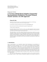
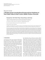
The simulation
1

in Figure 2(a) shows the state variables’
temporal evolution over the biological pathway, that goes
through all the sequential phases of the cell cycle, from the
excited G
1
state (activated when CS—cell size—grows be-
yond a certain threshold), to the S phase, the G
2
phase, the M
phase, and finally to the stationary G
1
state where it remains.
The cell-cycle sequence has a total length of 13 discrete time
steps (period of the cycle). Under simulations driven by CS
pulses of increasing frequency,
2
this system behaved well,
1
All simulations in this work were performed using SGEN (simulator for
gene expression networks) [17].
2
Simulations are not show n here.
0 4 8 1216202428
Time steps
CS 0
1
Cln30
1
MBF 0
1

SBF 0
1
Cln12 0
1
Cdh10
1
Swi50
1
Cdc20Cdc14 0
1
clb56 0
1
Sic10
1
Clb12 0
1
Mcm1SFF 0
1
State variables
(a) Simulation of the deterministic binary yeast cell-cycle model with
only one activator pulse of CS
= 1att =−1. After the START state
at t
= 0, the system goes through the biological pathway, passing by
all the sequential cell-cycle phases: G
1
at t = 1, 2, 3; S at t = 4; G
2
at
t

= 5; M at t = 6, , 10; G
1
at t = 11; and from t = 12 the system
remains in the G
1
stationary state (all variables at zero level except
Sic1
= Cdh1 = 1)
0 30 60 90 120 150 180
Time steps
CS 0
2
Cln30
2
MBF 0
2
SBF 0
2
Cln12 0
2
Cdh10
2
Swi50
2
Cdc20Cdc14 0
2
clb56 0
2
Sic10
2

Clb12 0
2
Mcm1SFF 0
2
State variables
(b) Simulation of the three-level PGN yeast cell-cycle model with 1%
of noise (PGN with P
= .99) activated by a single pulse of CS = 2at
t
=−1. After 13 time steps (period of the cycle), the system should
remain in the G
1
stationary state—all variables at zero level except
Sic1
= Cdh1 = 2—(compare with Figure 2(a)). Instead, this small
amount of noise is enough to take the system completely out of its
expected n ormal behavior
Figure 2: Yeast cell-cycle model simulations.
showing strong stability, with all initiated cycles systemati-
cally going to conclusion, and new cycles being initiated only
after the previous one had finished.
3.1. PGN yeast cell-cycle model
In order to study the effect of noise and the increase of the
number of signal levels in the performance of Li’s yeast-
model [3], we translated it into a three level PGN model. Ini-
tially, we mapped Li’s binar y deterministic model into a three
Nestor Walter Trepode et al. 5
Table 1: Threshold values for variables without self-degradation in
the PGN yeast cell-cycle model.
x

i
(t − 1) = 0 x
i
(t − 1) = 1 x
i
(t − 1) = 2
th
(1)
x
i
10−1
th
(2)
x
i
21 0
level deterministic one, with range of values R ={0, 1, 2} for
the state variables. By PGN axiom (iv), the PGN transition
matrix π
Y|X
is almost deterministic, that is, at every time step,
one of the transition probabilities p
y|x
≈ 1. The determinis-
tic case would be the case when, at e very time step, this most
probable transition have p
y|x
→ 1, or, in real terms, the case
corresponding to total absence of noise in the system. In this
mapping, binary value 1 was mapped to 2, and binary value 0

was mapped to 0, of the three-level model. Intermediate val-
ues (in the driving and transition functions) were mapped
in a convenient way, so that they lay between the ones that
have an exact correspondence. From this deterministic three-
level model (having exactly the same dynamical behavior of
the binary model from which it was derived) we specified the
following PGN.
3.1.1. PGN specification and simulation
The total input signal driving a generic variable x
i
(t) ∈
{
0, 1, 2} (1 ≤ i ≤ N)isgivenbyitsassociateddriving func-
tion:
d
i
(t − 1) =
N

j=1
a
ji
x
j
(t − 1). (8)
Here, the system has memor y m
= 1anda
ji
is the weight for
variable x

j
at time t − 1 in the driving function of variable
x
i
.Ifvariablex
j
is an activator of variable x
i
, then a
ji
= 1;
if variable x
j
is an inhibitor of variable x
j
, then a
ji
=−1;
otherwise, a
ji
= 0.
Let
y
i
(t) =
⎧
⎪
⎪
⎪
⎪

⎨
⎪
⎪
⎪
⎪
⎩
2ifd
i
(t − 1) ≥ th
(2)
x
i
,
1ifth
(1)
x
i
≤ d
i
(t − 1) < th
(2)
x
i
,
0ifd
i
(t − 1) < th
(1)
x
i

.
(9)
The stochastic transition function chooses the next value of
each variable to be (i) x
i
(t) = y
i
(t)withprobabilityP ≈ 1,
(ii) x
i
(t) = a with probability (1 − P)/2, or (iii) x
i
(t) = b
with probability (1
− P)/2; where a, b ∈{0, 1, 2}−{y
i
} and
th
(1)
x
i
,th
(2)
x
i
are the threshold values for one and two in the
transition function of variable x
i
. For this model to converge,
when P

→ 1, to the deterministic one in the previous sub-
section, these thresholds must have the values indicated in
Tab le 1 , depending on the value of x
i
(t − 1). If variable x
i
has
the self degradation property, its threshold values are those
in the column of x
i
(t − 1) = 0, regardless of the actual value
of x
i
(t − 1).
We simulated the three-level PGN version of Li’s yeast-
model with probability P
= 0.99 to represent the presence
of 1% of noise in the system. Figure 2(b) shows a 200 steps
simulation of the system when the G
1
stationary state is acti-
vated by a single start pulse of CS
= 2att =−1. Comparing
with Figure 2(a), we observe that this moderate noise is suf-
ficient to degrade the systems’ performance. Particularly, the
system should remain in the G
1
stationary state after the 13
steps cycle period, however, numerous spurious waveforms
are generated. Furthermore, when we simulated this system

increasing the frequency of the CS activator pulses, noise se-
riously disturbed the normal signal wave propagation [18].
We conclude that this system does not have a robust perfor-
mance under 1% of noise.
4. OUR STRUCTURAL MODEL FOR CONTROL OF
CELL-CYCLE PROGRESSION
The PGN was applied to construct a hypothetical model
based on components and structural features found in bi-
ological systems (integrators, redundancy, positive forward
signals, positive and negative feedback signals, etc.) having
a dynamical behavior (waves of control signals, stability to
changes in the input signal, robustness to some kinds of
noise, etc.) similar to those observed in real cell-cycle con-
trol systems.
During cell-cycle progression, families of genes have ei-
ther brief or sustained expression during specific cell-cycle
phases or transitions between phases (see, e.g., Figure 7 in
[14]). In mammalian cells, the transition G
0
/G
1
of cell cy-
cle requires sequential expression of genes encoding fami-
lies of master transcription factors, for instance the fos and
jun families of proto-oncogenes. Among the fos genes c-fos
and fos B are essentially regulated at transcription level and
are expressed for a brief period of time (0.5 to 1 h), dis-
playing mRNAs and proteins of very short half life. In ad-
dition, G
1

progression and G
1
/S transition are controlled by
the cell cycle regulatory machine, comprised by proteins of
sustained (cyclin-dependent kinases—CDKs—and Rb pro-
tein) and transient expression (cyclins D and E). The genes
encoding cyclins D and E are transcribed at middle and late
G
1
phase, respectively. Actually, there are several CDKs regu-
lating progression along all cell cycle phases and transitions,
whose activities a re dependent on cyclins that are transiently
expressed following a rigid sequential order. This basic regu-
lation of cell cycle progression is highly conserved in eukary-
otes, from yeast to mammalians. Accordingly, we organized
our model into successive gene layers expressed sequentially
in time. This wave of gene expression controls timing and
progression through the cell-cycle process.
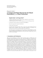
The architecture of our cell-cycle control model is de-
picted in Figure 3, showing the forward and feedback reg-
ulatory signals between gene layers (s, T, v, w, x, y,and
z), that determine the system’s dynamic behavior. These
gene layers represent consecutive stages taking place along
the classical cell-cycle phases G
1
, S, G
2
,andM. These lay-
ers are comprised by the genes—state variables—expressed
during the execution of each stage and are grouped into

the two main parts: (i) G
1
phase—layer s—that represents
the cell growth phase immediately before the onset of DNA
6 EURASIP Journal on Bioinformatics and Systems Biology
Time
G
1
phase S, G
2
and M phases
sTvwxyzGene layers
External
stimuli
s
1
s
2
s
5
F
T
Trigger gen e
F: integration of signals
from layer s
.
.
.
.
.

.
v
w
1
w
2
y
2
x
6
y
1
z
x
1
Forward signal
Feedback to T
Feedback to previous layer
Figure 3: Cell-cycle network architecture.
replication (i.e., S phase), during which the cell responds to
external regulatory stimuli (I) and (ii) S, G
2
plus M phases—
layers T, v, w, x, y,andz—that goes from DNA replication to
mitosis. The S phase trigger gene T represents an important
cell-cycle checkpoint, interfacing G
1
phase regulatory signals
and the initiation of DNA replication. The signal F (Figure 3)
stands for integration, at the trigger gene T,ofactivatorsig-

nals from layer s. Our basic assumption implies that the cell-
cycle control system is comprised of modules of parallel se-
quential waves of gene expression (layers s to z) organized
around a check-point (trigger gene T) that integrates for-
ward and feedback signals. For example, within a module,
the trigger gene T balances forward and feedback signals to
avoid initiation of a new wave of gene expression while a
first one is still going through the cell cycle. A number of
check-point modules, across cell cycle, regulate cell growth
and genome replication during the sequential G
1
, S,andG
2
phases and cell duplication via mitosis.
In our model, the expression of one of the genes in layers
v to z (i.e., after the trigger gene T—see Figure 3) typically
yields three types of signals in the system: (i) a forward acti-
vator signal to genes in the next layer that tends to make the
cell-cycle progress in its sequence; (ii) an inhibitory feedback
signal to the genes in the previous layer aiming to stop the
propagation of a new forward signal for some time; and (iii)
an inhibitory feedback signal to the trigger gene T that tends to
avoid the triggering of a new wave of gene expression while
the current cycle is unfinished. The negative feedback signals
perform an important regulator y action, tending to ensure
that a new forward signal wave is not initiated nor propa-
gated through the system when the previous one is still going
on. This imposes in the model essential robustness features
of the biological cell cycle, for example, a cycle must be com-
Table 2: PGN weight values and transition function thresholds.

Weights Thresholds
a
k
FP
= 6, k = 5, 6, ,9
th
(1)
P
= 9, th
(2)
P
= 12
a
1
jP
=−2, j = v, w, x, y, z
a
k
Pv
= 4, k = 5, 6, ,9
th
(1)
v
= 11, th
(2)
v
= 22
a
k
wv

=−2, k = 1, 2
a
k
vw
= 6, k = 5, 6, ,9
th
(1)
w
= 20, th
(2)
w
= 35
a
k
xw
=−1, k = 1, 2
a
k
wx
= 5, k = 5, 6, ,9
th
(1)
x
= 20, th
(2)
x
= 28
a
k
yx

=−1, k = 1, 2
a
5
xy
= 2th
(1)
y
= 6, th
(2)
y
= 12
a
5
yz
= 2th
(1)
z
= 4, th
(2)
z
= 8
pleted before initiating another cycle of cell duplication and
division. Parallel signaling also provide robustness, acting as
backup mechanisms in case of parts malfunction.
4.1. Complete PGN specification
This PGN is specified in the same way as the one in
Section 3.1.1, changing the driving function to the following:
d
i
(t − 1) =

N

j=1
m

k=1
a
k
ji
x
j
(t − k), (10)
where m is the memory of the system and a
k
ji
is the weig ht
for variable x
j
at time t − k in the driving function of vari-
able x
i
; and using the weight and threshold values shown in
Tab le 2 ,wherea
k
ji
is the weight for the expression values of
genes in layer j at time t
− k in the driving function at time
t of genes at layer i. Weight values not shown in the table are
zero. Thresholds are the same for all genes in the same layer.

4.2. Experimental results
We simulated our hypothetical cell-cycle control model, as a
PGN with probability P
= .99 driven by different excitation
signals F (integration of signals from layer s driving the trig-
ger gene T): beginning with a single activation pulse (F
= 2),
then pulses of F of increasing frequency—that is, pulses ar-
riving each time more frequently in each simulation—and,
finally, with a constant signal F
= 2. As the initial condition
for the simulations of our model, we chose all variables from
layers T to z at zero value in the m—memory of the system—
previous instants of time. This represents, in our model, the
G
1
stationary state, where the system remains after a previous
cycle has ended and when there is no activator signal F strong
enough to commit the cell to division. For simplicity, when
plotting these simulations, we show only one representative
gene for each gene layer.
A single pulse of F (Figure 4(a)) makes the system go
through all the cycle stages and then, all signals remain at
Nestor Walter Trepode et al. 7
0 30 60 90 120 150 180
Time steps
F 0
2
T 0
2

v 0
2
w
1
0
2
x
1
0
2
y
1
0
2
z 0
2
State variables
(a) One single start pulse of F = 2att =−1
0 30 60 90 120 150 180
Time steps
F 0
2
T 0
2
v 0
2
w
1
0
2

x
1
0
2
y
1
0
2
z 0
2
State variables
(b) F = Period 50 oscillator
Figure 4: Simulation of our three-level PGN cell-cycle progression
control model with 1% of noise (PGN with P
= .99) when activator
pulses of F arrive after the previous cycle has ended.
zero level—G
1
stationary state—with a very small amount of
noise. Comparing this simulation with the one in Figure 2(b)
(three-level PGN model of the yeast cell cycle under the same
noise and activation conditions), we see that this system is
almost unaffected by this amount of noise during the cycle
progression or when it is in a stationary state. Those small
extra pulses, that arise outside the signal trains in the simula-
tions of our model, are the observable effect due to the pres-
ence of 1% of noise (they do not appear when the system is
simulated without noise [19]—not shown here). Figure 4(b)
shows that when new F activator pulses are applied after each
cycle is finished, cycles start and are completed normally.

For F pulses arriving more frequently, a new cycle is
started only if the previous one has finished (Figure 5(a)).
This control action is performed by the inhibitory negative
feedback signals—from layers v to z—acting on the trigger
gene T, carrying the information that a previous cycle is still
unfinished. We see, in these simulations, that no spurious
signal waves are generated by noise nor the forward cell-cycle
signal is stopped by it (i.e., all normally initiated cycles fin-
ish). If a very frequent train of pulses triggers gene T be-
0 30 60 90 120 150 180
Time steps
F 0
2
T 0
2
v 0
2
w
1
0
2
x
1
0
2
y
1
0
2
z 0

2
State variables
(a) F = period 30 oscillator
0 30 60 90 120 150 180
Time steps
F 0
2
T 0
2
v 0
2
w
1
0
2
x
1
0
2
y
1
0
2
z 0
2
State variables
(b) F = period 3 oscillator
Figure 5: Simulation of our three level PGN cell-cycle progression
control model with 1% of noise (PGN with P
= 0.99) when activa-

tor pulses of F can arrive before the previous cycle has ended.
fore the end of the ongoing cycle, that signal is stopped at
the following gene layers by the negative interlayer feedbacks.
The regulation performed by these interlayer feedbacks pro-
vide another timing effect, assigning each stage—or layer—a
given amount of time for the processes it controls, stopping
the propagation of a new forward signal wave—coming from
the previous layer—for some time. By means of two types of
negative feedbacks (to the previous layer and to gene T), this
system is able to resist the excessive activation signal, main-
taining its natural period, and thus mimicking the biological
cell cycle in nature. But, as in biological systems robustness
has its limits, in our model a very frequent excitation (short
period train of F pulses—Figure 5(b)—or constant F
= 2—
not shown here) surpasses the resistance of the negative feed-
backs, taking the system out of its normal behavior.
For comparison purposes, we simulated both Li’s model
and ours with 1% of noise. In other simulations, not shown
here, we increased gradually the noise in our model to see
how much it can resist, and decreased gradually the noise
in Li’s model to determine the smallest amount of it that
can lead to undesired dynamical behavior. In the first case,
8 EURASIP Journal on Bioinformatics and Systems Biology
Table 3: Delay probabilities.
t
d
P(t
d
)

0 .2
1 .6
2 .2
Table 4: PGN weight values and transition function thresholds in
the model with random delays in the regulatory signals.
Weights (k = k

+ t
d
) Thresholds
a
k

FT
= 6, k

= 5, ,9 th
(1)
T
= 9
a
k

jT
=−1.33; j = v, w, x, y, z; k

= 1th
(2)
T
= 12

a
k

jT
=−0.67; j = v, w, x, y, z; k

= 2—
a
k

Tv
= 5, k

= 5, ,9 th
(1)
v
= 11
a
k

wv
=−0.77, k

= 1, ,9 th
(2)
v
= 22
a
k


vw
= 7, k

= 3, ,7 th
(1)
w
= 15
a
k

xw
=−0.83, k

= 1, ,9 th
(2)
w
= 25
a
k

wx
= 6, k

= 4, ,8 th
(1)
x
= 20
a
k


yx
=−1.77, k

= 1, ,9 th
(2)
x
= 28
a
k

xy
= 3, k

= 6
th
(1)
y
= 6
th
(2)
y
= 12
a
k

yz
= 3, k

= 6
th

(1)
z
= 4
th
(2)
z
= 8
we observed that in our model, a noise above 3% is needed
for a noise pulse to propagate through the consecutive layers
as a spurious signal train (5% of noise is needed to stop the
normal signal wave, preventing it from finishing an ongoing
cell cycle) [19]. On the other hand, when simulating Li’s bi-
nary model, we observed spurious pulse propagation even at
0.05% noise [18].
5. CELL-CYCLE PROGRESSION CONTROL MODEL
WITH RANDOM DEL AYS
We modified our model in order to admit random delays in
signal propagation, maintaining its overall behavior and ro-
bustness.
5.1. PGN specification
In this version, before computing the driving function of a
variable, the model chooses a random delay t
d
for its ar-
guments, with the probability distribution of Tab le 3 .Once
these delays are chosen, the stochastic transition function
defined in Section 4.1 calculates the temporal evolution of
the system, with the weights and thresholds indicated in
Tab le 4 . The transition function parameters, specifically its
PGN weights values, depend on these variable delays. As

shown in Tab le 4 , these delays produce a time displacement
of the weights, and so, of the inputs to the driving function
of each variable. This system is no longer time tra nslation
invariant, but adaptive. At each time step, it chooses a PGN
0 30 60 90 120 150 180
Time steps
F 0
2
T 0
2
v 0
2
w
1
0
2
x
1
0
2
y
1
0
2
z 0
2
State variables
(a) One single start pulse of F = 2att =−1, −2
0 30 60 90 120 150 180
Time steps

F 0
2
T 0
2
v 0
2
w
1
0
2
x
1
0
2
y
1
0
2
z 0
2
State variables
(b) F = period 60 oscillator
Figure 6: Simulation of our three-level PGN cell-cycle progression
control model with random delays and 1% of noise (PGN with P
=
.99), when activator pulses of F arrive after the prev ious cycle has
ended.
from a set of candidate PGNs (each one determined by one
of the possible combinations of delays for its variables).
In Ta ble 4, a

k
ji
denotes the weight for the expression val-
ues of genes in layer j at time t
− k (where k = k

+ t
d
) in the
driving function of layer i genes at time t.Weightvaluesnot
shown in the table are zero. Thresholds are the same for all
genes in the same layer, but t
d
is not. It is chosen individually
for each gene—by its associated component of the transition
function—at each step of discrete time.
5.2. Experimental results
We simulated this new model—with random delays—in the
same conditions as the previous one obtaining a similar dy-
namical behavior. Due to the random delays applied at every
time step in the signals, the waveform widths and the period
of the cycle are somewhat variable and longer than they were
in the previous model.
Figure 6 shows the behavior of the system when it is
driven by a single pulse of F
= 2 or by a train of pulses whose
Nestor Walter Trepode et al. 9
0 30 60 90 120 150 180
Time steps
F 0

2
T 0
2
v 0
2
w
1
0
2
x
1
0
2
y
1
0
2
z 0
2
State variables
(a) F = period 20 oscillator
0 30 60 90 120 150 180
Time steps
F 0
2
T 0
2
v 0
2
w

1
0
2
x
1
0
2
y
1
0
2
z 0
2
State variables
(b) Constant F = 2
Figure 7: Simulation of our three-level PGN cell-cycle progression
control model with random delays and 1% of noise (PGN with P
=
.99), when activator pulses of F arrive before the previous cycle has
ended, and with constant activation F
= 2.
period is greater than the cycle period. The system behaves
normally, with a little amount of noise, much weaker than
the regulatory signals. When F pulses arrive more frequently
and the period of the activator signal is shorter than the pe-
riod of the cycle (Figure 7(a)), a new cycle is not started if the
activator pulse arrives when the previous cycle has not been
completed. Finally, when the activation F becomes very fre-
quent or constant (Figure 7(b)), the negative feedbacks can
no longer exert their regulatory action and the system un-

dergoes disregulation.
These simulations show the degree of robustness of our
model system under noise and random delays, when driven
by a wide variety of activator signals [20].
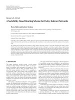
6. CELL-CYCLE PROGRESSION CONTROL
MODEL WITH RANDOM DELAYS AND
POSITIVE FEEDBACK
Our model can exhibit a pacemaker activity, initiating one-
cell division cycle after the previous one has finished with-
0 30 60 90 120 150 180
Time steps
F 0
2
T 0
2
v 0
2
w
1
0
2
x
1
0
2
y
1
0
2
z 0

2
State variables
(a) Due to the positive feedback from z to T, a new cycle is
started right after the previous one has finished, without the
need of a new F activator signal. This behavior is typical of
the embryonic cell-cycle, which depends on positive feedback
loops to maintain undamped oscillations with the correct tim-
ing
510 540 570 600 630 660 690
Time steps
F 0
2
T 0
2
v 0
2
w
1
0
2
x
1
0
2
y
1
0
2
z 0
2

State variables
(b) The second cycle in this figure is somewhat weakened (by
the effect of noise and random delays), but the positive feed-
back gets to overcome this (without the need of F activation)
and the system recovers its normal cyclical activity
Figure 8: PGN cell-cycle progression control model with positive
feedback from gene z to the trigger gene T (a
k
zT
= 7, k = 5+t
d
), 1%
of noise and only one initial activator pulse F
= 2att =−1, −2.
out the requirement of external stimuli, if we include positive
feedback in it. This oscillatory behavior is observed in nature
during proliferation of embryonic cells [4]. For our model to
present this oscillatory behavior, it suffices to include a pos-
itive feedback signal from gene z—last layer—to the trigger
gene T. The system is exactly the same as the previous ran-
dom delay PGN model, except for an additional weight dif-
ferent of zero: a
k
zT
= 7(wherek = 5+t
d
).
6.1. Experimental results
In the simulation of Figure 8, the system is initially driven by
a single pulse of F

= 2att =−1, −2. As in the embryonic cell
cycle, the positive feedback loop induces a pacemaker activity
10 EURASIP Journal on Bioinformatics and Systems Biology
where all cycles are completed normally with the correct tim-
ing for all the different phases. A new cycle starts right after
the completion of the previous one without the need of any
activator signal F. Figure 8(b) shows that when a signal wave
is weakened by the combined effect of noise and random de-
lays, the positive feedback (without the need of any F activa-
tion) is sufficient to overcome this signal failure, putting the
system back into a normal-amplitude cyclical activity. These
simulations show the flexibility of our PGN model to repre-
sent different types of dynamical behavior, including the em-
bryonic cell-cycle, that is induced by positive feedback loops.
7. DISCUSSION
We designed a PGN hypothetical model for control of cell-
cycle progression, inspired on qualitative description of well-
known biological phenomena: the cell cycle is a sequence
of events triggered by a control signal that propagates as a
wave; there are signal integrating subsystems and (positive
and negative) feedback loops; parallel replicated structures
make the cell-cycle control fault tolerant. Furthermore, im-
portant real-world nonbiological control systems usually are
designed to be stable, robust, fault tolerant and admit small
probabilistic parameter fluctuations.
Our model’s parameters were adjusted guided by the ex-
pected behavior of the system and exhaustive simulation.
This modeling effort had no intention of representing details
of molecular mechanisms such as kinetics and thermody-
namics of protein interactions, functioning of the transcrip-

tion machinery, microRNA, and transcription factors regu-
lation, but their concerted effects on the control of gene ex-
pression [13].
Our cell-cycle progression control model was able to rep-
resent some behavioral properties of the real biological sys-
tem, such as: (i) sequential waves of gene expression; (ii) sta-
bility in the presence of variable excitation; (iii) robustness
under noisy parameters: (iii-i) prediction by an almost de-
terministic stochastic rule; (iii-ii) stochastic choice of an al-
most deterministic stochastic prediction rule (random de-
lays), and (iv) auto stimulation by means of positive feed-
back.
The presence of numerous negative feedback loops in the
model provide stability and robustness. They warrant that,
under multiple noisy perturbation patterns, the system is
able to automatically correct external stimuli that could de-
stroy the cell. This kind of mechanisms has commonly been
found in nature. Particularly, we think that the robustness of
Li’s yeast cell-cycle model [3] would be improved by addition
of critical negative feedback loops, that we suspect should ex-
ist in the biological system. The inclusion of positive feed-
back can make our model capable of exhibiting a pacemaker
activity, like the one observed in embryonic cells. The par al-
lel structure of the system architecture represents biological
redundancy, which increases system fault tolerance.
Our discrete stochastic model qualitatively reproduces
the behavior of both Li et al. [3] and Pomerening et al. [4]
models, exhibiting remarkable robustness under noise and
parameters’ random variation. The natural follow up of this
research is to infer the PGN model from available dynam-

ical data of cell-cycle progression, analogously to what we
have done for the regulatory system of the malaria parasite
[5, 6]. We anticipate that, very likely, analysis of these dy-
namical data will uncover unknown negative feedback loops
in cell-cycle control mechanisms.
ACKNOWLEDGMENTS
This work was partially supported by Grants 99/07390-
0, 01/14115-7, 03/02717-8, and 05/00587-5 from FAPESP,
Brazil, and by Grant 1 D43 TW07015-01 from The National
Institutes of Health, USA.
REFERENCES
[1] A. Murray and T. Hunt, The Cell Cycle, Oxford University
Press, New York, NY, USA, 1993.
[2]B.Alberts,A.Johnson,J.Lewis,M.Raff,K.Roberts,andP.
Walter, Molecular Biology of the Cell, Garland Science, New
York, NY, USA, 4th edition, 2002.
[3] F. Li, T. Long, Y. Lu, Q. Ouyang, and C. Tang, “The yeast cell-
cycle network is robustly designed,” Proceedings of the National
Academy of Sciences of the United States of America, vol. 101,
no. 14, pp. 4781–4786, 2004.
[4] J. R. Pomerening, S. Y. Kim, and J. E. Ferrell Jr., “Systems-level
dissection of the cell-cycle oscillator: bypassing positive feed-
back produces damped oscillations,” Cell, vol. 122, no. 4, pp.
565–578, 2005.
[5] J.Barrera,R.M.CesarJr.,D.C.MartinsJr.,etal.,“Anewan-
notation tool for malaria based on inference of probabilistic
genetic networks,” in Proceedings of the 5th International Con-
ference for the Critical Assessment of Microarray Data Analy-
sis (CAMDA ’04), pp. 36–40, Durham, NC, USA, November
2004.

[6] J. Barrera, R. M. Cesar Jr., D. C. Martins Jr., et al., “Construct-
ing probabilistic genetic networks of plasmodium falciparum
from dynamical expression signals of the intraerythrocytic de-
velopement cycle,” in Methods of Microarray Data Analysis V,
chapter 2, Springer, New York, NY, USA, 2007.
[7] N.W.Trepode,H.A.Armelin,M.Bittner,J.Barrera,M.D.
Gubitoso, and R. F. Hashimoto, “Modeling cell-cycle regula-
tion by discrete dynamical systems,” in Proceedings of IEEE
Workshop on Genomic Signal Processing and Statistics (GEN-
SIPS ’05), Newport, RI, USA, May 2005.
[8] S.A.Kauffman, The Origins of Order, Oxford University Press,
New York, NY, USA, 1993.
[9] N. Friedman, M. Linial, I. Nachman, and D. Pe’er, “Using
Bayesian networks to analyze expression data,” Journal of Com-
putational Biology, vol. 7, no. 3-4, pp. 601–620, 2000.
[10] H. De Jong, “Modeling and simulation of genetic regulatory
systems: a literature review,” Journal of Computational Biology,
vol. 9, no. 1, pp. 67–103, 2002.
[11] I. Shmulevich, E. R. Dougherty, S. Kim, and W. Zhang, “Prob-
abilistic Boolean networks: a rule-based uncertainty model for
gene regulatory networks,” Bioinformatics,vol.18,no.2,pp.
261–274, 2002.
[12] J. Goutsias and S. Kim, “A nonlinear discrete dynamical model
for transcriptional regulation: construction and properties,”
Biophysical Journal, vol. 86, no. 4, pp. 1922–1945, 2004.
[13] S. Bornholdt, “Less is more in modeling large genetic net-
works,” Science, vol. 310, no. 5747, pp. 449–451, 2005.
Nestor Walter Trepode et al. 11
[14] P. T. Spellman, G. Sherlock, M. Q. Zhang, et al., “Comprehen-
sive identification of cell cycle-regulated genes of the yeast Sac-

charomyces cerevisiae by microarray hybridization,” Molecular
Biology of the Cell, vol. 9, no. 12, pp. 3273–3297, 1998.
[15] J. J. Tyson, K. Chen, and B. Novak, “Network dynamics and
cell physiology,” Nature Reviews Molecular Cell Biology, vol. 2,
no. 12, pp. 908–916, 2001.
[16] K. C. Chen, L. Calzone, A. Csikasz-Nagy, F. R. Cross, B. No-
vak,andJ.J.Tyson,“Integrativeanalysisofcellcyclecontrol
in budding yeast,” Molecular Biology of the Cell, vol. 15, no. 8,
pp. 3841–3862, 2004.
[17] H. A. Armelin, J. Barrera, E. R. Dougherty, et al., “Simulator
for gene expression networks,” in Microarrays: Optical Tech-
nologies and Informatic s, vol. 4266 of Proceedings of SPIE,pp.
248–259, San Jose, Calif, USA, January 2001.
[18] />∼walter/pgn cell cycle/ycc
info.pdf.
[19] />∼walter/pgn cell cycle/pgn
ccm add info.pdf.
[20] />∼walter/pgn cell cycle/pgn
ccmrd add info.pdf.