Báo cáo hóa học: " Research Article Comparison of Gene Regulatory Networks via Steady-State Trajectories" pdf

Hindawi Publishing Corporation
EURASIP Journal on Bioinformatics and Systems Biology
Volume 2007, Article ID 82702, 11 pages
doi:10.1155/2007/82702

Research Article
Comparison of Gene Regulatory Networks via
Steady-State Trajectories
Marcel Brun,1 Seungchan Kim,1, 2 Woonjung Choi,3 and Edward R. Dougherty1, 4, 5
1 Computational

Biology Division, Translational Genomics Research Institute, Phoenix, AZ 85004, USA
of Computing and Informatics, Ira A. Fulton School of Engineering, Arizona State University, Tempe, AZ 85287, USA
3 Department of Mathematics and Statistics, College of Liberal Arts and Sciences, Arizona State University, Tempe, AZ 85287, USA
4 Department of Electrical and Computer Engineering, Texas A&M University, College Station, TX 77843, USA
5 Cancer Genomics Laboratory, Department of Pathology, University of Texas M.D. Anderson Cancer Center, Houston,
TX 77030, USA
2 School

Received 31 July 2006; Accepted 24 February 2007
Recommended by Ahmed H. Tewfik
The modeling of genetic regulatory networks is becoming increasingly widespread in the study of biological systems. In the abstract, one would prefer quantitatively comprehensive models, such as a differential-equation model, to coarse models; however,
in practice, detailed models require more accurate measurements for inference and more computational power to analyze than
coarse-scale models. It is crucial to address the issue of model complexity in the framework of a basic scientific paradigm: the model
should be of minimal complexity to provide the necessary predictive power. Addressing this issue requires a metric by which to
compare networks. This paper proposes the use of a classical measure of difference between amplitude distributions for periodic
signals to compare two networks according to the differences of their trajectories in the steady state. The metric is applicable to
networks with both continuous and discrete values for both time and state, and it possesses the critical property that it allows
the comparison of networks of different natures. We demonstrate application of the metric by comparing a continuous-valued
reference network against simplified versions obtained via quantization.
Copyright © 2007 Marcel Brun et al. This is an open access article distributed under the Creative Commons Attribution License,

which permits unrestricted use, distribution, and reproduction in any medium, provided the original work is properly cited.

1.

INTRODUCTION

The modeling of genetic regulatory networks (GRNs) is becoming increasingly widespread for gaining insight into the
underlying processes of living systems. The computational
biology literature abounds in various network modeling approaches, all of which have particular goals, along with their
strengths and weaknesses [1, 2]. They may be deterministic
or stochastic. Network models have been studied to gain insight into various cellular properties, such as cellular state
dynamics and transcriptional regulation [3–8], and to derive
intervention strategies based on state-space dynamics [9, 10].
Complexity is a critical issue in the synthesis, analysis,
and application of GRNs. In principle, one would prefer
the construction and analysis of a quantitatively comprehensive model such as a differential equation-based model to a
coarsely quantized discrete model; however, in practice, the
situation does not always suffice to support such a model.
Quantitatively detailed (fine-scale) models require signifi-

cantly more complex mathematics and computational power
for analysis and more accurate measurements for inference
than coarse-scale models. The network complexity issue has
similarities with the issue of classifier complexity [11]. One
must decide whether to use a fine-scale or coarse-scale model
[12]. The issue should be addressed in the framework of the
standard engineering paradigm: the model should be of minimal complexity to solve the problem at hand.
To quantify network approximation and reduction, one
would like a metric to compare networks. For instance, it
may be beneficial for computational or inferential purposes

to approximate a system by a discrete model instead of a continuous model. The goodness of the approximation is measured by a metric and the precise formulation of the properties will depend on the chosen metric.
Comparison of GRN models needs to be based on salient
aspects of the models. One study used the L1 norm between
the steady-state distributions of different networks in the
context of the reduction of probabilistic Boolean networks


2

EURASIP Journal on Bioinformatics and Systems Biology

[13]. Another study compared networks based on their
topologies, that is, connectivity graphs [14]. This method
suffers from the fact that networks with the same topology
may possess very different dynamic behaviors. A third study
involved a comprehensive comparison of continuous models based on their inferential power, prediction power, robustness, and consistency in the framework of simulations,
where a network is used to generate gene expression data,
which is then used to reconstruct the network [15]. A key
drawback of most approaches is that the comparison is applicable only to networks with similar representations; it is
difficult to compare networks of different natures, for instance, a differential-equation model to a Boolean model. A
salient property of the metric proposed in this study is that it
can compare networks of different natures in both value and
time.
We propose a metric to compare deterministic GRNs via
their steady-state behaviors. This is a reasonable approach
because in the absence of external intervention, a cell operates mainly in its steady state, which characterizes its phenotype, that is, cell cycle, disease, cell differentiation, and
so forth. [16–19]. A cell’s phenotypic status is maintained
through a variety of regulatory mechanisms. Disruption of
this tight steady-state regulation may lead to an abnormal
cellular status, for example, cancer. Studying steady-state behavior of a cellular system and its disruption can provide significant insight into cellular regulatory mechanisms underlying disease development.

We first introduce a metric to compare GRNs based on
their steady-state behaviors, discuss its characteristics, and
treat the empirical estimation of the metric. Then we provide
a detailed application to quantization utilizing the mathematical framework of reference and projected networks. We
close with some remarks on the efficacy of the proposed
metric.
2.

METRIC BETWEEN NETWORKS

In this section, we construct the distance metric between networks using a bottom-up approach. Following a description
of how trajectories are decomposed into their transient and
steady-state parts, we define a metric between two periodic
or constant functions and then extend this definition to a
more general family of functions that can be decomposed between transient and steady-state parts.
2.1. Steady-state trajectory
Given the understanding that biological networks exhibit
steady-state behavior, we confine ourselves to networks exhibiting steady-state behavior. Moreover, since a cell uses nutrients such as amino acids and nucleotides in cytoplasm to
synthesize various molecular components, that is, RNAs and
proteins [18], and since there are only limited supplies of nutrients available, the amount of molecules present in a cell
is bounded. Thus, the existence of steady-state behavior implies that each individual gene trajectory can be modeled as a

bounded function f (t) that can be decomposed into a transient trajectory plus a steady-state trajectory:
f (t) = ftran (t) + fss (t),

(1)

where limt→∞ ftran (t) = 0 and fss (t) is either a periodic function or a constant function.
The limit condition on the transient part of the trajectory
indicates that for large values of t, the trajectory is very close

to its steady-state part. This can be expressed in the following
manner: for any > 0, there exists a time tss such that | f (t) −
fss (t)| < for t > tss . This property is useful to identify fss (t)
from simulated data by finding an instant tss such that f (t) is
almost periodical or constant for t > tss .
A deterministic gene regulatory network, whether it is
represented by a set of differential equations or state transition equations, produces different dynamic behaviors, depending on the starting point. If ψ is a network with N genes
and x0 is an initial state, then its trajectory,
(1)
(N)
f(ψ,x0 ) (t) = f(ψ,x0 ) (t), . . . , f(ψ,x0 ) (t) ,

(2)

(i)
where f(ψ,x0 ) (t) is a trajectory for an individual gene (denoted
by f (i) (t) or f (t) where there is no ambiguity) generated by
the dynamic behavior of the network ψ when starting at x0 .
For a differential-equation model, the trajectory f(ψ,x0 ) (t) can
be obtained as a solution of a system of differential equations;
for a discrete model, it can be obtained by iterating the system’s transition equations. Trajectories may be continuoustime functions or discrete-time functions, depending on the
model.
The decomposition of (1) applies to f(ψ,x0 ) (t) via its ap(i)
plication to the individual trajectories f(ψ,x0 ) (t). In the case
of discrete-valued networks (with bounded values), the system must enter an attractor cycle or an attractor state at some
time point tss . In the first case f(ψ,x0 ),ss (t) is periodical, and in
the second case it is constant. In both cases, f(ψ,x0 ),tran (t) = 0
for t ≥ tss .

2.2.

Distance based on the amplitude
cumulative distribution

Different metrics have been proposed to compare two realvalued trajectories f (t) and g(t), including the correlation
f , g , the cross-correlation Γ f ,g (τ), the cross-spectral density p f ,g (ω), the difference between their amplitude cumulative distributions F(x) = p f (x) and G(x) = pg (x), and the
difference between their statistical moments [20]. Each has
its benefits and drawbacks depending on one’s purpose. In
this paper, we propose using the difference between the amplitude cumulative distributions of the steady-state trajectories.
Let fss (t) and gss (t) be two measurable functions that are
either periodical or constant, representing the steady-state
parts of two functions, f (t) and g(t), respectively. Our goal
is to define a metric (distance) between them by using the


Marcel Brun et al.

3

0.9

4

0.8

3

0.7

2

0.6
F(x)

1

5

x = f (t)

6

1

0.5

0

0.4

−1

0.3

−2

0.2

−3

0.1

−4

0

200

400

600

0

−4

800 1000 1200 1400 1600 1800 2000
t

−3

−2

−1

0

1

2

3

4

5

6

x
2∗ sin(t)
2∗ cos(2∗ t + 1)
2∗ sin(t) + 2∗ sin(2∗ t)

(a)

2∗ sin(t) + 2∗ sin(2∗ t) + 2
3 + 0∗ t
4 + 0∗ t

(b)

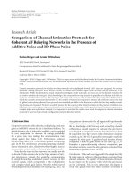
Figure 1: Example of (a) periodical and constant functions f (t) and (b) their amplitude cumulative distributions F(x).

amplitude cumulative distribution (ACD), which measures
the probability density of a function [20].
If fss (t) is periodic with period t p > 0, its cumulative densityfunction F(x) over R is defined by
F(x) = λ

M(x)

,
tp

(3)

where λ(A) isthe Lebesgue measure of the set A and
M(x) = ts ≤ t < te | fss (t) ≤ x ,

(4)

where te = ts + t p , for any point ts .
If fss is constant, given by fss (t) = a for any t, then we
define F(x) as a unit step function located at x = a. Figure 1
shows an example of some periodical functions and their amplitude cumulative distributions.
Given two steady-state trajectories, fss (t) and gss (t), and
their respective amplitude cumulative distributions, F(x)
and G(x), we define the distance between fss and gss as the
distance between the distributions
dss fss , gss = F − G

(5)

for some suitable norm · . Examples of norms include L∞ ,
defined by the supremum of their differences,
dL∞ ( f , g) = sup

0≤x≤∞

F(x) − G(x) ,

(6)

and L1 defined by the area of the absolute value of their difference,
dL1 ( f , g) =

0≤x<∞

F(x) − G(x) dx.

(7)

In both cases, we apply the biological constraint that the amplitudes are nonnegative.
The L1 norm is well suited to the steady-state behavior because in the case of constant functions f (t) = a and
g(t) = b, their distributions are unit steps functions at x = a
and x = b, respectively, so that dL1 ( f , g) = |a − b|, the distance, in amplitude, between the two functions. Hence, we
can interpret the distance dL1 ( f , g) as an extension of the distance, in amplitude, between two constant signals, to the general case of periodic functions, taking into consideration the
differences in their shapes.
2.3.

Network metric

Once a distance between their steady-state trajectories is defined, we can extend this distance to two trajectories f (t) and
g(t) by
dtr ( f , g) = dss fss , gss ,

(8)

where dss is defined by (5).
The next step is to define the distance between two multivariate trajectories f(t) and g(t) by
dtr (f, g) =

1
N

N

dtr f (i) , g (i) ,

(9)

i=1

where f (i) (t) and g (i) (t) are the component trajectories of
f(t) and g(t), respectively. Owing to the manner in which a
norm is used to define dss , in conjunction with the manner
in which dtr is constructed from dss , the triangle inequality
dtr (f, h) ≤ dtr (f, g) + dtr (g, h)

(10)


4

EURASIP Journal on Bioinformatics and Systems Biology

holds, and dtr is a metric.
The last step is to define the metric between two networks
as the expected distance between the trajectories over all possible initial states. For networks ψ1 and ψ2 , we define
d ψ1 , ψ2 = ES dtr f(ψ1 ,x0 ) , f(ψ2 ,x0 ) ,

(11)

where the expectation is taken with respect to the space S of
initial states.
The use of a metric, in particular, the triangle inequality,
is essential for the problem of estimating complex networks
by using simpler models. This is akin to the pattern recognition problem of estimating a complex classifier via a constrained classifier to mitigate the data requirement. In this
situation, there is a complex model that represents a broad
family of networks and a simpler model that represents a
smaller class of networks. Given a reference network from the
complex model and a sampled trajectory from it, we want to
estimate the optimal constrained network. We can identify
the optimal constrained network, that is, projected network,
as the one that best approximates the complex one, and the
goal of the inference process should be to obtain a network
close to the optimal constrained network. Let ψ be a reference
network (e.g., a continuous-valued ODE-based network), let
P(ψ) be the optimal constrained network (e.g., a discretevalued network), and let ω be an estimator of P(ψ) estimated
from data sampled from ψ. Then
d(ω, ψ) ≤ d ω, P(ψ) + d P(ψ), ψ ,

(12)

x

t0

t1

t2

This structure is analogous to the classical constrained regression problem, where constraints are used to facilitate better inference via reduction of the estimation error (so long as
this reduction exceeds the projection error) [11]. In the case
of networks, the constraint problem becomes one of finding
a projection mapping for models representing biological processes for which the loss defined by d(P(ψ), ψ) may be maintained within manageable bounds so that with good inference techniques, the estimation error defined by d(ω, P(ψ))
will be minimized.
2.4. Estimation of the amplitude
cumulative distribution
The amplitude cumulative distribution of a trajectory can be
estimated by simulating the trajectory and then estimating
the ACD from the trajectory. Assuming that the steady-state

ti+1
mi = f

ti+2
ti + ti+1
2

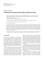
Figure 2: Example of determination of values mi .

trajectory fss (t) is periodic with period t p , we can analyze
fss (t) between two points, ts and te = ts + t p . For a continuous function fss (t), we assume that any amplitude value x
is visited only a finite number of times by fss (t) in a period
ts ≤ t < te . In accordance with (3), we define the cumulative
distribution
F(x) =

λ ts ≤ t ≤ te | fss (t) ≤ x
tp

.

(13)

To calculate F(x) from a sampled trajectory, for each value x,
let Sx be the set of points where fss (t) = x:
Sx = ts ≤ t ≤ te | fss (t) = x ∪ ts , te .

(14)

The set Sx is finite. Let n = |Sx | denote the number of elements t0 , . . . , tn−1 . These can be sorted so that ts = t0 <
t1 < t2 < · · · < tn−1 = te . Now we define the set mi ,
i = 0, . . . , n − 2, of intermediate values between two consecutive points where fss (t) crosses x (see Figure 2) by
mi = fss

where the following distances have natural interpretations:
(i) d(ω, ψ) is the overall distance and quantifies the approximation of the reference network by the estimated
optimal constrained network;
(ii) d(ω, P(ψ)) is the estimation distance for the constrained network and quantifies the inference of the
optimal constrained network;
(iii) d(P(ψ), ψ) is the projection distance and quantifies how
well the optimal constrained network approximates
the reference network.

ti

ti + ti+1
.
2

(15)

Let Ix be a set of the indices of points ti such that the
function f (t) is below x in the interval [ti , ti+1 ],
Ix = 0 ≤ i ≤ n − 2 | mi ≤ x .

(16)

Finally, the cumulative distribution F(x), defined by the measure of the set {ts ≤ t ≤ te | f (t) ≤ x}, can be computed as
the sum of the lengths of the intervals where f (t) ≤ x:
F(x) =

i∈Ix

ti+1 − ti
.
tp

(17)

The estimation of F(x) from a finite set {a1 , . . . , am } representing the function f (t) at points t1 , . . . , tm reduces to estimating the values in (17):
F(x) =

1 ≤ i ≤ m | ai ≤ x
m

(18)

at the points ai , i = 1, . . . , m.

In the case of computing the distance between two functions f (t) and g(t), where the only information available
consists of two samples, {a1 , . . . , am } and {b1 , . . . , br }, for f
and g, respectively, both cumulative distributions F(x) and
G(x) need only be defined at the points in the set
S = a1 , . . . , am ∪ b1 , . . . , br .

(19)


Marcel Brun et al.

5

p1 (t)

r1 (t)
Translation

r3 (t)
Cis-regulation

Transcription

r2 (t)
Translation
p2 (t)

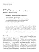
Figure 3: Block diagram of a model for transcriptional regulation.

In this case, if we sort the set S so that 0 = s0 < s2 < · · · <

sk = T (with T being the upper limit for the amplitude values, and k ≤ r + m), then (6) can be approximated by
dL∞ ( f , g) = max F si − G si

(20)

0≤i≤k

and (7) can be approximated by
si+1 − si F si − G si

dL1 ( f , g) =

.

(21)

0≤i≤k−1

3.

APPLICATION TO QUANTIZATION

To illustrate application of the network metric, we will analyze how different degrees of quantization affect model accuracy. Quantization is an important issue in network modeling because it is imperative to balance the desire for fine
description against the need for reduced complexity for both
inference and computation. Since it is difficult, if not impossible, to directly evaluate the goodness of a model against a
real biological system, we will study the problem using a standard engineering approach. First, an in numero reference network model or system is formulated. Then, a second network
model with a different level of abstraction is introduced to
approximate the reference system. The objective is to investigate how different levels of abstraction, quantization levels in
this study, impact the accuracy of the model prediction. The
first model is called the reference model. From it, reference

networks will be instantiated with appropriate sets of model
parameters. The model will be continuous-valued to approximate the reference system at its fullest closeness. The second
model is called a projected model, and projected networks will
be instantiated from it. This model will be a discrete-valued
model at a given different level of quantization.
The ability of a projected network, an instance of the
projected model, to approximate a reference network, an instance of the reference model, can be evaluated by comparing
the trajectories generated from each network with different
initial states and computing the distances between the networks as given by (11).

3.1.

Reference model

The origin of our reference model is a differential-equation
model that quantitatively represents transcription, translation, cis-regulation and chemical reactions [7, 15, 21]. Specifically, we consider a differential-equation model that approximates the process of transcription and translation for
a set of genes and their associated proteins (as illustrated in
Figure 3) [7].The model comprises the following differential
equations:
d pi (t)
= λi ri t − τ p,i − γi pi (t), i ∈ G,
dt
dri (t)
= κi ci t − τr,i − βi ri (t), i ∈ G,
dt
ci (t) = φi p j t − τc, j , j ∈ Ri , i ∈ G,

(22)

where ri and pi are the concentrations of mRNA and proteins induced by gene i, respectively, ci (t) is the fraction of

DNA fragments committed to transcription of gene i, κi is the
transcription rate of gene i, and τ p,i , τr,i , and τc,i are the time
delays for each process to start when the conditions are given.
The most general form for the function φi is a real-valued
(usually nonlinear) function with domain in R|Ri | and range
in R, φi : R|Ri | → R. The functions are defined by the equations
φi p j , j ∈ Ri = 1 −

ρ p j , Si j , θi j
j ∈Ri+

×

ρ p j , Si j , θi j ,

(23)

j ∈Ri−

ρ(p, S, θ) =

1
,
(1 + θ p)S

where the parameters θ are the affinity constants and the parameters Si j are the distinct sites for gene i where promoter
j can bind. The functions depend on the discrete parameter
Si j , the number of binding sites for protein j on gene i, and
θi j , the affinity constant between gene i and protein j.
A discrete-time model results from the preceding

continuous-time model by discretizing the time t on intervals nδt, and the assumption that the fraction of DNA


6

EURASIP Journal on Bioinformatics and Systems Biology
Table 1: Parameter values used in simulations.
Parameter
Affinity constant

Value
θ = 108 M−1

Parameter
Number of binding sites

mRNA and protein half-life

ρ = 1200 s
π = 3600 s

Transcription rates

Translation rate

λ = 0.20 s−1

Value
S=1
κ1 = 0.001 pMs−1

κ2 = κ3 = κ4 = 0.05 pMs−1

Time delays

Transcription

Input substrate
concentration

1

1
2

2

3

3

3

4

4
Translation

Projected model

The next step is to reduce the reference network model to

a projected network model. This is accomplished by applying constraints in the reference model. The application of
constraints modifies the original model, thereby obtaining
a simpler one. We focus on quantization of the gene expression levels (which are continuous-valued in the reference model) via uniform quantization, which is defined by
a finite or denumerable set L of intervals, L1 = [0, Δx ),
L2 = [Δx , 2Δx ), . . . , Li = [(i − 1)Δx , iΔx ), . . . , and a mapping ΠL : R → R such that Π(x) = ai for some collection of
points ai ∈ Li .
The equations for ri , pi , and ci (24) are replaced by

1

2

3.2.

τr = 2000 s
τc = 200 s
τ p = 2400 s

4
Cis-regulation

mRNA
Protein
Gene

r i (n) = Π e−βi δt r i (n − 1) + κi s βi , δt ci n − nr,i − 1 ,
(27)

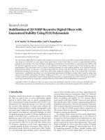
Figure 4: Example of a tRS of a hypothetical metabolic pathway
that consists of four genes. In this figure,

denotes an activator,
whereas, denotes a repressor.

fragments committed to transcription and concentration of
mRNA remains constant in the time interval [t − δt, t) [7].
In place of the differential equations for ri , pi , and ci , at time
t = nδt, we have the equations
ri (n) = e−βi δt ri (n − 1) + κi s(βi , δt)ci n − nr,i − 1 ,
pi (n) = e−γi δt pi (n − 1) + λi s λi , δt ri n − n p,i − 1 ,
ci (n) = φi p j n − nc, j , j ∈ Ri ,

(25)

This model, which will serve as our reference model, is called
a (discrete) transcriptional regulatory system (tRS).
We generate networks using this model and a fixed set θ
of parameters. We call these networks reference networks. A
reference network is identified by its set θ of parameters,
θ = α1 , β1 , λ1 , γ1 , κ1 , τ p,1 , τr,1 , τc,1 , φ1 , R1 , . . . , αN ,
βN , λN , γN , κN , τ p,N , τr,N , τc,N , φN , RN .

i ∈ G.

(29)

Issues to be investigated include (1) how different quantization techniques (specification of the partition L) affect
the quality of the model; (2) which quantization technique
(mapping Π) is the best for the model; and (3) the similarity
of the attractors of the dynamical system defined by (27) and
(28) to the steady state of the original system, as a function

of Δx . We consider the first issue.
3.3.

i ∈ G,

1 − e−xy
.
x

ci (n) = φi p j n − nc, j , j ∈ Ri ,

A hypothetical metabolic pathway

(24)

where nr,i = τr,i /δt, n p,i = τ p,i /δt, nc, j = τc, j /δt, and
s(x, y) =

pi (n) = Π e−γi δt pi (n − 1) + λi s λi , δt r i n − n p,i − 1 ,
(28)

(26)

To illustrate the proposed metric in the framework of the
reference and projected models, we compare two networks
based on a hypothetical metabolic pathway. We first briefly
describe the hypothetical metabolic pathway with necessary
biochemical parameters to set up a reference system. Then,
the simulation study shows the impacts of various quantization levels in both time and trajectory based on the proposed
metric.

We consider a gene regulatory network consisting of four
genes. A graphical representation of the system is depicted
in Figure 4, where
denotes an activator and denotes a
repressor. We assume that the GRN regulates a hypothetical
pathway, which metabolizes an input substrate to an output
product. This is done by means of enzymes whose transcriptional control is regulated by the protein produced from gene
3. Moreover, we assume that the effect of a higher input substrate concentration is to increase the transcription rate κ1 ,


Marcel Brun et al.

7
Gene 1

6

Gene 2

50

5

40

4
30
3
20
2

10

1

0

0
Initial

Final

10000 seconds

Initial

10000 seconds

10000 seconds

Quant = 0
Q = 0.001, S = 0.06, Sn = 0
Q = 0.01, S = 0.5, Sn = 0
Q = 0.1, S = 1.7, Sn = 0

10000 seconds

Quant = 0
Q = 0.001, S = 0.65, Sn = 0.82
Q = 0.01, S = 6.65, Sn = 0
Q = 0.1, S = 49.5, Sn = 0

(a)

(b)

Gene 4

Gene 3

120

Final

200

100
150
80
100

60
40

50
20
0

0
Initial

Final

10000 seconds

10000 seconds

Quant = 0
Q = 0.001, S = 0.63, Sn = 0.13
Q = 0.01, S = 4.34, Sn = 13
Q = 0.1, S = 111.66, Sn = 13
(c)

Initial

Final

10000 seconds

10000 seconds

Quant = 0
Q = 0.001, S = 9.76, Sn = 0.07
Q = 0.01, S = 52.18, Sn = 0.89
Q = 0.1, S = 58.96, Sn = 0.89
(d)

Figure 5: Example of trajectories from the first simulation of 4-gene network. Each figure shows the trajectory for one of the four genes, for
several values of the level quantization Δx , represented by the lines Q = 0, Q = 0.001, Q = 0.01 and Q = 0.1 (Q = 0 represents the original
network without quantization). The values S displayed in the graphs shows the distance computed between the trajectory and the one with
Q=0. The vertical axis shows the concentration levels x in pM. The horizontal axis shows the time t in seconds.

whereas the effect of a lower substrate concentration is to reduce κ1 . Unless otherwise specified, the parameters are assumed to be gene-independent. These parameters are summarized in Table 1.

We assume that each cis-regulator is controlled by one
module with four binding sites, and set S = 4, θ = 108 M−1 ,
κ2 = κ3 = κ4 = 0.05 pMs−1 , and λ = 0.05 s−1 . The value of
the affinity constant θ corresponds to a binding free energy


8

EURASIP Journal on Bioinformatics and Systems Biology
Iter. 1, gene 2

Iter. 1, gene 1
1

0.8

0.8

0.6

0.6
F(x)

F(x)

1

0.4

0.4

0.2

0.2

0

0

0.5

1
x

1.5

0

2

0

Quant = 0
Q = 0.0001, S = 0.06, Sn = 0
Q = 0.01, S = 0.5, Sn = 0
Q = 0.1, S = 1.7, Sn = 0

10

20

30
x

40

50

60

Quant = 0
Q = 0.001, S = 0.65, Sn = 0.82
Q = 0.01, S = 6.65, Sn = 0
Q = 0.1, S = 49.5, Sn = 0

(a)

(b)

Iter. 1, gene 3

Iter. 1, gene 4

0.8

0.8

0.6

0.6
F(x)

1

F(x)

1

0.4

0.4

0.2

0.2

0

0

50

100

150

0

0

50

100
x

x
Quant = 0
Q = 0.001, S = 0.63, Sn = 0.13
Q = 0.01, S = 4.34, Sn = 1.3
Q = 0.1, S = 111.66, Sn = 1.3

150

200

Quant = 0
Q = 0.001, S = 9.76, Sn = 0.07
Q = 0.01, S = 52.18, Sn = 0.89
Q = 0.1, S = 58.96, Sn = 0.89

(c)

(d)

Figure 6: Example of estimated cumulative density function (CDF) from the first simulation of 4-gene network, computed from the trajectories in Figure 5. Each figure shows the CDF for one of the four genes, for several values of the level quantization Δx , represented by the lines
Q = 0, Q = 0.001, Q = 0.01, and Q = 0.1 (Q = 0 represents the original network without quantization). The value S displayed in the graphs
show the distance computed between the trajectory and the one with Q = 0. The vertical axis shows the cumulative distribution F(x). The

horizontal axis shows the concentration levels x in pM.

of ΔU = −11.35 kcal/mol at temperature T = 310.15◦ K (or
37◦ C). The values of the transcription rates κ2 , κ3 , and κ4 correspond to transcriptional machinery that, on the average,
produces one mRNA molecule every 8 seconds. This value
turns out to be typical for yeast cells [22]. We also assume
that on the average, the volume of each cell in C equals 4 pL
[18]. The translation rate λ is taken to be 10-fold larger than
the rate of 0.3/minute for translation initiation observed in
vitro using a semipurified rabbit reticulocyte system [23].

The degradation parameters β and γ are specified by
means of the mRNA and protein half-life parameters ρ and
π, respectively, which satisfy
1
e−βρ = ,
2

1
e−γπ = .
2

(30)

ln 2
.
π

(31)

In this case,
β=

ln 2
,
ρ

γ=


Marcel Brun et al.

9
80
70

120
100

60

80

50
60

40

40
20

0
3600
1800
600

30
20
300

120

δt

101
60

100
30

10

5
1

10−3

10−2

10−1

Δx

10
0

1

5

10

30

60 120

300 600

1800 3600

δt

Figure 7: Results for the first simulation: the vertical axis shows the
distance dL1 ( f(Δx ,δt ) , f(Δx =0,δt ) ) as function of quantization levels for
both the values (axis labeled “Δx ”) and the time (axis labeled “δt ”).

Δx = 0.1
Δx = 1

Δx = 0
Δx = 0.001

Δx = 0.01
(a)

3.4. Results and discussion
It is expected that the finer the quantization is (smaller values of Δx ), the more similar will be the projected networks
to the reference networks. This similarity should be reflected
by the trajectories as measured by the proposed metric. A
straightforward simulation consists of the design of a reference network, the design of a projected network (for some
value of Δx ), the generation of several trajectories for both
networks from randomly selected starting points, and the
computation of the average distance between trajectories, using (9) and (21). Each process is repeated for different time
intervals δt to study how the time intervals used in the simulation affect the analysis.
The firstsimulation is based on the same 4-gene model
presented in [7]. We use 6 different quantization levels,
Δx = 0, 0.001, 0.01, 0.1, 1, and 10, where Δx = 0 means
no quantization, and designates the reference network. For
each quantization level Δx and starting point x0 , we generate the simulated time series expression and compare it to
the time-series generated with Δx = 0 (the reference network), estimating the proposed metric using (21). The process is repeated using a total of 10 different time intervals,
δt = 1 second, 5 seconds, 10 seconds, 30 seconds, 1 minute,
2 minutes, 5 minutes, 10 minutes, 30 minutes, and 1 hour.
The simulation is repeated and the distances are averaged for
30 different starting points x0 .
Figures 5 and 6 show the trajectories and empirical cumulative density functions estimated from the simulated system as illustrated in the previous section. Several quantization levels are used in the simulation. The last graph in
Figure 5 shows the mRNA concentration for the forth gene,
over the 10 000 first seconds (transient) and over the last
10 000 seconds (steady-state). We can see that for quantizations 0 and 0.001, the steady-state solutions are periodic, and
for quantizations 0.001 and 0.1, the solutions are constant.
This is reflected by the associated plot of F(x) in Figure 6.

120

100
80
60
40
20
0
10−3

10−2

10−1
Δx

δt = 1
δt = 10
δt = 60

100

101

δt = 300
δt = 1800
(b)

Figure 8: Results for the first simulation: the vertical axis shows the
distance dL1 ( f(Δx ,δt ) , f(Δx =0,δt ) ) as function of quantization levels for
both the values (labeled “Δx ”) and the time (labeled “δt ”). Part (a)
shows the distance as a function of Δx for several values of δt . Part
(b) shows the distance as a function of δt for several values of Δx .

Figure 7 shows how strong quantization (high values of
Δx ) yields high distance, with the distance decreasing again
when the time interval (δt ) increases. The z-axis in the figure
represents the distance dL1 ( f(Δx ,δt ) , f(Δx =0,δt ) ).
In our second simulation, we use a different connectivity (all other kinetic parameters are unchanged), and we


10

EURASIP Journal on Bioinformatics and Systems Biology
40
35

40
35

30

30
25

25

20
15

20

10

15

5
0
3600
1800
600

10
300

120

δt

101
60

100
30

10

5
1

10−3

10−2

10−1

Δx

5
0

1

5

10

30

60 120

300 600

1800 3600

δt

Figure 9: Results for the second simulation: the vertical axis shows
the distance dL1 ( f(Δx ,δt ) , f(Δx =0,δt ) ) as function of quantization levels
for both the values (axis labeled “Dx”) and the time (axis labeled
“delta t”).

Δx = 0

Δx = 0.001
Δx = 0.01

Δx = 0.1
Δx = 1
(a)

again use 10 different time intervals, δt = 1 second, 5 seconds,
10 seconds, 30 seconds, 1 minute, 2 minutes, 5 minutes,
10 minutes, 30 minutes and 1 hour, and 6 different quantization levels, Δx = 0, 0.001, 0.01, 0.1, 1, and 10. (Δx = 0
meaning no quantization). The simulation is repeated and
the distances are averaged for 30 different starting points.
Analogous to the first simulation, Figure 9 shows how strong
quantization (high values of Δx ) yields high distance, which
decreases when the time interval (δt ) increases.
An important observation regarding Figures 8 and 10 is
that the error decreases as δt increases. This is due to the fact
that the coarser the amplitude quantization is, the more difficult it is for small time intervals to capture the dynamics of
slowly changing sequences.
4.

CONCLUSION

This study has proposed a metric to quantitatively compare
two networks and has demonstrated the utility of the metric via a simulation study involving different quantizations of
the reference network. A key property of the proposed metric
is that it allows comparison of networks of different natures.
It also takes into consideration differences in the steady-state
behavior and is invariant under time shifting and scaling.
The metric can be used for various purposes besides quantization issues. Possibilities include the generation of a projected network from a reference network by removing proteins from the equations and connectivity reduction by removing edges in the connectivity matrix.

The metric facilitates systematic study of the ability
of discrete dynamical models, such as Boolean networks,
to approximately represent more complex models, such as
differential-equation models. This can be particularly important in the framework of network inference, where the parameters for projected models can be inferred from the reference model, either analytically or via synthetic data generated via simulation of the reference model. Then, given the

40
35
30
25
20
15
10
5
0
10−3

10−2

10−1
Δx

δt = 1
δt = 10
δt = 60

100

101

δt = 300

δt = 1800
(b)

Figure 10: Results for the second simulation: the vertical axis shows
the distance dL1 ( f(Δx ,δt ) , f(Δx =0,δt ) ) as function of quantization levels
for both the values (labeled “Δx ”) and the time (labeled “δt ”). Part
(a) shows the distance as a function of Δx for several values of δt .
Part (b) shows the distance as a function of δt for several values of
Δx .

reference and projected models, the metric can be used to
determine the level of abstraction that provides the best inference; given the amount of observations available, this approach corresponds to classification-rule constraint for classifier inference in pattern recognition.


Marcel Brun et al.

11

NOMENCLATURE
Trajectory:
A function f (t)
Distance Function: The proposed distance between
networks
NOTATIONS
t:
ψ:
x0 :
f (t), g(t), h(t):
fss , gss :
fψ,xo (t):

ftran :
fss :
F(x), G(x), H(x):
dtr (·, ·):
dss (·, ·):
λ(A):
f(t):

Time
Network
Starting Point
Trajectories
Steady-State trajectories
Trajectory
Transient part of the trajectory
Steady-state part of the trajectory
Cumulative distribution functions
Distance between two trajectories
Distance between two periodic or constant
trajectories
Lebesgue measure of set A
Multivariate trajectory

ACKNOWLEDGMENTS
We would like to thank the National Science Foundation
(CCF-0514644) and the National Cancer Institute (R01 CA104620) for sponsoring in part this research.
REFERENCES
[1] H. De Jong, “Modeling and simulation of genetic regulatory
systems: a literature review,” Journal of Computational Biology,
vol. 9, no. 1, pp. 67–103, 2002.

[2] R. Srivastava, L. You, J. Summers, and J. Yin, “Stochastic vs.
deterministic modeling of intracellular viral kinetics,” Journal
of Theoretical Biology, vol. 218, no. 3, pp. 309–321, 2002.
[3] R. Albert and A.-L. Barab´ si, “Statistical mechanics of coma
plex networks,” Reviews of Modern Physics, vol. 74, no. 1, pp.
47–97, 2002.
[4] S. Kim, H. Li, E. R. Dougherty, et al., “Can Markov chain models mimic biological regulation?” Journal of Biological Systems,
vol. 10, no. 4, pp. 337–357, 2002.
[5] R. Albert and H. G. Othmer, “The topology of the regulatory
interactions predicts the expression pattern of the segment polarity genes in Drosophila melanogaster,” Journal of Theoretical
Biology, vol. 223, no. 1, pp. 1–18, 2003.
[6] S. Aburatani, K. Tashiro, C. J. Savoie, et al., “Discovery of
novel transcription control relationships with gene regulatory
networks generated from multiple-disruption full genome expression libraries,” DNA Research, vol. 10, no. 1, pp. 1–8, 2003.
[7] J. Goutsias and S. Kim, “A nonlinear discrete dynamical model
for transcriptional regulation: construction and properties,”
Biophysical Journal, vol. 86, no. 4, pp. 1922–1945, 2004.
[8] H. Li and M. Zhan, “Systematic intervention of transcription
for identifying network response to disease and cellular phenotypes,” Bioinformatics, vol. 22, no. 1, pp. 96–102, 2006.

[9] A. Datta, A. Choudhary, M. L. Bittner, and E. R. Dougherty,
“External control in Markovian genetic regulatory networks,”
Machine Learning, vol. 52, no. 1-2, pp. 169–191, 2003.
[10] A. Choudhary, A. Datta, M. L. Bittner, and E. R. Dougherty,
“Control in a family of boolean networks,” in IEEE International Workshop on Genomic Signal Processing and Statistics
(GENSIPS ’06), College Station, Tex, USA, May 2006.
[11] L. Devroye, L. Gyă r, and G. Lugosi, A Probabilistic Theory of
o
Pattern Recognition, Springer, New York, NY, USA, 1996.
[12] I. Ivanov and E. R. Dougherty, “Modeling genetic regulatory

networks: continuous or discrete?” Journal of Biological Systems, vol. 14, no. 2, pp. 219–229, 2006.
[13] I. Ivanov and E. R. Dougherty, “Reduction mappings between
probabilistic boolean networks,” EURASIP Journal on Applied
Signal Processing, vol. 2004, no. 1, pp. 125–131, 2004.
[14] S. Ott, S. Imoto, and S. Miyano, “Finding optimal models for
small gene networks,” in Proceedings of the Pacific Symposium
on Biocomputing (PSB ’04), pp. 557–567, Big Island, Hawaii,
USA, January 2004.
[15] L. F. Wessels, E. P. van Someren, and M. J. Reinders, “A comparison of genetic network models,” in Proceedings of the Pacific Symposium on Biocomputing (PSB ’01), pp. 508–519, Lihue, Hawaii, USA, January 2001.
[16] M. B. Elowitz, A. J. Levine, E. D. Siggia, and P. S. Swain,
“Stochastic gene expression in a single cell,” Science, vol. 297,
no. 5584, pp. 1183–1186, 2002.
[17] S. A. Kauffman, The Origins of Order: Self-Organization and
Selection in Evolution, Oxford University Press, New York, NY,
USA, 1993.
[18] B. Alberts, A. Johnson, J. Lewis, M. Raff, K. Roberts, and P.
Walter, Molecular Biology of the Cell, Garland Science, New
York, NY, USA, 4th edition, 2002.
[19] S. A. Kauffman, “Metabolic stability and epigenesis in randomly constructed genetic nets,” Journal of Theoretical Biology,
vol. 22, no. 3, pp. 437–467, 1969.
[20] P. A. Lynn, An Introduction to the Analysis and Processing of
Signals, John Wiley & Sons, New York, NY, USA, 1973.
[21] A. Arkin, J. Ross, and H. H. McAdams, “Stochastic kinetic
analysis of developmental pathway bifurcation in phage λinfected Escherichia coli cells,” Genetics, vol. 149, no. 4, pp.
1633–1648, 1998.
[22] V. Iyer and K. Struhl, “Absolute mRNA levels and transcriptional initiation rates in Saccharomyces cerevisiae,” Proceedings
of the National Academy of Sciences of the United States of America, vol. 93, no. 11, pp. 5208–5212, 1996.
[23] J. R. Lorsch and D. Herschlag, “Kinetic dissection of fundamental processes of eukaryotic translation initiation in vitro,”
EMBO Journal, vol. 18, no. 23, pp. 6705–6717, 1999.