Báo cáo hóa học: " Research Article A Low Delay and Fast Converging Improved Proportionate Algorithm for Sparse System Identification" potx

Hindawi Publishing Corporation
EURASIP Journal on Audio, Speech, and Music Processing
Volume 2007, Article ID 84376, 8 pages
doi:10.1155/2007/84376
Research Article
A Low Delay and Fast Converging Improved Proportionate
Algorithm for Sparse System Identification
Andy W. H. Khong,
1
Patrick A. Naylor,
1
and Jacob Benesty
2
1
Department of Electrical and Electronic Engineering, Imperial College London, Exhibition Road, London SW7 2AZ, UK
2
INRS-EMT, Universit
´
eduQu
´
ebec, Suite 6900, 800 de la Gaucheti
`
ere Ouest, Montr
´
eal, QC, Canada H5A 1K6
Received 4 July 2006; Revised 1 December 2006; Accepted 24 January 2007
Recommended by Kutluyil Dogancay
A sparse system identification algorithm for network echo cancellation is presented. This new approach exploits both the fast
convergence of the improved proportionate normalized least mean square (IPNLMS) algorithm and the efficient implementation
of the multidelay adaptive filtering (MDF) algorithm inheriting the beneficial properties of both. The proposed IPMDF algorithm
is evaluated using impulse responses with various degrees of sparseness. Simulation results are also presented for both speech

and white Gaussian noise input sequences. It has been shown that the IPMDF algorithm outperforms the MDF and IPNLMS
algorithms for both sparse and dispersive echo path impulse responses. Computational complexity of the proposed algorithm is
also discussed.
Copyright © 2007 Andy W. H. Khong et al. This is an open access article distributed under the Creative Commons Attribution
License, which permits unrestricted use, distribution, and reproduction in any medium, provided the original work is properly
cited.
1. INTRODUCTION
Research on network echo cancellation is increasingly im-
portant with the advent of voice over internet protocol
(VoIP). In such systems where traditional telephony equip-
ment is connected to the packet-switched network, the echo
path impulse response, which is typically of length 64–
128 milliseconds, exhibits an “active” region in the range of
8–12 milliseconds duration and consequently, the impulse
response is dominated by regions where magnitudes are close
to zero making the impulse response sparse. The “inactive”
region is due to the presence of bulk delay caused by network
propagation, encoding, and jitter buffer delays [1]. Other
applications for sparse system identification include wavelet
identification using marine seismic signals [2] and geophysi-
cal seismic applications [3, 4].
Classical adaptive algorithms with a uniform step-size
across all filter coefficients such as the normalized least mean
square (NLMS) algorithm have slow convergence in sparse
network echo cancellation applications. One of the first algo-
rithms which exploits the sparse nature of network impulse
responses is the proportionate normalized least mean square
(PNLMS) algorithm [5]whereeachfiltercoefficient is up-
dated with an independent step-size which is proportional
to the estimated filter coefficient. Subsequent improved ver-

sions such as the IPNLMS [6] and IIPNLMS [7] algorithms
were proposed, which achieve improved convergence by in-
troducing a controlled mixture of proportionate (PNLMS)
and nonproportionate (NLMS) adaptation. Consequently,
these algor ithms perform better than PNLMS for sparse and,
in some cases, for dispersive impulse responses. To reduce the
computational complexity of PNLMS, the sparse partial up-
date NLMS (SPNLMS) algorithm was proposed [8] where,
similar to the selec tive partial update NLMS (SPUNLMS) al-
gorithm [9], only taps corresponding to the M largest ab-
solute values of the product of input signal and filter co-
efficients are selected for adaptation. An optimal step-size
for PNLMS has been derived in [10] and employing an ap-
proximate μ-law function, the proposed segment PNLMS
(SPNLMS) outperforms the PNLMS algorithm.
In recent years, frequency-domain adaptive algorithms
have become popular due to their efficient implementa-
tion. These algorithms incorporate block updating strategies
whereby the fast Fourier transform (FFT) algorithm [11]is
used together with the overlap-save method [12, 13]. One of
the main drawbacks of these approaches is the delay intro-
duced between the input and output which can be equivalent
to the length of the adaptive filter. Consequently, for long
impulse responses, this delay can be considerable since the
number of filter coefficients can be several thousands [14]. To
2 EURASIP Journal on Audio, Speech, and Music Processing
e(n)
+
y(n)
−

ΣΣ
y(n)
x(n)
w(n)+v(n)
h(n)

h(n)
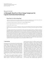
Figure 1: Schematic diagram of an echo canceller.
mitigate this problem, Soo and Pang proposed the multidelay
filtering (MDF) algorithm [15] which uses a block length N
independent of the filter length L. Although it has been well-
known, from the computational complexity point of view,
that N
= L is the optimal choice, the MDF algorithm never-
theless is more efficient than time-domain implementations
even for N<L[16].
In this paper, we propose and evaluate the improved pro-
portionate multidelay filtering (IPMDF) algorithm for sparse
impulse responses.
1
The IPMDF algorithm exploits both the
improvement in convergence brought about by the propor-
tionality control of the IPNLMS algorithm and the efficient
implementation of the MDF structure. As will be explained,
direct extension of the IPNLMS algorithm to the MDF struc-
ture is inappropriate due to the dimension mismatch be-
tween the update vectors. Consequently, in contrast to the
MDF structure, adaptation for the IPMDF algorithm is per-
formed in the time domain. We then evaluate the per for-
mance of IPMDF using impulse responses with various de-

grees of sparseness [18, 19]. This paper is organized as fol-
lows. In Section 2, we review the PNLMS, IPNLMS, and
MDF algorithms. We then derive the proposed IPMDF al-
gorithm in Section 3 while Section 3.2 presents the compu-
tational complexity. Section 4 shows simulation results and
Section 5 concludes our work.
2. ADAPTIVE ALGORITHMS FOR SPARSE
SYSTEM IDENTIFICATION
With reference to Figure 1,wefirstdefinefiltercoefficients
and tap-input vector as

h(n) =


h
0
(n),

h
1
(n), ,

h
L−1
(n)

T
,
x(n)
=


x( n), x(n − 1), , x(n − L +1)

T
,
(1)
where L is the adaptive filter length and the superscript T is
defined as the t ransposition operator. The adaptive filter will
model the unknown impulse response h(n) using the near-
1
An earlier version of this work was presented at the EUSIPCO 2005 special
session on sparse and par tial update adaptive filters [17].
end signal
y(n)
= x
T
(n)h(n)+v(n)+w(n), (2)
where v(n)andw(n) are defined as the near-end speech sig-
nal and ambient noise, respectively. For simplicity, we will
temporarily ignore the effects of double talk and ambient
noise, that is, v(n)
= w(n) = 0, in the description of algo-
rithms.
2.1. The PNLMS and IPNLMS algorithms
The proportionate normalized least mean square (PNLMS)
[5] and improved proportionate normalized least mean
square (IPNLMS) [6] algorithms have been proposed for
network echo cancellation where the impulse response of the
system is sparse. These algorithms can be generalized using
the following set of equations:

e(n)
= y(n) −

h
T
(n − 1)x(n), (3)

h(n) =

h(n − 1) +
μQ(n
− 1)x(n)e(n)
x
T
(n)Q(n − 1)x(n)+δ
,(4)
Q(n
− 1) = diag

q
0
(n − 1), , q
L−1
(n − 1)

,(5)
where μ is the adaptive step-size and δ is the regularization
parameter. The L
× L diagonal control matrix Q(n)deter-
mines the step-size of each filter coefficient and is dependent

on the specific algorithm as described below.
2.1.1. PNLMS
The PNLMS algorithm assigns higher step-sizes for coeffi-
cients with higher magnitude using a control matr ix Q(n).
Elements of the control matrix for PNLMS can be expressed
as [5]
q
l
(n) =
κ
l
(n)

L−1
i
=0
κ
i
(n)
,
κ
l
(n)=max

ρ × max

γ,




h
0
(n)


, ,



h
L−1
(n)



,



h
l
(n)



(6)
with l
= 0, 1, , L − 1 being the tap-indices. The parameter
γ, with a typical value of 0.01, prevents


h
l
(n) from stalling
during initialization stage where

h(0) = 0
L×1
while ρ pre-
vents coefficients from stalling when they are much smaller
than the largest coefficient. The regularization parameter δ
in (4) for PNLMS should be taken as
δ
PNLMS
=
δ
NLMS
L
,(7)
where δ
NLMS
= σ
2
x
is the variance of the input signal [ 6]. It
can be seen that for ρ
≥ 1, PNLMS is equivalent to NLMS.
Andy W. H. Khong et al. 3
2.1.2. IPNLMS
An enhancement of PNLMS is the IPNLMS algorithm [6]
which is a combination of PNLMS and NLMS with the rel-

ative significance of each controlled by a factor α.Theele-
ments of the control matrix Q(n)forIPNLMSaregivenby
q
l
(n) =
1 − α
2L
+(1+α)



h
l
(n)


2

h
1
+ 
,(8)
where
 is a s mall value and ·
1
is the l
1
-norm operator.
It can be seen from the second term of (8) that the magni-
tude of the estimated taps is normalized by the l

1
norm of

h.
This shows that the weighting on the step-size for IPNLMS
is dependent only on the relative scaling of the filter coeffi-
cients as opposed to their absolute values. Results presented
in [6, 17] have shown that good choices of α values are 0,
−0.5, and −0.75. The regularization parameter δ in (4)for
IPNLMS should be taken [6]as
δ
IPNLMS
=
1 − α
2L
δ
NLMS
. (9)
This choice of regularization ensures that the IPNLMS al-
gorithm achieves the same asymptotic steady-state normal-
ized misalignment compared to that of the NLMS algorithm.
It can be seen that IPNLMS is equivalent to NLMS when
α
=−1 while, for α close to 1, IPNLMS behaves like PNLMS.
2.2. The frequency-domain MDF algorithm
Frequency-domain adaptive filtering has been introduced as
aformofimprovingtheefficiency of time-domain algo-
rithms. Although substantial computational savings can be
achieved, one of the main drawbacks of frequency-domain
approaches is the inherent delay introduced [13]. The multi-

delay filtering (MDF) algorithm [15]wasproposedtomiti-
gate the delay problem by partitioning the adaptive filter into
K blocks each having length N such that L
= KN. The MDF
algorithm can be summarized by first letting m be the frame
index and defining the following quantities:
x(mN)
=

x( mN), , x(mN − L +1)

T
, (10)
X(m)
=

x(mN), , x(mN + N − 1)

, (11)
y(m)
=

y(mN), , y(mN + N − 1)

T
, (12)
y(m) =

y(mN), , y(mN + N − 1)


T
= X
T
(m)

h(m),
(13)
e(m)
= y(m) − y(m) =

e(mN), , e(mN + N − 1)

T
.
(14)
We note that X(m) is a Toeplitz matrix of dimension L
× N.
Defining k as the block index and T(m
− k)asanN × N
Toeplitz matrix such that
T(m
− k)
=
⎡
⎢
⎢
⎢
⎢
⎢
⎣

x( mN − kN) ··· x(mN −kN − N +1)
x( mN
− kN +1)
.
.
.
.
.
.
.
.
.
.
.
.
.
.
.
x( mN
− kN + N −1) ··· x(mN −kN)
⎤
⎥
⎥
⎥
⎥
⎥
⎦
,
(15)
it can be shown using (13)and(15) that the adaptive filter

output can be expressed as
y(m) =
K−1

k=0
T(m − k)

h
k
(m), (16)
where

h
k
(m) =


h
kN
(m),

h
kN+1
(m), ,

h
kN+N−1
(m)

T

(17)
is the kth subfilter of

h(m)fork = 0, 1, , K − 1.
It can be shown that the Toeplitz matrix T(m
−k)canbe
transformed, by doubling its size, to a circulant matrix
C(m
− k) =

T

(m − k) T(m − k)
T(m
− k) T

(m − k)

(18)
with
T

(m − k)
=
⎡
⎢
⎢
⎢
⎢
⎢

⎣
x( mN − kN + N) ··· x( mN − kN +1)
x( mN
− kN − N +1)
.
.
.
.
.
.
.
.
.
.
.
.
.
.
.
x( mN
− kN − 1) ··· x(mN −kN + N)
⎤
⎥
⎥
⎥
⎥
⎥
⎦
.
(19)

The resultant circulant matrix C can then be decomposed
[20]as
C
= F
−1
DF, (20)
where F is a 2N
× 2N Fourier matrix and D is a diagonal
matrix whose elements are the discrete Fourier transform of
the first column of C. Note that the diagonal of T

is arbi-
trary, but it is normally equal to the first sample of the previ-
ous block k
− 1[16]. We now define the frequency-domain
quantities:
y
(m) = F

0
N×1
y(m)

,

h
k
(m) = F



h
k
(m)
0
N×1

,
e
(m) = F

0
N×1
e(m)

, G
01
= FW
01
F
−1
,
W
01
=

0
N×N
0
N×N
0

N×N
I
N×N

, G
10
= FW
10
F
−1
,
W
10
=

I
N×N
0
N×N
0
N×N
0
N×N

.
(21)
4 EURASIP Journal on Audio, Speech, and Music Processing
The MDF adaptive algorithm is then given by the following
equations:
e

(m) = y(m) −G
01
×
K−1

k=0
D(m − k)

h
k
(m − 1), (22)
S
MDF
(m) = λS
MDF
(m − 1) + (1 − λ)D
∗
(m)D(m), (23)

h
k
(m) =

h
k
(m − 1) + μG
10
D
∗
(m − k)

×

S
MDF
(m)+δ
MDF

−1
e(m),
(24)
where
∗ denotes complex conjugate, 0  λ<1 is the forget-
ting factor, and μ
= β(1 − λ) is the step-size with 0 <β≤ 1
[16]. It has been found through simulation that this value of
μ exhibits stability in terms of convergence for speech signals.
Letting σ
2
x
be the input signal variance, the initial regular-
ization parameters [16]areS
MDF
(0) = σ
2
x
/100 and δ
MDF
=
20σ
2

x
N/L. For a nonstationary signal, σ
2
x
can be estimated
in a piecewise manner at each iteration by x
T
s
(n)x
s
(n)/(2N)
where x
s
(n) is the first column of the 2N × 2N matrix C.
Convergence analysis for the MDF algorithm is provided in
[21].
3. THE IPMDF ALGORITHM
3.1. Algorithmic formulation
The proposed IPMDF algorithm exploits both the fast con-
vergence of the improved proportionate n ormalized least
mean square (IPNLMS) algorithm and the efficient imple-
mentation of the multidelay adaptive filtering (MDF) algo-
rithm inheriting the beneficial properties of both. We note
that direct use of Q(n), with elements as described by (8),
into the weight update equation in (24) is inappropriate since
the former is in the time domain whereas the latter is in
the frequency domain. Thus our proposed method will be
to update the filter coefficients in the time domain. This is
achieved by first defining the matrices


W
10
=

I
N×N
0
N×N

,

G
10
=

W
10
F
−1
.
(25)
We nex t de fine, for k
= 0, 1, , K −1,
q
k
(m) =

q
kN
(m), q

kN+1
(m), , q
kN+N−1
(m)

(26)
as the partitioned control elements of the kth block such that
each element in this block is now determined by
q
kN+j
(m) =
1 − α
2L
+(1+α)



h
kN+j
(m)


2

h
1
+ 
, (27)
where k
= 0, 1, , K − 1 is the block index while j =

0, 1, , N −1 is the tap-index of each kth block. The IPMDF
algorithm update equation is then given by

h
k
(m) =

h
k
(m − 1) + LμQ
k
(m)

G
10
D
∗
(m − k)
×

S
IPMDF
(m)+δ
IPMDF

−1
e(m),
(28)
δ
IPMDF

=
(1 −α)σ
2
x
20N
2L
λ
=

1 −
1
3L

N
μ = β(1 −λ), 0 <β≤ 1
S
IPMDF
(0) =
(1 −α)σ
2
x
2 ×100

h(0) = 0
L×1

h
k
(m) =



h
kN
(m),

h
kN+1
(m), ,

h
kN+N−1
(m)

T
j = 0, 1, , N − 1
q
kN+j
(m) =
1 −α
2L
+(1+α)



h
kN+j
(m)


2


h
1
+ 
q
k
(m) =

q
kN
(m), q
kN+1
(m), , q
kN+N−1
(m)

Q
k
(m) = diag

q
k
(m)

G
01
= FW
01
F
−1


G
10
=

W
10
F
−1

h
k
(m) = F


h
k
(m)
0
N×1

e(m) = y(m) − G
01
K
−1

k=0
D(m −k)

h

k
(m −1)
S
IPMDF
(m) = λS
IPMDF
(m −1) + (1 −λ)D
∗
(m)D(m)

h
k
(m) =

h
k
(m −1) + LμQ
k
(m)

G
10
D
∗
(m −k)
×

S
IPMDF
(m)+δ

IPMDF

−1
e(m).
Algorithm 1: The IPMDF algorithm.
where the diagonal control matrix Q
k
(m) = diag{q
k
(m)}.
The proposed IPMDF algorithm performs updates in the
time domain by first computing the gradient of the adaptive
algorithm given by D
∗
(m − k)[S
IPMDF
(m)+δ
IPMDF
]
−1
e(m)
in the frequency domain. The matrix

G
10
then converts this
gradient to the time domain so that multiplication with the
(time-domain) control matrix Q
k
(m) is possible. The esti-

mated impulse response

h
k
(m) is then transformed into the
frequency domain for error computation given by
e
(m) = y(m) −G
01
K
−1

k=0
D(m − k)

h
k
(m − 1). (29)
The IPMDF algorithm can be summarized as shown in
Algorithm 1.
3.2. Computational complexity
We consider the computational complexity of the proposed
IPMDF algorithm. We note that although the IPMDF al-
gorithm is updated in the time domain, the er ror e
(m)is
generated using frequency-domain coefficients and hence
five FFT-blocks are required. Since a 2N point FFT re-
quires 2N log
2
N real multiplications, the number of multi-

plications required per output sample for each algorithm is
Andy W. H. Khong et al. 5
described by the following relations:
IPNLMS: 4L,
FLMS: 8 + 10 log
2
L,
MDF: 8K +(4K +6)log
2
N,
IPMDF: 10K +(4K +6)log
2
N.
(30)
It can be seen that the complexity of IPMDF is only mod-
estly higher than MDF. However, as we will see in Section 4,
the performance of IPMDF far exceeds that of MDF for both
speech and white Gaussian noise (WGN) inputs.
4. RESULTS AND DISCUSSIONS
The performance of IPMDF is compared with MDF and
IPNLMS in the context of network echo cancellation. This
performance can be quantified using the normalized mis-
alignment defined by
η(m)
=


h −

h(m)



2
2
h
2
2
, (31)
where
·
2
2
is defined as the squared l
2
-norm operator.
Throughout our simulations, we assume that the length of
the adaptive filter is equivalent to that of the unknown sys-
tem. Results are presented over a single trial and the follow-
ing parameters are chosen for all simulations:
α
=−0.75,
λ
=

1 −
1
(3L)

N
,

β
= 1,
μ
= β × (1 − λ),
S
MDF
(0) =
σ
2
x
100
,
δ
MDF
=
σ
2
x
20N
L
,
S
IPMDF
(0) =
(1 − α)σ
2
x
200
,
δ

IPMDF
=
20(1 − α)σ
2
x
N
(2L)
,
δ
NLMS
= σ
2
x
,
δ
IPNLMS
=
1 − α
2L
δ
NLMS
.
(32)
These choices of parameters allow algorithms to converge to
the same asymptotic value of η(m) for fair comparison.
4.1. Recorded impulse responses
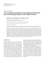
In this first experiment, we investigate the variation of the
rate of convergence with frame size N for IPMDF using
an impulse response of a 64 milliseconds network hybrid
recorded at 8 kHz sampling frequency as shown in Figure 2.

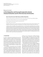
Figure 3 shows the convergence with various frame sizes N
for IPMDF using a white Gaussian noise (WGN) input se-
quence.AnuncorrelatedWGNsequencew(n)isaddedto
0
−0.08
100 200 300 400 500
−0.06
−0.04
−0.02
0.02
0.04
0
Amplitude
Samples
Figure 2: Impulse response of a recorded network hybrid.
0
−40
1234
−30
−20
−10
0
N
= 256
N
= 128
N
= 64
Time (s)
η (dB)

Figure 3: IPMDF convergence for different N with sparse impulse
response. SNR
= 30 dB.
achieve a signal-to-noise ratio (SNR) of 30 dB. It can be seen
that the convergence is faster for smaller N since the adaptive
filter coefficients are being updated more frequently. Addi-
tional simulations for N<64 have indicated that no further
significant improvement in convergence performance is ob-
tained for lower N values.
We compare the relative rate of convergence of the IP-
MDF, MDF, IPNLMS, and NLMS algorithms using the same
impulse response. As before, w(n)isaddedtoachieveanSNR
of 30 dB. The frame size for IPMDF and MDF was chosen to
be N
= 64 while the step-size of IPNLMS and NLMS was
adjusted so that its final misalignment is the same as that for
IPMDF and MDF. This corresponds to μ
IPNLMS
= μ
NLMS
=
0.15. Figure 4 shows the convergence for the respective al-
gorithms using a WGN sequence. It can be seen that there
is a significant improvement in normalized misalignment of
approximately 5 dB during convergence for the IPMDF com-
pared to MDF and IPNLMS.
6 EURASIP Journal on Audio, Speech, and Music Processing
00.511.52 2.53
−40
0

−30
−20
−10
Time (s)
η (dB)
NLMS (μ = 0.15)
MDF
IPNLMS (μ
= 0.15)
IPMDF
Figure 4: Relative convergence of IPMDF, MDF, IPNLMS, and
NLMS using WGN input. SNR
= 30 dB.
0
−45
123456
−40
−30
−25
−20
−15
−10
−5
0
−35
NLMS
IPNLMS
MDF
IPMDF
IPMDF

NLMS
MDF
IPNLMS
Time (s)
η (dB)
Figure 5: Relative convergence of IPMDF, MDF, IPNLMS, and
NLMS using WGN input with echo path change at 3 s. SNR
=30 dB.
We compare the tracking performance of the algorithms
as shown in Figure 5 using a WGN input sequence. In this
simulation, an echo path change, comprising an additional
12-sample delay, was introduced after 3 seconds. As before,
the frame size for the IPMDF and MDF algorithms is N
=
64 while for IPNLMS and NLMS, μ
IPNLMS
= μ
NLMS
=
0.15 is used. We see that IPMDF achieves the highest ini-
tial rate of convergence. When compared with MDF, the
IPMDF algorithm has a higher tracking capability follow-
ing the echo path change at 3 seconds. Compared with the
IPNLMS algorithm, a delay is introduced by block process-
ing the data input for both the MDF and IPMDF algo-
rithms. As a result, IPNLMS achieves a better tracking ca-
pability than the MDF algorithm. The tracking capability
of NLMS is slower compared to IPNLMS and IPMDF due
to its relatively slow convergence rate. Although delay ex-
ists for the IPMDF algorithm, the reduction in delay due

to the multidelay structure allows the IPMDF algorithm to
0
−30
5 1015202530
−25
−20
−15
−10
−5
0
Speech
IPNLMS
MDF
IPMDF
Time (s)
η (dB)
Figure 6: Re lative convergence of IPMDF, MDF, and IPNLMS using
speech input with echo path change at 3 seconds.
achieve an improvement of 2 dB over IPNLMS after echo
path change.
Figure 6 compares the convergence performance of
IPNLMS, IPMDF, and MDF u sing the same experimental
setup as b efore but using a speech input from a male sp eaker.
An echo path change, comprising an additional 12-sample
delay, is introduced at 16 seconds. It can be seen that IP-
MDF achieves approximately 5 dB improvement in normal-
ized misalignment during initial convergence compared to
the MDF algorithm.
4.2. Synthetic impulse responses with various
degrees of sparseness

We illustrate the robustness of IPMDF to impulse response
sparseness. Impulse responses with various degrees of sparse-
ness are generated synthetically using an L
× 1exponentially
decaying window [18]whichisdefinedas
u
=

p 1 e
−1/ψ
, e
−2/ψ
, , e
−(L
u
−1)/ψ

T
, (33)
where the L
p
×1vectorp models the bulk delay a nd is a zero
mean WGN sequence with variance σ
2
p
and L
u
= L − L
p
is

the length of the decaying window while ψ
∈ Z
+
is the decay
constant. Defining an L
u
×1vectorb as a zero mean WGN se-
quence with variance σ
2
b
, the L×1 synthetic impulse response
can then be expressed as
B
= diag{b}, h =

I
L
p
×L
p
0
L
p
×L
u
0
L
u
×L
p

B

u. (34)
The sparseness of an impulse response can be quantified
using the sparseness measure [18, 19]
ξ(h)
=
L
L −
√
L

1 −

h
1
√
Lh
2

. (35)
It has been shown in [18] that ξ(h)reduceswithψ. Figure 7
shows an illustrative example set of impulse responses gen-
erated using (34)withσ
2
p
= 1.055 × 10
−4
, σ
2

b
= 0.9146,
Andy W. H. Khong et al. 7
Amplitude
0 100 200 300 400 512
Samples
−2
−1.5
−0.5
−1
0
0.5
1
1.5
2
(a)
Amplitude
0 100 200 300 400 512
Samples
−2
−1.5
−0.5
−1
0
0.5
1
1.5
2
(b)
Amplitude

0 100 200 300 400 512
Samples
−2
−1.5
−0.5
−1
0
0.5
1
1.5
2
(c)
Amplitude
0 100 200 300 400 512
Samples
−2
−1.5
−0.5
−1
0
0.5
1
1.5
2
(d)
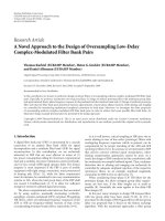
Figure 7: Impulse responses controlled using (a) ψ = 10, (b) ψ = 50, (c) ψ = 150, and (d) ψ = 300 giving sparseness measure (a) ξ = 0.8767,
(b) ξ
= 0.6735, (c) ξ = 0.4216, and (d) ξ = 0.3063.
L = 512, and L
p

= 64. These impulse responses with var ious
degrees of sparseness were generated using decay constants
(a) ψ
= 10, (b) ψ = 50, (c) ψ = 150, and (d) ψ = 300 giv-
ing sparseness measures of (a) ξ
= 0.8767, (b) ξ = 0.6735,
(c) ξ
= 0.4216, and (d) ξ = 0.3063, respectively. We now
investigate the performance of IPNLMS, MDF, and IPMDF
using white Gaussian noise input sequences for impulse re-
sponses generated using 0.3
≤ ξ ≤ 0.9 as controlled by ψ.
As before w(n)isaddedtoachieveanSNRof30dB.Figure 8
shows the variation in time to reach η(m)
=−20 dB nor-
malized misalignment with sparseness measure ξ controlled
using exponential window ψ. Due to the proportional con-
trol of step-sizes, significant increase in the rate of conver-
gence for IPNLMS and IPMDF can be seen as the sparseness
of the impulse responses increases for high ξ. For all cases of
sparseness, the IPMDF algorithm exhibits the highest rate of
convergence compared to IPNLMS and MDF hence demon-
strating the robustness of IPMDF to the sparse nature of the
unknown system.
0
0.40.50.60.70.80.9
0.2
0.4
0.6
0.8

1
(c)
(b)
(a)
Sparseness measure (ξ)
T
20
(s)
Figure 8: Time to reach −20 dB (T
20
) normalized misalignment for
(a) IPNLMS, (b) MDF and (c) IPMDF algorithms with sparseness
measure ξ controlled using exponential decay factor ψ.
8 EURASIP Journal on Audio, Speech, and Music Processing
5. CONCLUSION
We have proposed the IPMDF algorithm for echo cancella-
tion with sparse impulse responses. This algorithm exploits
both the improvement in convergence brought about by the
proportionality control of IPNLMS and the efficient imple-
mentation in the frequency domain of MDF. Simulation re-
sults, using both WGN and speech inputs, have shown that
the improvement in initial convergence and tracking of IP-
MDF over MDF for both sparse and dispersive impulse re-
sponses far outweighs the modest increase in computational
cost.
REFERENCES
[1] J. Radecki, Z. Zilic, and K. Radecka, “Echo cancellation in IP
networks,” in Proceedings of the 45th Midwest Symposium on
Circuits and Systems, vol. 2, pp. 219–222, Tulsa, Okla, USA,
August 2002.

[2] M. Boujida and J M. Boucher, “Higher order statistics applied
to wavelet identification of marine seismic signals,” in Proceed-
ings of European Signal Processing Conference (EUSIPCO ’96),
Trieste, Italy, September 1996.
[3] Y F. Cheng and D. M. Etter, “Analysis of an adaptive technique
for m odeling sparse systems,” IEEE Transactions on Acoustics,
Speech, and Signal Processing, vol. 37, no. 2, pp. 254–264, 1989.
[4] E. A. Robinson and T. S. Durrani, Geophysical Signal Process-
ing, Prentice-Hall, Englewood Cliffs, NJ, USA, 1986.
[5] D. L. Duttweiler, “Proportionate normalized least-mean-
squares adaptation in echo cancelers,” IEEE Transactions on
Speech and Audio Processing, vol. 8, no. 5, pp. 508–518, 2000.
[6] J. Benesty and S. L. Gay, “An improved PNLMS algorithm,”
in Proceedings of IEEE International Conference on Acoustics,
Speech and Signal Processing (ICASSP ’02), vol. 2, pp. 1881–
1884, Orlando, Fla, USA, May 2002.
[7] J. Cui, P. A. Naylor, and D. T. Brown, “An improved I PNLMS
algortihm for echo cancellation in packet-switched networks,”
in Proceedings of IEEE International Conference on Acoustics,
Speech and Signal Processing (ICASSP ’04) , vol. 4, pp. 141–144,
Montreal, Que, Canada, May 2004.
[8] H. Deng and M. Doroslova
ˇ
cki, “New sparse adaptive algo-
rithms using partial update,” in Proceedings of IEEE Interna-
tional Conference on Acoustics, Speech and Signal Processing
(ICASSP ’04), vol. 2, pp. 845–848, Montreal, Que, Canada,
May 2004.
[9] K. Doganc¸ay and O. Tanrikulu, “Adaptive filtering algorithms
with selective partial updates,” IEEE Transactions on Circuits

and Systems II: Analog and Digital Signal Processing, vol. 48,
no. 8, pp. 762–769, 2001.
[10] H. Deng and M. Doroslova
ˇ
cki, “Improving convergence of the
PNLMS algorithm for sparse impulse response identification,”
IEEE Signal Processing Letters, vol. 12, no. 3, pp. 181–184, 2005.
[11] J. W. Cooley and J. W. Tukey, “An a lgorithm for the machine
calculation of complex Fourier series,” Mathematics of Com-
putation, vol. 19, no. 90, pp. 297–301, 1965.
[12] S. Haykin, Adaptive Filter Theory, Information and System Sci-
ence Series, Prentice-Hall, Englewood Cliffs, NJ, USA, 4th edi-
tion, 2002.
[13] J. J. Shynk, “Frequency-domain and multirate adaptive filter-
ing,” IEEE Signal Processing Magazine, vol. 9, no. 1, pp. 14–37,
1992.
[14] E. H
¨
ansler and G. U. Schmidt, “Hands-free telephones - joint
control of echo cancellation and postfiltering,” Signal Process-
ing, vol. 80, no. 11, pp. 2295–2305, 2000.
[15] J S. Soo and K. K. Pang, “Multidelay block frequency domain
adaptive filter,” IEEE Transactions on Acoustics, Speech, and Sig-
nal Processing, vol. 38, no. 2, pp. 373–376, 1990.
[16] J. Benesty, T. G
¨
ansler, D. R. Morgan, M. M. Sondhi, and S.
L. Gay, Advances in Network and Acoustic Echo Cancellation,
Springer, New York, NY, USA, 2001.
[17] A. W. H. Khong, J. Benesty, and P. A. Naylor, “An improved

proportionate multi-delay block adaptive filter for packet-
switched network echo cancellation,” in Proceedings of the 13th
European Signal Processing Conference (EUSIPCO ’05),An-
talya, Turkey, September 2005.
[18] J. Benesty, Y. A. Huang, J. Chen, and P. A. Naylor, “Adap-
tive algorithms for the identification of sparse impulse re-
sponses,” in Selected Methods for Acoustic Echo and Noise Con-
trol,E.H
¨
ansler and G. Schmidt, Eds., chapter 5, pp. 125–153,
Springer, New York, NY, USA, 2006.
[19] P. O. Hoyer, “Non-negative matrix factorization with sparse-
ness constraints,” Journal of Machine Learning Research, vol. 5,
pp. 1457–1469, 2004.
[20] R. Gray, “On the asymptotic eigenvalue distribution of toeplitz
matrices,” IEEE Transactions on Information Theory, vol. 18,
no. 6, pp. 725–730, 1972.
[21] J. Lee and S C. Chong, “On the convergence properties of
multidelay frequency domain adaptive filter,” in Proceedings of
IEEE International Conference on Acoustics, Speech, and Signal
Processing (ICASSP ’99), vol. 4, pp. 1865–1868, Phoenix, Ariz,
USA, March 1999.