Báo cáo hóa học: " Research Article A Hub Matrix Theory and Applications to Wireless Communications" doc

Hindawi Publishing Corporation
EURASIP Journal on Advances in Signal Processing
Volume 2007, Article ID 13659, 8 pages
doi:10.1155/2007/13659
Research Article
A Hub Matrix Theory and Applications to
Wireless Communications
H. T. Kung
1
andB.W.Suter
1, 2
1
Harvard School of Engineering and Applied Scie nces, Harvard University, Cambridge, MA 02138, USA
2
US Air Force Research Laboratory, Rome, NY 13440, USA
Received 24 July 2006; Accepted 22 January 2007
Recommended by Sharon Gannot
This paper considers communications and network systems whose properties are characterized by the gaps of the leading eigen-
values of A
H
A for a matrix A. It is shown that a sufficient and necessary condition for a large eigen-gap is that A is a “hub” matrix
in the sense that it has dominant columns. Some applications of this hub theory in multiple-input and multiple-output (MIMO)
wireless systems are presented.
Copyright © 2007 H. T. Kung and B. W. Suter. This is an open access article distributed under the Creative Commons Attribution
License, which permits unrestricted use, distribution, and reproduction in any medium, provided the original work is properly
cited.
1. INTRODUCTION
There are many communications and network systems whose
properties are characterized by the eigenstructure of a ma-
trix of the form A
H

A, also known as the Gram matrix of A,
where A is a matrix with real or complex entries. For exam-
ple, for a communications system, A couldbeachannelma-
trix, usually denoted H. The capacity of such system is related
to the eigenvalues of H
H
H [1]. In the area of web page rank-
ing, with entries of A representing hyperlinks, Kleinberg [2]
shows that eigenvectors corresponding to the largest eigen-
values of A
T
A give the rankings of the most useful (author-
ity) or popular (hub) web pages. Using a reputation system
that parallels Kleinberg’s work, Kung and Wu [3] developed
an eigenvector-based peer-to-peer (P2P) network user rep-
utation ranking in order to provide services to P2P users
based on past contributions (reputation) to avoid “freeload-
ers.” Furthermore, the rate of convergence in the iterative
computation of reputations is determined by the gap of the
leading two eigenvalues of A
H
A.
The recognition that the eigenstructure of A
H
A deter-
mines the properties of these communications and network
systems motivates the work of this paper. We will develop a
theoretical framework, called a hub matrix theory, which al-
lows us to predict the eigenstructure of A
H

A by examining A
directly. We will prove sufficient and necessary conditions for
the existence of a large gap between the largest and the sec-
ond largest eigenvalues of A
H
A. Finally, we apply the “hub”
theory and our mathematical results to multiple-input and
multiple-output (MIMO) wireless systems.
2. HUB MATRIX THEORY
It is instructive to conduct a thought experiment on a com-
putation process before we introduce our hub matrix the-
ory. The process iteratively computes the values for a set of
variables, which for example could be beamforming weights
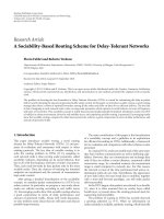
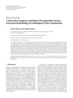
in a beamforming communication system. Figure 1 depicts
an example of this process: variable X uses and contributes
to var iables U
2
and U
4
,variableY uses and contributes to
variables U
3
and U
5
,andvariableZ uses and contributes to
all variables U
1
, , U
6
.WesayvariableZ is a “hub” in the

sense that variables involved in Z’s computation constitute
a superset of those involved in the computation of any other
variable. The dominance is illustrated graphically in Figure 1.
We can describe the computation process in matrix no-
tation. Let
A
=
⎛
⎜
⎜
⎜
⎜
⎜
⎜
⎜
⎜
⎜
⎜
⎝
001
101
011
101
011
001
⎞
⎟
⎟
⎟
⎟

⎟
⎟
⎟
⎟
⎟
⎟
⎠
. (1)
2 EURASIP Journal on Advances in Signal Processing
U
2
U
4
U
3
U
5
X
Y
U
1
U
6
Z
Figure 1: Graphical representation of hub concept.
This process performs two steps alternatively (cf. Figure 1).
(1) X, Y ,andZ contribute to variables in their respective
regions.
(2) X, Y,andZ compute their values using variables in
their respective regions.

The first step (1) is (U
1
, U
2
, , U
6
)
T
← A
∗
(X,Y, Z)
T
and
next step (2) is (X, Y, Z)
T
← A
T∗
(U
1
, U
2
, , U
6
)
T
. Thus, the
computational process performs the iteration (X,Y, Z)
T
←
S

∗
(X,Y, Z)
T
,whereS is defined as follows:
S
= A
T
A =
⎛
⎜
⎝
202
022
226
⎞
⎟
⎠
. (2)
Note that an arrowhead matrix S,asdefinedbelow,has
emerged. Furthermore, note that matrix A exhibits the hub
property of Z in Figure 1 in view of the fact that the last col-
umn of A consists of all 1’s, whereas other columns consist of
only a few 1’s.
Definition 1 (arrowhead matrix). Let S
∈ C
m×m
be a given
Hermitian matrix. S is called an arrowhead matrix if
S
=


Dc
c
H
b

,(3)
where D
= diag(d
(1)
, , d
(m−1)
) ∈ R
(m−1)×(m−1)
is a real di-
agonal matrix, c
= (c
(1)
, , c
(m−1)
) ∈ C
m−1
is a complex
vector , and b
∈ R is a real number.
The eigenvalues of an arbitrary square matrix are invari-
ant under similarity transformations. Therefore, we can with
no loss of generality arrange the diagonal elements of D to be
ordered so that d
(i)

≤ d
(i+1)
for i = 1, , m − 2. For details
concerning arrowhead matrices, see for example [4].
Definition 2 (hub matrix). A matrix A
∈ C
n×m
is called a
candidate-hub matrix,ifm
−1 of its columns are orthogonal
to each other with respect to the Euclidean inner product.
If in addition the remaining column has its Euclidean norm
greater than or equal to that of any other column, then the
matrix A is called a hub matrix and this remaining column
is called the hub column. We are normally interested in hub
matrices where the hub column has much large magnitude
than other columns. (As we show later in Theorems 4 and 10
that in this case the corresponding arrowhead matrices will
have large eigengaps).
In this paper, we study the eigenvalues of S
= A
H
A,where
A is a hub matrix. Since the eigenvalues of S are invariant
under similarity transformations of S, we can permute the
columns of the hub matrix A so that its last column is the hub
column without loss of generality. For the rest of this paper,
we will denote the columns of a hub matrix A by a
1
, , a

m
,
and assume that columns a
1
, , a
m−1
areorthogonaltoeach
other, that is, a
H
i
a
j
= 0fori = j and i, j = 1, , m − 1,
and column a
m
is the hub column. The matrix A introduced
in the context of the graphical model from Figure 1 is such a
hub matrix.
In Section 4, we will relax the orthogonality condition of
a hub matrix, by introducing the notion of hub and arrow-
head dominant matrices.
Theorem 1. Let A
∈ C
n×m
and let S ∈ C
m×m
be the Gram
matrix of A that is, S
= A
H

A. S is an arrowhead matrix if and
only if A is a candidate-hub matrix.
Proof. Suppose A is a candidate-hub matrix. Since S
= A
H
A,
the entries of S are s
(i, j)
= a
H
i
a
j
for i, j = 1, , m.By
Definition 2 of a candidate-hub matrix, the nonhub columns
of A are orthogonal, that is, a
H
i
a
j
= 0fori = j and i, j =
1, , m − 1. Since S is Hermitian, the transpose of the last
column is the complex conjugate of the last row and the di-
agonal elements of S are real numbers. Therefore, S
= A
H
A
is an arrowhead matrix by Definition 1.
Suppose S
= A

H
A is an ar rowhead matrix. Note that the
components of the S matrix of Definition 1 can be repre-
sented in terms of the inner products of columns of A, that
is, b
= a
H
m
a
m
, d
(i)
= a
H
i
a
i
, c
(i)
= a
H
i
a
m
for i = 1, , m − 1.
Since S is an arrowhead matrix, all other off-diagonal entries
of S, s
(i, j)
= a
H

i
a
j
for i = j and i, j = 1, , m − 1, are zero.
Thus, a
H
i
a
j
= 0ifi = j and i, j = 1, , m − 1. So, A is a
candidate-hub mat rix by Definition 2.
Before proving our main result in Theorem 4,wefirstre-
state some well-known results which will be needed for the
proof.
Theorem 2 (interlacing eigenvalues theorem for bordered
matrices). Let U
∈ C
(m−1)×(m−1)
be a given Hermitian ma-
trix, let y
∈ C
(m−1)
be a given vector, and let a ∈ R be a given
real number. Let V
∈ C
m×m
be the Hermitian matrix obtained
by bordering U with y and a as follows:
V
=


Uy
y
H
a

. (4)
Let the eigenvalues of V and U be denoted by
{λ
i
} and {μ
i
},
respectively, and assume that they have been arranged in in-
creasing order, that is, λ
1
≤···≤λ
m
and μ
1
≤···≤μ
m−1
.
Then
λ
1
≤ μ
1
≤ λ
2

≤···≤λ
m−1
≤ μ
m−1
≤ λ
m
. (5)
Proof. See [5, page 189].
Definition 3 (majorizing vectors). Let α ∈ R
m
and β ∈ R
m
begivenvectors.Ifwearrangetheentriesofα and β in
H. T. Kung and B. W. Suter 3
increasing order, that is, α
(1)
≤···≤α
(m)
and β
(1)
≤···≤
β
(m)
, then vector β is said to majorize vector α if
k

i=1
β
(i)
≥

k

i=1
α
(i)
for k = 1, , m (6)
with equality for k
= m.
For details concerning majorizing vectors, see [5,pages
192–198]. The following theorem provides an important
property expressed in terms of vector majorizing.
Theorem 3 (Schur-Horn theorem). Let V
∈ C
m×m
be Her-
mitian. The vector of diagonal entries of V majorizes the vector
of eigenvalues of V.
Proof. See [5, page 193].
Definition 4 (hub-gap). Let A ∈ C
n×m
be a matrix with its
columns denoted by a
1
, , a
m
with 0 < a
1

2
2

≤ ··· ≤

a
m

2
2
.Fori = 1, , m − 1, the ith hub-gap of A is defined
to be
HubGap
i
(A) =


a
m−(i−1)


2
2


a
m−i


2
2
. (7)
Definition 5 (eigengap). Let S

∈ C
m×m
be a Hermitian ma-
trix with its real eigenvalues denoted by λ
1
, , λ
m
with λ
1
≤
···≤
λ
m
.Fori = 1, , m−1, the ith eigengap of S is defined
to be
EigenGap
i
(S) =
λ
m−(i−1)
λ
m−i
. (8)
Theorem 4. Let A
∈ C
n×m
be a hub matrix with its columns
denoted by a
1
, , a

m
and 0 < a
1

2
2
≤···≤a
m

2
2
.LetS =
A
H
A ∈ C
m×m
be the corresponding arrowhead matrix with its
eigenvalues denoted by λ
1
, , λ
m
w ith 0 ≤ λ
1
≤ ··· ≤ λ
m
.
Then
HubGap
1
(A) ≤ EigenGap

1
(S)
≤

HubGap
1
(A)+1

HubGap
2
(A).
(9)
Proof. Let T be the mat rix formed from S by deleting its
last row and column. This means that T is a diagonal ma-
trix with diagonal elements
a
i

2
2
for i = 1, , m − 1. By
Theorem 2, the eigenvalues of S interlace those of T, that
is, λ
1
≤a
1

2
2
≤ ··· ≤ λ

m−1
≤a
m−1

2
2
≤ λ
m
.Thus,
λ
m−1
is a lower bound for a
m−1

2
2
.ByTheorem 3, the vec-
tor of diagonal values of S majorizes the vector of eigenval-
ues of S, that is,

k
i=1
d
(i)
≥

k
i=1
λ
i

for k = 1, , m − 1and

m−1
i
=1
d
(i)
+ b =

m
i
=1
λ
m
.So,b ≤ λ
m
. Since b =a
m

2
2
,
λ
m
is an upper bound for a
m

2
2
.Hence,a

m

2
2
/a
m−1

2
2
≤
λ
m
/λ
m−1
or HubGap
1
(A) ≤ EigenGap
1
(S).
Again, by using Theorems 2 and 3,wehave

m−1
i
=1
d
(i)
+
b
=


m
i=1
λ
m
and λ
1
≤ d
(1)
≤ λ
2
≤ d
(2)
≤ λ
3
≤ ··· ≤
d
(m−2)
≤ λ
m−1
≤ d
(m−1)
≤ λ
m
, and, as such,

d
(1)
+ ···+ d
(m−2)


+ d
(m−1)
+ b
= λ
1
+

λ
2
+ ···+ λ
m−1

+ λ
m
≥ λ
1
+

d
(1)
+ ···+ d
(m−2)

+ λ
m
.
(10)
This result implies that d
(m−1)
+ b ≥ λ

1
+ λ
m
≥ λ
m
. By noting
that d
(m−2)
≤ λ
m−1
,wehave
EigenGap
1
(S) =
λ
m
λ
m−1
≤
d
(m−1)
+ b
d
(m−2)
=


a
m−1



2
2
+


a
m


2
2


a
m−2


2
2
=


a
m−1


2
2



a
m−2


2
2
+


a
m


2
2


a
m−1


2
2
·


a
m−1



2
2


a
m−2


2
2
=

HubGap
1
(A)+1

·
HubGap
2
(A).
(11)
By Theorem 4, we have the following result, where nota-
tion “
” means “much larger than.”
Corollary 1. Let A
∈ C
n×m
be a matrix with its columns
a

1
, , a
m
satisfying 0 < a
1

2
2
≤ ··· ≤ a
m−1

2
2
≤a
m

2
2
.
Let S
= A
H
A ∈ C
m×m
with its eigenvalues λ
1
, ···, λ
m
satisfy-
ing 0

≤ λ
1
≤···≤λ
m
.Thefollowingholds
(1) if A is a hub matrix with
a
m

2
a
m−1

2
, then S
is an arrowhead matrix with λ
m
 λ
m−1
;and
(2) if S is an arrowhead matrix with λ
m
 λ
m−1
, then A
is a hub matrix with
a
m

2

a
m−1

2
or a
m−1

2


a
m−2

2
or both.
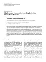
3. MIMO COMMUNICATIONS APPLICATION
A multiple-input multiple-output (MIMO) system with M
t
transmit antennas and M
r
receive antennas is depicted in
Figure 2 [6, 7]. Assume the MIMO channel is modeled by
the M
r
× M
t
channel propagation matrix H = (h
ij
). The
input-output relationship, given a transmitted symbol s,for

thissystemisgivenby
x
= sz
H
Hw + z
H
n. (12)
The vectors w and z in the equation are called the beamform-
ing and combining vectors, respectively, which will be chosen
to maximize the signal-to-noise ratio (SNR). We will model
the noise vector n as having entries, which are independent
and identically distributed (i.i.d.) random variables of com-
plex Gaussian distribution CN(0, 1). Without loss of gener-
ality, assume the average power of transmit signal equals one,
that is, E
|s|
2
= 1. For the beamforming system described
here, the signal to noise ratio, γ, after combining at the re-
ceiver is given by
γ
=


z
H
Hw


2

z
2
2
. (13)
Without loss of generality, assume
z
2
= 1. With this as-
sumption, the SNR becomes
γ
=


z
H
Hw


2
. (14)
4 EURASIP Journal on Advances in Signal Processing
Coding
and
modulation
n
M
r
−1
z
∗

M
r
−1
n
M
r
z
∗
M
r
Bit
stream
w
1
w
2
w
M
t
−1
w
M
t
h
1,M
t
h
M
r
−1,2

s
n
2
z
∗
2
n
1
z
∗
1
x
.
.
.
.
.
.
Figure 2: MIMO block diagram (see [6, datapath portion of Figure 1]).
3.1. Maximum ratio combining
Areceiverwherez maximizes γ for a given w is known as a
maximum ratio combining (MRC) receiver in the literature.
By the Cauchy-Bunyakovskii-Schwartz inequality (see, e.g.,
[8, page 272]), we have


z
H
Hw



2
≤z
2
2
Hw
2
2
. (15)
Since we already assume
z
2
= 1,


z
H
Hw


2
≤Hw
2
2
. (16)
Moreover, since in MRC we desire to maximize the SNR, we
must choose z to be
z
MRC
=

Hw
Hw
2
, (17)
which implies that the SNR for MRC is
γ
MRC
=Hw
2
2
. (18)
3.2. Selection diversity transmission,
generalized subset selection, and
combined SDT/MRC and GSS/MRC
For a selection diversity transmission (SDT) [9]system,only
the antenna that yields the largest SNR is selected for trans-
mission at any instant of time. This means
w
=

δ
1, f (1)
, , δ
M
t
, f (1)

T
, (19)
where the Kronecker impulse δ

i, j
is defined as δ
i, j
= 1ifi = j,
and δ
i, j
= 0ifi = j,and f (1) represents the value of the in-
dex x that maximizes

i
|h
i,x
|
2
. Thus, the SNR for the com-
bined SDT/MRC communications system is
γ
SDT/MRC
=


h
f (1)


2
2
. (20)
By definition, a generalized subset selection (GSS) [10]sys-
tem powers those k transmitters which yield the top k

SNR values at the receiver for some k>1. That is, if
f (1), f (2), , f (k) stand for the indices of these transmit-
ters, then w
f (i)
= 1/
√
k for i = 1, , k, and all other entries
of w are zero. It follows that, for the combined GSS/MRC
communications system, the SNR gain is given by
γ
GSS/MRC
=
1
k





k

i=1
h
f (i)





2

2
. (21)
In the limiting case when k
= M
t
,GSSbecomesequalgain
transmission (EGT) [6, 7], which requires all M
t
transmit-
ters to be equally powered, that is, w
f (i)
= 1/

M
t
for i =
1, , M
t
. Then, for the combined EGT/MRC communica-
tions system, the SNR gain takes the expression
γ
EGT/MRC
=
1
M
t






M
t

i=1
h
f (i)





2
2
. (22)
3.3. Maximum ratio transmission and
combined MRT/MRC
Suppose there are no constraints placed on the form of the
vector w. Let us reexamine the expression of SNR gain γ
MRC
.
Note
γ
MRC
=Hw
2
2
= (Hw)
H
(Hw) = w

H

H
H
Hw

. (23)
With the assumption that
w
2
= 1, the above equation is
maximized under maximum ratio transmission (MRT) [9]
(see, e.g., [5, page 295]), that is, when
w
= w
m
, (24)
where w
m
is the normalized eigenvector corresponding to the
largest eigenvalues λ
m
of H
H
H. Thus, for an MRT/MRC sys-
tem, we have
γ
MRT/MRC
= λ
m

. (25)
H. T. Kung and B. W. Suter 5
3.4. Performance comparison between
SDT/MRC and MRT/MRC
Theorem 5. Let H
∈ C
n×m
be a hub matrix with its columns
denoted by h
1
, , h
m
and 0 < h
1

2
2
≤···≤h
m−1

2
2
≤

h
m

2
2
.Letγ

SDT/MRC
and γ
MRT/MRC
be the SNR gains for
SDT/MRC and MRT/MRC, respectively. Then
HubGap
1
(H)
HubGap
1
(H)+1
≤
γ
SDT/MRC
γ
MRT/MRC
≤ 1. (26)
Proof. We note that the A matrix in hub matrix theory of
Section 2 corresponds to the H matrix here, and the a
i
col-
umn of A corresponds to the h
i
column of H for i = 1, , m.
From the proof of Theorem 4,wenoteb
=a
m

2
2

≤ λ
m
or
h
m

2
2
≤ λ
m
. It follows that
γ
SDT/MRC
γ
MRT/MRC
≤ 1. (27)
To derive a l ower b o u n d for γ
SDT/MRC
/γ
MRT/MRC
,wenote
from the proof of Theorem 4 that λ
m
≤ d
(m−1)
+ b. This
means that
γ
MRT/MRC
≤



a
m−1


2
2
+


a
m


2
2
=


h
m−1


2
2
+


h

m


2
2
. (28)
Thus
γ
SDT/MRC
γ
MRT/MRC
≥


h
m


2
2


h
m−1


2
2
+



h
m


2
2
=
HubGap
1
(H)
HubGap
1
(H)+1
.
(29)
The inequality γ
SDT/MRC
/γ
MRT/MRC
≤ 1inTheorem 5 ref-
lects the fact that in the SDT/MRC system, w is cho-
sen to be a particular unit vector rather than an optimal
choice. The other inequality of Theorem 5, HubGap
1
(H)/
(HubGap
1
(H)+1) ≤ γ
SDT/MRC

/γ
MRT/MRC
, implies that the
SNR for SDT/MRC approaches that for MRT/MRC when H
is a hub matrix with a dominant hub column. More precisely,
we have the following result.
Corollary 2. Let H
∈ C
n×m
be a hub matrix with its
columns denoted by h
1
, , h
m
and 0 < h
1

2
2
≤ ··· ≤

h
m

2
2
.Letγ
SDT/MRC
and γ
MRT/MRC

be the SNR for SDT/MRC
and MRT/MRC, respectively. Then, as HubGap
1
(H) increases,
γ
MRT/MRC
/γ
SDT/MRC
approaches one at a rate of at least
HubGap
1
(H)/(HubGap
1
(H)+1).
3.5. GSS-MRT/MRC and performance comparison
with MRT/MRC
Using an analysis similar to the one above, we can derive per-
formance bounds for a recently discovered communication
system that incorporates antenna selection with MRT on the
transmission side while applying MRC on the receiver side
[11, 12]. This approach will be called GSS-MRT/MRC here.
Given a GSS scheme that powers those k transmitters which
yield the top k highest SNR values, a GSS-MRT/MRC sys-
tem is defined to be an MRT/MRC system applied to these k
transmitters. Let f (1), f (2), , f (k) be the indices of these
k transmitters, and

H the matrix formed by columns h
f (i)
of

H for i
= 1, , k. It is easy to see that the SNR for GSS-
MRT/MRC is
γ
GSS-MRT/MRC
=

λ
m
, (30)
where

λ
m
is the largest eigenvalue of

H
H

H.
Theorem 6. Let H
∈ C
n×m
be a hub matrix with its columns
denoted by h
1
, , h
m
and 0 < h
1


2
2
≤ ··· ≤ h
m−1

2
2
≤

h
m

2
2
.Letγ
GSS−MRT/MRC
and γ
MRT/MRC
be the SNR values for
GSS-MRT/MRC and MRT/MRC, respectively. Then
HubGap
1
(H)
HubGap
1
(H)+1
≤
γ
GSS−MRT/MRC

γ
MRT/MRC
≤
HubGap
1
(H)+1
HubGap
1
(H)
.
(31)
Proof. Since 0 <
h
1

2
2
≤···≤h
m−1

2
2
≤h
m

2
2
,

H con-

sists of the last k columns of H. Moreover, since H is a hub
matrix, so is

H. From the proof of Theorem 4, we note both
λ
m
and

λ
m
are bounded above by h
m−1

2
2
+h
m

2
2
and below
by
h
m

2
2
. It follows that
HubGap
1

(H)
HubGap
1
(H)+1
=


h
m


2
2


h
m−1


2
2
+


h
m


2
2

≤
γ
GSS−MRT/MRC
γ
MRT/MRC
=

λ
m
λ
m
≤


h
m−1


2
2
+


h
m


2
2



h
m


2
2
=
HubGap
1
(H)+1
HubGap
1
(H)
.
(32)
3.6. Diversity selection with partitions,
DSP-MRT/MRC, and performance b ounds
Suppose that transmitters are partitioned into multiple
transmission partitions. We define the diversity selection
with partitions (DSP) to be the transmission scheme where
in each transmission partition only the transmitter with the
largest SNR will be powered. Note that SDT discussed above
is a special case of DSP when there is only one partition con-
sisting of all transmitters.
Let k be the number of partitions, and f (1), f (2),
, f (k) the indices of the powered transmitters. A DSP-
MRT/MRCsystemisdefinedtobeanMRT/MRCsystem
applied to these k transmitters. Define


H to be the matrix
formed by columns h
f (i)
of H for i = 1, , k. Then the SNR
for DSP-MRT/MRC is
γ
DSPS-MRT/MRC
=

λ
m
, (33)
where

λ
m
is the largest eigenvalue of

H
H

H.
Note that in general the powered transmitters for DSP
are not the same as those for GSS. This is because a trans-
mitter that yields the highest SNR among transmitters in
one of the k partitions may not be among the transmit-
ters that yield the top k highest SNR values among all
transmitters. Nevertheless, when H is a hub matrix with
6 EURASIP Journal on Advances in Signal Processing
0 < h

1

2
2
≤ ··· ≤ h
m−1

2
2
≤h
m

2
2
,wecanbound

λ
m
for DSP-MRT/MRC in a manner similar to how we bound

λ
m
for GSS-MRT/MRC. That is, for DSP-MRT/MRC,

λ
m
is
bounded above by
h
k


2
2
+h
m

2
2
and below by h
m

2
2
,where
h
k
is the second largest column of

H in magnitude. Note that
h
k

2
2
≤h
m−1

2
2
, since the second largest column of


H in
magnitude cannot be larger that than of H. We have the fol-
lowing result similar to that of Theorem 6.
Theorem 7. Let H
∈ C
n×m
be a hub matrix with its columns
denoted by h
1
, , h
m
and 0 < h
1

2
2
≤···≤h
m−1

2
2
≤

h
m

2
2
.Letγ

DSP−MRT/MRC
and γ
MRT/MRC
be the SNR for DSP-
MRT/MRC and MRT/MRC, respectively. Then
HubGap
1
(H)
HubGap
1
(H)+1
≤
γ
DSP−MRT/MRC
γ
MRT/MRC
≤
HubGap
1
(H)+1
HubGap
1
(H)
.
(34)
Theorems 6 and 7 imply that when HubGap
1
(H) becomes
large, the SNR values of both GSS-MRT/MRC and DSP-
MRT/MRC approach that of MRT/MRC.

4. HUB DOMINANT MATRIX THEORY
We generalize the hub matrix theory presented above to situ-
ations when matrix A (or H) exhibits a “near” hub property.
In order to relax the definition of orthogonality of a set of
vectors, we use the notion of frame.
Definition 6 (frame). A set of distinct vectors
{f
1
, , f
n
} is
said to be a frame if there exist positive constants ξ and ϑ
called frame bounds such that
ξ


f
j


2
≤
n

i=1


f
H
i

f
j


≤
ϑ


f
j


2
for j = 1, , n. (35)
Note that if ξ
= ϑ = 1, then the set of vectors {f
1
, , f
n
}
is orthogonal. Here we use frames to bound the non-
orthogonality of a collection of vectors, while the usual use
for frames is to quantify the redundancy in a representation
(see, e.g., [13]).
Definition 7 (hub dominant matr ix). A matrix A
∈ C
n×m
is called a candidate-hub-dominant mat rix if m − 1ofits
columns form a frame with frame bounds ξ
= 1andϑ = 2,

that is,
a
j

2
≤

m−1
i
=1
|a
H
i
a
j
|≤2a
j

2
for j = 1, , m − 1.
If in addition the remaining column has its Euclidean norm
greater than or equal to that of any other column, then the
matrix A is called a hub-dominant matrix and the remaining
column is called the hub column.
We next generalize the definition of arrowhead matrix
to arrowhead dominant matrix, where the matrix D in
Definition 1 goes from being a diagonal matrix to a diago-
nally dominant matrix.
Definition 8 (diagonally dominant mat rix). Let E
∈ C

m×m
be a given Hermitian matrix. E is said to be diagonally dom-
inant if for each row the magnitude of the diagonal entry is
greater than or equal to the row sum of magnitudes of all
off-diagonal entries, that is,


e
(i,i)


≥
m−1

j=1
j
=i


e
(i, j)


for i = 1, , m. (36)
For more information on diagonally dominant matrices, see
for example [5, page 349].
Definition 9 (arrowhead dominant matrix). Let S
∈ C
m×m
be

a given Hermitian matrix. S is called an arrowhead dominant
matrix if
S
=

Dc
c
H
b

, (37)
where D
∈ C
(m−1)×(m−1)
is a diagonally dominant matrix,
c
= (c
(1)
, , c
(m−1)
) ∈ C
m−1
is a complex vector, and b ∈ R
is a real number.
Similar to Theorem 1, we have the following theorem.
Theorem 8. Let A
∈ C
n×m
and let S ∈ C
m×m

be the Gram
matrix of A,thatis,S
= A
H
A. S is an arrowhead dominant
matrix if and only if A is a candidate-hub-dominant matrix.
Proof. Suppose A is a candidate-hub-dominant matrix. Since
S
= A
H
A, the entries of S can be expressed as s
(i, j)
= a
H
i
a
j
for
i, j
= 1, , m.ByDefinition 7 of a hub-dominant matrix,
the nonhub columns of A form a frame with frame bounds
ξ
= 1andϑ = 2, that is a
j

2
≤

m−1
i=1

|a
H
i
a
j
|≤2a
j

2
for j = 1, , m − 1. Since a
j

2
=|a
H
j
a
j
|, it follows that
|a
H
i
a
i
|≥

m−1
j=1, j=i
|a
H

i
a
j
|, i = 1, , m − 1, which is the diag-
onal dominance condition on the sub-matr ix D of S. Since S
is Hermitian, the transpose of the last column is the complex
conjugate of the last row and the diagonal elements of S are
real numbers. Therefore, S
= A
H
A is an arrowhead domi-
nant matrix in accordance with Definition 9.
Suppose S
= A
H
A is an arrowhead dominant matrix.
Note that the components of the S matrix of Definition 9 can
be represented in terms of the columns of A.Thusb
= a
H
m
a
m
and c
(i)
= a
H
i
a
m

for i = 1, , m − 1. Since |a
H
j
a
j
|=a
j

2
,
the diagonal dominance condition,
|a
H
i
a
i
|≥

m−1
j
=1, j=i
|a
H
i
a
j
|,
i
= 1, , m −1, implies that a
j


2
≤

m−1
i
=1
|a
H
i
a
j
|≤2a
j

2
for j = 1, , m −1. So, A is a candidate-hub-dominant ma-
trix by Definition 7.
Before proceeding to our results in Theorem 10,wewill
first restate a well-known result which will be needed for the
proof.
Theorem 9 (monotonicity theorem). Let G, H
∈ C
m×m
be
Hermitian. Assume H is positive semidefinite and that the
eigenvalues of G and G + H are arranged in increasing order,
that is, λ
1
(G) ≤ ··· ≤ λ

m
(G) and λ
1
(G + H) ≤···≤
λ
m
(G + H). Then λ
κ
(G) ≤ λ
k
(G + H) for k = 1, , m.
Proof. See [5, page 182].
H. T. Kung and B. W. Suter 7
Theorem 10. Let A ∈ C
n×m
be a hub-dominant matrix with
its columns denoted by a
1
, , a
m
w ith 0 < a
1

2
≤ ··· ≤

a
m−1

2

≤a
m

2
.LetS = A
H
A ∈ C
m×m
be the correspond-
ing arrowhead dominant mat rix with its eigenvalues denoted
by λ
1
, , λ
m
w ith λ
1
≤ ··· ≤ λ
m
.Letd
(i)
and σ
(i)
denote
the diagonal entry and the sum of magnitudes of off-diagonal
entries, respectively, in row i of S for i
= 1, , m. Then
(a) HubGap
1
(A)/2 ≤ EigenGap
1

(S),and
(b) EigenGap
1
(S) = λ
m
/λ
m−1
≤ (d
(m−1)
+ b +

m−2
i=1
σ
(i)
)/(d
(m−2)
− σ
(m−2)
).
Proof. Let T be the matrix formed from S by deleting its last
row and column. This means that T is a diagonally dominant
matrix. Let the eigenvalues of T be
{μ
i
} with μ
1
≤ ··· ≤
μ
m−1

. Then by Theorem 9,wehaveλ
1
≤ μ
1
≤ λ
2
≤ ··· ≤
λ
m−1
≤ μ
m−1
≤ λ
m
. Applying Gershgorin’s theorem to T and
noting that T is a diagonally dominant with d
(m−1)
being its
largest diagonal entry, we have μ
m−1
≤ 2d
(m−1)
.Thusλ
m−1
≤
2d
(m−1)
= 2a
m−1

2

2
. As observed in the proof of Theorem 4,
λ
m
≥ b =a
m

2
2
. Therefore, a
m

2
2
/(2a
m−1

2
2
) ≤ λ
m
/λ
m−1
or HubGap
1
(A)/2 ≤ EigenGap
1
(S).
Let E be the matrix formed from T with its diagonal en-
tries replaced by the corresponding off-diagonal row sums,

and let
T = T −E. Since T is a diagonally dominant matrix,
T is a diagonal mat rix with nonnegative diagonal entries. Let
the diagonal entries of
T be {d
(i)
}. Then d
(i)
= d
(i)
− σ
(i)
.
Assume that
d
(1)
≤···≤d
(m−1)
. Since E is a sy mmetric di-
agonally dominant matrix with positive diagonal entries, it is
a positive semidefinite matrix. Since T
= T+E,byTheorem 9
we have μ
i
≥ d
(i)
for i = 1, , m − 1. Let
S
=


Dc
c
H
b

(38)
in accordance w ith Definition 9.ByTheorem 3,wehave

m−1
i
=1
d
(i)
+ b =

m
i
=1
λ
m
. Thus, by noting λ
1
≤ μ
1
≤ λ
2
≤
···≤
λ
m−1

≤ μ
m−1
≤ λ
m
,wehave
d
(1)
+ d
(2)
+ ···+ d
(m−1)
+ b
= λ
1
+ λ
2
+ ···+ λ
m
≥ λ
1
+ μ
1
+ ···+ μ
m−2
+ λ
m
≥ λ
1
+ d
(1)

+ ···+ d
(m−2)
+ λ
m
.
(39)
This implies that d
(m−1)
+b+

m−2
i
=1
σ
(i)
≥ λ
1
+λ
m
≥ λ
m
. Since
d
(m−2)
− σ
(m−2)
= d
(m−2)
≤ μ
m−2

≤ λ
m−1
,wehave
EigenGap
1
(S) =
λ
m
λ
m−1
≤
d
(m−1)
+ b +

m−2
i
=1
σ
(i)
d
(m−2)
− σ
(m−2)
. (40)
Note that if there exist positive numbers p and q,with
q<1, such that (1
− q)d
(m−2)
≥ σ

(m−2)
and
p

d
(m−1)
+ b

≥
m−2

i=1
σ
(i)
, (41)
then the inequality (b) in Theorem 10 implies
λ
m
λ
m−1
≤ r ·
d
(m−1)
+ b
d
(m−2)
, (42)
where r
= (1 + p)/q. As in the end of the proof of Theorem 4,
it follows that

EigenGap
1
(S) ≤ r ·

HubGap
1
(A)+1

· HubGap
2
(A).
(43)
This together with (a) in Theorem 10 gives the following re-
sult.
Corollary 3. Let A
∈ C
n×m
be a matrix with its columns
a
1
, , a
m
satisfying 0 < a
1

2
2
≤ ··· ≤ a
m−1


2
2
≤a
m

2
2
.
Let S
= A
H
A ∈ C
m×m
be a Hermitian matrix with its eigen-
values λ
1
, , λ
m
satisfying 0 ≤ λ
1
≤···≤λ
m
. The following
holds
(1) if A is a hub-dominant matrix with
a
m

2



a
m−1

2
, then S is an arrowhead dominant matrix with
λ
m
 λ
m−1
;and
(2) if S is an arrowhead dominant matrix with λ
m

λ
m−1
,andifp(d
(m−1)
+ b) ≥

m−2
i
=1
σ
(i)
and (1 −
q)d
(m−2)
≥ σ
(m−2)

for some positive numbers p and
q with q<1, then A is a hub-dominant matr ix with
a
m

2
a
m−1

2
or a
m−1

2
a
m−2

2
or both.
Sometimes, especially for large-dimensional matrices, it
is desirable to relax the notion of diagonal dominance. This
can be done using arguments analogous to those given above
(see, e.g., [14]), and extensions represent an open research
problem for the future.
5. CONCLUDING REMARKS
This pap er has presented a hub matrix theory and applied it
to beamforming MIMO communications systems. The fact
that the performance of the MIMO beamforming scheme is
critically related to the gap between the two largest eigenval-
ues of the channel propagation matrix is well known, but this

paper reported for the first time how to obtain this insight di-
rectly from the structure of the matrix, that is, its hub prop-
erties. We believe that numerous communications systems
might be well descr ibed within the formalism of hub matri-
ces. As an example, one can consider the problem of nonco-
operative beamforming in a wireless sensor network, where
several source (transmitting) nodes communicate with a des-
tination node, but only one source node is located in the
vicinity of the destination node and presents a direct line-of-
sight to the destination node. Extending the hub matrix for-
malism to other types of matrices (e.g., matrices with a clus-
ter of dominant columns) represents an interesting open re-
search problem. The contributions reported in this paper can
be extended further to treat the more general class of block
arrowhead and hub dominant matrices that enable the anal-
ysis and design of a lgorithms and protocols in areas such as
distributed beamforming and power control in wireless ad-
hoc networks. By relaxing the diagonal-matrix condition, in
8 EURASIP Journal on Advances in Signal Processing
the definition of an arrowhead matrix, with a block diagonal
condition, and enabling groups of columns to be correlated
or uncorrelated (orthogonal/nonorthogonal) in the defini-
tion of block dominant hub matrices, a much larger spec-
trum of applications could be treated within the proposed
framework.
ACKNOWLEDGMENTS
The authors wish to acknowledge discussions that occurred
between the authors and Dr. Michael Gans. These discus-
sions significantly improved the quality of the paper. In ad-
dition, the authors wish to thank the reviewers for their

thoughtful comments and insightful observations. This re-
search was supported in part by the Air Force Office of Sci-
entific Research under Contract FA8750-05-1-0035 and by
the Information Directorate of the Air Force Research Labo-
ratory and in part by NSF Grant no.ACI-0330244.
REFERENCES
[1] D.TseandP.Viswanath,Fundamentals of Wireless Communi-
cation, Cambridge University Press, Cambridge, UK, 2005.
[2] J. M. Kleinberg, “Authoritative sources in a hyperlinked envi-
ronment,” in Proceedings of the 9th Annual ACM-SIAM Sym-
posium on Discrete Algorithms, pp. 668–677, San Francisco,
Calif, USA, January 1998.
[3] H.T.KungandC H.Wu,“Differentiated admission for peer-
to-peer systems: incentivizing peers to contribute their re-
sources,” in Workshop on Economics of Peer-to-Peer Systems,
Berkeley, Calif, USA, June 2003.
[4] D. P. O’Leary and G. W. Stewart, “Computing the eigenvalues
and eigenvectors of symmetric arrowhead matrices,” Journal of
Computational Physics, vol. 90, no. 2, pp. 497–505, 1990.
[5] R. A. Horn and C. R. Johnson, Matrix Analysis, Cambridge
University Press, Cambridge, UK, 1985.
[6] D. J. Love and R. W. Heath Jr., “Equal gain transmission in
multiple-input multiple-output wireless systems,” IEEE Trans-
actions on Communications, vol. 51, no. 7, pp. 1102–1110,
2003.
[7]D.J.LoveandR.W.HeathJr.,“Correctionsto“Equalgain
transmission in multiple-input multiple-output wireless sys-
tems”,” IEEE Transactions on Communications,vol.51,no.9,
p. 1613, 2003.
[8] C. D. Meyer, Matrix Analysis and Applied Linear Algebra,

SIAM, Philadelphia, Pa, USA, 2000.
[9] C H. Tse, K W. Yip, and T S. Ng, “Performance tradeoffs
between maximum ratio transmission and switched-transmit
diversity,” in Proceedings of the 11th IEEE International Sym-
posium on Personal, Indoor and Mobile Radio Communications
(PIMRC ’00), vol. 2, pp. 1485–1489, London, UK, September
2000.
[10]D.J.Love,R.W.HeathJr.,andT.Strohmer,“Grassman-
nian beamforming for multiple-input multiple-output wire-
less systems,” IEEE Transactions on Information Theory, vol. 49,
no. 10, pp. 2735–2747, 2003.
[11] C. Murthy and B. D. Rao, “On antenna selection with max-
imum ratio transmission,” in Conference Record of the 37th
Asilomar Conference on Signals, Systems and Computers, vol. 1,
pp. 228–232, Pacific Grove, Calif, USA, November 2003.
[12] A. F. Molisch, M. Z. Win, and J. H. Winter, “Reduced-
complexity transmit/receive-diversity systems,” IEEE Transac-
tions on Signal Processing, vol. 51, no. 11, pp. 2729–2738, 2003.
[13] R. M. Young, An Introduction to Nonharmonic Fourier Series,
Academic Press, New York, NY, USA, 1980.
[14] N. Sebe, “Diagonal dominance and integrity,” in Proceedings
of the 35th IEEE Conference on Decision and Control, vol. 2, pp.
1904–1909, Kobe, Japan, December 1996.
H. T. Kung received his B.S. degree from
National Tsing Hua University (Taiwan),
and Ph.D. degree from Carnegie Mellon
University. He is currently William H. Gates
Professor of computer science and electrical
engineering at Harvard University. In 1999
he started a joint Ph.D. program with col-

leagues at the Harvard Business School on
information, technology, and management,
and cochaired this Harvard program from
1999 to 2006. Prior to joining Harvard in 1992, Dr. Kung taught at
Carnegie Mellon, pioneered the concept of systolic array process-
ing, and led large research teams on the design and development
of novel computers and networks. Dr. Kung has pursued a variety
of research interests over his career, including complexity theory,
database systems, VLSI design, parallel computing, computer net-
works, network security, wireless communications, and networking
of unmanned aerial systems. He maintains a strong linkage with
industry and has served as a Consultant and Board Member to nu-
merous companies. Dr. Kung’s professional honors include Mem-
ber of the National Academy of Engineering in USA and Member
of the Academia Sinica in Taiwan.
B. W. Suter received the B.S. and M.S.
degrees in electrical engineering in 1972
andthePh.D.degreeincomputerscience
in 1988, all from the University of South
Florida, Tampa, FLa. Since 1998, he has
been with the Information Directorate of
the Air Force Research Laboratory, Rome,
NY, where he is the Founding Director of
the Center for Integrated Transmission and
Exploitation. Dr. Suter has authored over a
hundred publications and the author of the book Multirate and
Wavelet Signal Processing (Academic Press, 1998). His research in-
terests include multiscale signal and image processing, cross layer
optimization, networking of unmanned aerial systems, and wireless
communications. His professional background includes industrial

experience with Honeywell Inc., St. Petersburg, FLa, and with Lit-
ton Industries, Woodland Hills, Calif, and academic experience at
the University of Alabama, Birmingham, Aa and at the Air Force In-
stitute of Technology, Wright-Patterson AFB, Oio. Dr. Suter’s hon-
ors include Air Force Research Laboratory Fellow, the Arthur S.
Flemming Award: Science Category, and the General Ronald W.
Yates Award for Excellence in Technology Transfer. He served as an
Associate Editor of the IEEE Transactions on Signal Processing. Dr.
Suter is a Member of Tau Beta P i and Eta Kappa Nu.