Báo cáo hóa học: " Research Article Construction of Orthonormal Piecewise Polynomial Scaling and Wavelet Bases on Non-Equally Spaced Knots" docx

Hindawi Publishing Corporation
EURASIP Journal on Advances in Signal Processing
Volume 2007, Article ID 27427, 13 pages
doi:10.1155/2007/27427
Research Article
Construction of Orthonormal Piecewise Polynomial Scaling
and Wavelet Bases on Non-Equally Spaced Knots
Anissa Zerga
¨
ınoh,
1, 2
Najat Chihab,
1
and Jean Pierre Astruc
1
1
Laboratoire de Traitement et Transport de l’Information (L2TI), Institut Galil
´
ee, Universit
´
e Paris 13,
Avenue Jean Baptiste Cl
´
ement, 93 430 Villetaneuse, France
2
LSS/CNRS, Sup
´
elec, Plateau de Moulon, 91 192 Gif sur Yvette, France
Received 6 July 2006; Revised 29 November 2006; Accepted 25 January 2007
Recommended by Moon Gi Kang
This paper investigates the mathematical framework of multiresolution analysis based on irregularly spaced knots sequence. Our

presentation is based on the construction of nested nonuniform spline multiresolution spaces. From these spaces, we present the
construction of orthonormal scaling and wavelet basis functions on bounded intervals. For any arbitrary degree of the spline
function, we provide an explicit generalization allowing the construction of the scaling and wavelet bases on the nontraditional
sequences. We show that the orthogonal decomposition is implemented using filter banks where the coefficients depend on the
location of the knots on the sequence. Examples of orthonormal spline scaling and wavelet bases are provided. This approach can
be used to interpolate irregularly sampled signals in an efficient way, by keeping the multiresolution approach.
Copyright © 2007 Anissa Zerga
¨
ınoh et al. This is an open access article distributed under the Creative Commons Attribution
License, which permits unrestricted use, distribution, and reproduction in any medium, provided the original work is properly
cited.
1. INTRODUCTION
Since the last decade, the development of the multiresolu-
tion theory has been extensively studied (see, e.g., [1–4]).
Many science and engineering fields exploit the multireso-
lution approach to solve their application problems. Mul-
tiresolution analysis is known as a decomposition of a func-
tion space into mutually orthogonal subspaces. The specific
structure of the multiresolution provides a simple hierarchi-
cal framework for interpreting the signal information. The
scaling and wavelet bases construction is closely related to the
multiresolution analysis. The standard scaling or wavelet ba-
sis is defined as a set of translations and dilations of one pro-
totype function. The derived functions are thus self-similar
at different scales. Initially, the multiresolution theory has
been mainly developed within the framework of a uniform
sample distribution (i.e., constant sampling time). The pro-
posed scaling and wavelet bases, in the literature, are built
under the assumptions that the knots of the infinite sequence
to be processed are regularly spaced. However, the nonuni-

form sampling situation arises naturally in many scientific
fields such as geophysics, astronomy, meteorology, medical
imaging, computer vision. The data is often generated or
measured at sparse and irregular positions. The majority of
the theoretical tools developed in digital signal processing
field are based on a uniform distribution of the samples.
Many mathematical tools, such as Fourier techniques, are
not adapted to this irregular data partition. The situation be-
comes much more complicated. It is within this framework
that we concentrate our study. The non-equally spaced data
hypotheses result in a more general definition of the scal-
ing and wavelet functions. The authors of [5] have originally
presented a theoretical study to perform a multiresolution
analysis using the cardinal spline approach to the wavelets
of arbitrary degree. The wavelet is given as the (n +1)thor-
der derivative of the spline function of degree 2n +1.The
support of the wavelet is given by the interval [x
i
, x
i+2n+1
]
where x
k
specifies the data position. The authors of paper
[6] reviewed and discussed some techniques and tools for
constructing wavelets on irregular set of points by means of
generalized subdivision schemes and commutation rules. As
asequelofpaper[6], the authors of [7] proposed the con-
struction of a biorthogonal compactly supported irregular
knot B -spline wavelet family. In paper [8], the authors inves-

tigated the construction of semiorthogonal spline scaling and
wavelet bases on a bounded interval. They proposed the con-
struction of nonuniform B-spline functions with multiple
knots at each end points of the interval as special boundary
2 EURASIP Journal on Advances in Signal Processing
functions. The development of the scaling and wavelet bases,
provided in this paper, focuses on piecewise polynomials,
namely, nonuniform B-spline functions. These functions are
widely used to represent curves and surfaces [9, 10]. They
are well adapted to a bounded interval when a multiplicity
of a given order is imposed on each end points of the defi-
nition domain of the nonuniform B-spline function [9]. The
generated polynomial spline spaces allow an obviously scal-
ing of the spaces as required for a multiresolution construc-
tion. Indeed a piecewise polynomial of a given degree, over a
bounded interval, is also a piecewise polynomial over subin-
terval. Moreover, for such spline spaces, simple basis can be
constructed. The proposed study is carried out within the
framework of future investigation in the topic of recovering a
discrete signal from its irregularly spaced samples in an effi-
cient way by keeping the multiresolution approach. The con-
struction of the scaling and wavelet bases on irregular spacing
knots is more complicated than the traditional c ase (equally
spaced knots). On a non-equally spaced knots sequence, we
show that the underlying concept of dilating and translating
one unique prototype function allowing the construction of
the scaling and wavelet bases is not valid any more. The main
objective of this paper is to provide, for this nontraditional
configuration of knots sequence, a generalization of the un-
derlying scaling and wavelet functions, y ielding therefore an

easy multiresolution structure.
This paper is organized as follows. Section 2 summa-
rizes some necessary background material concerning the
nonuniform spline functions allowing the design of or-
thonormal spline basis. Section 3 introduces the multireso-
lution spaces on bounded intervals. The construction of the
corresponding orthonormal spline scaling basis is then de-
veloped, whatever the degree of the spline function. A gener-
alization of the two scale equation is deduced. Section 4 in-
troduces the wavelet spaces and gives the required conditions
to design an orthonormal spline wavelet basis on bounded
intervals. Explicit generalization of the wavelet bases is pro-
vided for any arbitrary degree of the spline function. Some
examples are presented. Section 5 presents the orthogonal
decomposition and reconstruction algorithm adapted to ir-
regularly spaced data. Section 6 concludes the work.
2. ORTHONORMAL NONUNIFORM SPLINE BASIS ON
BOUNDED INTERVALS
This section presents the orthonormal spline basis before un-
dertaking the construction of the scaling and wavelet bases.
Among the large family of piecewise polynomials available in
the literature, the nonuniform B-spline functions have been
selected because they provide many interesting properties
(see, e.g., [9]). We start with reviewing the basic nonuniform
B-spline function definition. Initially Curry and Schoenberg
have proposed the nonuniform B-spline definition [9]. Con-
sider a sequence S
0
composed of irregularly spaced known
knots, organized according to an increasing order, as follows:

τ
0
<τ
1
< ···<τ
i
<τ
i+1
< ···. (1)
Given a set of d + 2 arbitrary known knots, the ith nonuni-
form B-spline function, denoted B
d
i,[τ
i
,τ
i+d+1
]
(t), is represented
by a piecewise polynomial of degree d. Defined on the
bounded interval [τ
i
, τ
i+d+1
], the ith B-spline function is
given by the following formula:
B
d
i,[τ
i
,τ

i+d+1
]
(t) =

τ
i+d+1
− τ
i

τ
i
, , τ
i+d+1

(·−t)
d
+
. (2)
This last equation is based on the (d + 1)th divided differ-
ence applied to the function (
·−t)
d
+
. Remember the divided
difference definition

τ
i
, , τ
i+d+1


(·−t)
d
+
=

τ
i+d+1
− τ
i

−1
×

τ
i+1
, , τ
i+d+1

(·−t)
d
+
−

τ
i
, , τ
i+d

(·−t)

d
+

,
(3)
where (x
− t)
+
= max(x − t, 0) is the truncation function.
If a knot in the increasing knot sequence S
0
has a mul-
tiplicity of order μ + 1, that is, the knot occurs μ +1times
(τ
i
<=···<= τ
i+μ
), then the definition of the divided dif-
ference applied to the func tion g
= ( ·−t)
d
+
becomes

τ
i
, , τ
i+μ

g = g

(μ)

τ
i

/μ!ifτ
i
=···=τ
i+μ
. (4)
It has been shown that the set of n nonuniform B-spline
functions,
{B
d
i,[τ
i
,τ
i+d+1
]
, , B
d
i+n
−1,[τ
i+n−1
,τ
i+n+d
]
}, defined on the
knots sequence a
= τ

i
<τ
i+1
< ···<τ
i+d+n
= b, generates a
basis for the spline space spanned by polynomials of degree d.
The linear combination of these n B-spline functions defines
the spline function. The dimension n of the basis depends
on the multiplicities imposed on each knot of the sequence
[9]. Hence, for a fixed degree of the spline function, several
bases of different dimensions can be built. In previous works,
we have shown that the smallest interpolation error is car-
ried out for the basis of the smallest dimension, that is, d +1
[9, 11]. This involves imposing a multiplicity of order d +1
on each knot of the sequence. So, the increasing sequence S
0
becomes now
τ
0
= τ
1
=···=τ
d
< ···<τ
i
= τ
i+1
=···
=

τ
i+d
<τ
i+1+d
= τ
i+2+d
=···=τ
i+1+2d
<τ
i+2+2d
= τ
i+3+2d
=···=τ
i+2+3d
< ···.
(5)
For writing convenience reasons, the knots of the sequence
S
0
are renamed to be used in the next sections as follows:
t
i+k
= τ
i+k(d+1)
=···=τ
i+k(d+1)+d
for k ∈ N. (6)
According to these notations, the sequence S
0
is denoted as

follows:
t
0
< ···<t
i
<t
i+1
<t
i+2
< ···. (7)
The spline definition domain is thus reduced to the follow-
ing bounded interval [t
i
, t
i+1
]. Meaning that the d+ 1 B-spline
functions are defined between two consecutive knots [t
i
, t
i+1
].
This particular B-spline is known in the literature as Bern-
stein function [9]. Our study is based on this configuration
of knots. The generalized expression of the nonuniform B-
spline function, whatever the spline degree, is given by the
Anissa Zerga
¨
ınoh et al. 3
following equation [9, 10]:
B

d
k,[t
i
,t
i+1
]
(t) = C
i
d

t
i+1
− t
t
i+1
− t
i

d−k

t − t
i
t
i+1
− t
i

k
for t
i

≤ t<t
i+1
,0≤ k ≤ d,
(8)
where C
k
d
= d!/k!(d − k)! is the binomial coefficient.
The important dr awback of these particular piecewise
polynomials is the discontinuity of the functions (8)between
adjacent intervals. As it will be developed in the next sec-
tions, the process of decomposing and reconstructing a sig-
nal is however simplified with these func tions. Of course,
many other choices are possible concerning the multiplicity
of knots but at the detriment of (i) an important computa-
tional cost when going from one resolution level to another
one; and (ii) a larger interpolation error as shown in [11].
In order to construct an orthonormal spline basis, we
propose to use the traditional Gram-Schmidt method. The
orthonormal spline basis is therefore not unique since one
can choose different nonuniform B-spline as the first ref-
erence component for the Gram-Schmidt method. The or-
thonormal spline basis elements are denoted
{B
d
k,[t
i
,t
i+1
]

(t)}.
The basic spline space spanned by piecewise polynomials of
degree d is denoted V
0
.Itisgivenasfollows:
V
0
= span

B
d
k,[t
i
,t
i+1
]
(t) ∀k ∈ [0, d]; ∀i ∈ N

. (9)
3. SPLINE SCALING FUNCTION IRREGULAR
PARTITION OF KNOTS
This section focuses on a generalized construction of the or-
thonormal spline scaling basis, whatever the spline function
degree under the assumptions of an irregular partition of the
knots sequence. We begin by introducing some definitions
and notations.
3.1. Notations
Consider an initial infinite knots sequence S
0
organized as

follows t
0
<t
1
< ··· <t
i
<t
i+1
< ···. Remember that a
multiplicity of order d + 1 is imposed on each knot of the
sequence S
0
(see (6)). This one is considered as the finest
sequence representing a non-equally spaced knots partition.
LetusfirstdenoteI
j,i
the bounded interval, at any given res-
olution level j as follows:
I
j,i
=

t
2
j
i
, t
2
j
(i+1)


. (10)
The corresponding knots sequence at resolution level j is
denoted S
j
. It is thus built from the union of bounded inter-
vals I
j,i
as defined below:
S
j
=
∞

i=0
I
j,i
with i ∈ N. (11)
Going from the resolution level j
− 1 to the resolution
level j (coarse resolution) consists in removing one knot out
of two from the sequence S
j−1
.Hence,weobtainobviouslya
set of embedded subsequences as follows:
S
0
⊃ S
1
⊃···⊃S

j−1
⊃ S
j
···. (12)
For our later development, let us introduce some ba-
sic definitions concerning the inner product and the Kro-
necker symbol. Only real-valued functions are considered in
this paper. The L
2
-norm denotes the vector space, measur-
able square-integrable one-dimensional function. The inner
product, denoted
·, ·, of two real-valued functions u(t) ∈
L
2
and v(t) ∈ L
2
is then written as follows:

u(t), v(t)

=

+∞
−∞
u(t) ×v(t)dt. (13)
The Kronecker symbol, denoted δ
p,q
, is a function depending
on two integer variables p and q.Itisdefinedasfollows:

δ
p,q
=
⎧
⎨
⎩
1ifp = q,
0ifp
= q.
(14)
3.2. Orthonormal spline scaling basis on
bounded intervals
The aim of this subsection is to explicitly construct the or-
thonormal spline basis of the spline scaling space. A mul-
tiresolution analysis consists in approximating a given sig-
nal f (t), at different resolution levels j. These approxima-
tions are deduced from orthogonal projections of the signal
on respective approximation subspaces. These subspaces are
known as scaling or approximation subspaces. In this paper,
the approximation subspace denoted V
j
is spanned by the or-
thonormal spline basis functions of degree d defined on each
bounded interval I
j,i
as follows:
V
j
= span


ϕ
d
j,k,I
j,i
(t) = B
d
k,I
j,i
(t) ∀k ∈ [0, d]; ∀i ∈ N

.
(15)
The previously defined subsequences structure, given by
(12), imposes therefore imbrications of the scaling subspaces
as follows:
V
0
⊃ V
1
⊃···⊃V
j−1
⊃ V
j
···. (16)
On each interval I
j,i
, the scaling functions form obviously
an orthonormal spline basis as explained in Section 2. Since
the basis are defined on disjoint supports, the set of scaling
functions

{ϕ
d
j,k,I
j,i
(t), for all k ∈ [0, d]; for all i ∈ N} at reso-
lution j, is an orthonormal spline basis of the approximation
subspace V
j
, whatever the degree d of the spline function. So
the scaling functions belonging to the subspace V
j
satisfy the
summarized orthonormal conditions, whatever the degree of
the spline function:

ϕ
d
j,k,I
j,i
(t), ϕ
d
j,l,I
j,p
(t)

=
δ
kl
δ
ip

for k = 0, , d, l = 0, , d, i ∈ N, p ∈ N,
(17)
where
·, · is the inner product of the two real functions
ϕ
d
j,k,I
j,i
(t)andϕ
d
j,l,I
j,p
(t)givenby(13). δ
kl
and δ
ip
are the Kro-
necker symbols previously defined by (14).
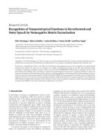
As examples, we present the orthonormal spline basis
spanning the basic spline scaling space V
0
for three degrees
4 EURASIP Journal on Advances in Signal Processing
of the spline function d = 0, d = 1, and d = 2. We star t by
providing the expression of the simplest case corresponding
to the smallest spline function degree (i.e., d
= 0). The scal-
ing basis associated to the uniform spline function of degree
d
= 0 has been initially proposed by Haar. We suggest keep-

ing the same appellation even in the irregular spaced knots.
On each bounded interval I
0,i
∈ S
0
, the basic spline space V
0
is spanned by the following scaling function:
ϕ
0
0,0,I
0,i
(t) = B
0
0,[t
i
,t
i+1
]
(t)
=
1
√
t
i+1
− t
i
for t ∈ I
0,i
,andalli ∈ N.

(18)
We concentrate now on the construction of linear ortho-
normal spline scaling basis. Among the different construc-
tion possibilities inherent to the Gram-Schmidt method, we
present the example built with the first nonuniform B-spline
function as the reference component. At any given interval
I
0,i
, the expressions of the two linear spline scaling functions
ϕ
1
0,k,I
0,i
(t) ∈ V
0
are given below:
ϕ
1
0,0,I
0,i
(t) =
√
3
t
i+1
− t

t
i+1
− t

i

3/2
,
ϕ
1
0,1,I
0,i
(t) =
3t − t
i+1
− 2t
i

t
i+1
− t
i

3/2
for t ∈ I
0,i
and all i ∈ N.
(19)
This last example concerns the quadratic orthonormal
spline scaling basis of the basic space V
0
. According to
the Gram-Schmidt method, various quadratic orthonormal
spline bases are possible. We present one construction among

others. The quadratic spline scaling functions spanning the
basic spline space V
0
are given as follows:
ϕ
2
0,0,I
0,i
(t) =
√
5

t
i+1
− t

2

t
i+1
− t
i

5/2
,
ϕ
2
0,1,I
0,i
(t) =

√
3

t
i+1
− t

5t − 4t
i
− t
i+1


t
i+1
− t
i

5/2
,
ϕ
2
0,2,I
0,i
(t) =

10t
2
−


12t
i
+8t
i+1

t +3t
2
i
+ t
2
i+1
+6t
i
t
i+1


t
i+1
− t
i

5/2
for t ∈ I
0,i
and all i ∈ N.
(20)
The orthonormal spline scaling bases given by (18), (19), and
(20)areplottedinFigure 1 on the inter val [0, 2].
3.3. Two-scale equation on irregular partition of knots

In the multiresolution traditional case, the two-scale equa-
tion plays a significant role in the design of fast orthogonal
decomposition and reconstruction algorithms. This subsec-
tion shows that even if the partition of knots is irregular, it is
possible again to obtain relationship between the spline scal-
ing functions at resolution level j and j
− 1.
The approximation spline subspace V
j−1
contains the
subspace V
j
(see (16)). So, any scaling function belonging
to V
j
, and defined on the sequence S
j
,canbedecomposed
−1
0
1
2
d = 0
00.20.40.60.81 1.21.41.61.82
(a)
−1
0
1
2
d = 1

00.20.40.60.81 1.21.41.61.82
(b)
−2
0
2
4
d = 2
00.20.40.60.81 1.21.41.61.82
(c)
Figure 1: Orthonormal spline bases for d = 0, d = 1, and d = 2.
on each bounded interval I
j,i
using the basis of the approxi-
mation subspace V
j−1
as follows:
ϕ
d
j,k,I
j,i
(t)=
1

m=0
d

n=0
h
m,n
j,k


t
2
j−1
i
, t
2
j−1
(i+1)
, t
2
j−1
(i+2)

ϕ
d
j
−1,n,I
j−1,i+m
(t)
for t
∈ I
j,i
, k ∈ [0, d], i ∈ N,
(21)
where h
m,n
j,k
represent weighted coefficients which will be
computed later.

Since
ϕ
d
j,k,I
j,i
(t), ϕ
d
j,l,I
j,p
(t)=δ
kl
δ
ip
(for all k ∈ [0, d], for
all l
∈ [0, d], for all i ∈ N and for all p ∈ N), it is easy
to show, after some manipulations, that the weighted coeffi-
cients are deduced by these equations
h
m,n
j,k

t
2
j−1
i
,t
2
j−1
(i+1)

, t
2
j−1
(i+2)

=

ϕ
d
j,k,I
j,i
(t), ϕ
d
j
−1,n,I
j−1,i+m
(t)

,
∀k ∈ [0, d], n = [0, d], m = 0, 1, i ∈ N.
(22)
In irregular knots partition, (22) proves that the filter coef-
ficients are parameterized by the positions of the knots be-
longing to the sequence S
j−1
. For writing convenience rea-
sons, these coefficients are gathered in a matrix, denoted
H
j
(t

2
j−1
i
, t
2
j−1
(i+1)
, t
2
j−1
(i+2)
) of dimension (d +1)×2(d +1),as
follows:
H
j

t
2
j−1
i
, t
2
j−1
(i+1)
, t
2
j−1
(i+2)

=

⎛
⎜
⎜
⎜
⎝
h
0,0
j,0
··· h
0,d
j,0
h
1,0
j,0
··· h
1,d
j,0
.
.
.
.
.
.
.
.
.
.
.
.
h

0,0
j,d
··· h
0,d
j,d
h
1,0
j,d
··· h
1,d
j,d
⎞
⎟
⎟
⎟
⎠
.
(23)
Anissa Zerga
¨
ınoh et al. 5
These results show that the standard filter banks are replaced
by a s et of filters depending on the position of the knots in
the sequence.
To illustrate these results, we provide the explicit expre-
ssions of the filter coefficients for three different degrees
d
= 0, d = 1, and d = 2. The approximation spline space
V
0

contains the subspace V
1
(V
1
⊂ V
0
). So, any scaling func-
tion belonging to V
1
, and defined on any bounded interval
I
1,i
∈ S
1
, can be decomposed using the basis of the approxi-
mation space V
0
. We start by the simplest case, that is, d = 0.
The Haar scaling function ϕ
0
1,0,I
1,i
(t)isthusdecomposedas
follows:
ϕ
0
1,0,I
1,i
(t) = h
0,0

1,0

t
i
, t
i+1
, t
i+2

ϕ
0
0,0,I
0,i
(t)
+ h
1,0
1,0

t
i
, t
i+1
, t
i+2

ϕ
0
0,0,I
0,i+1
(t)fort ∈ I

1,i
, i ∈ N.
(24)
The weighted coefficients
{h
0,0
1,0
(t
i
, t
i+1
, t
i+2
), h
1,0
1,0
(t
i
, t
i+1
, t
i+2
)},
computed as explained below, provides the following solu-
tions:
h
0,0
1,0

t

i
, t
i+1
, t
i+2

=
√
t
i+1
− t
i
√
t
i+2
− t
i
,
h
1,0
1,0

t
i
, t
i+1
, t
i+2

=

√
t
i+2
− t
i+1
√
t
i+2
− t
i
∀i ∈ N.
(25)
Consider now the linear spline scaling case. The decom-
position of any linear spline scaling function
{ϕ
1
1,0,I
1,i
(t),
ϕ
1
1,1,I
1,i
(t)}∈V
1
, on the basic space V
0
is expressed as a lin-
ear combination of weighted coefficients by scaling functions
{ϕ

1
0,0,I
0,i
(t), ϕ
1
0,1,I
0,i
(t), ϕ
1
0,0,I
0,i+1
(t), ϕ
1
0,1,I
0,i+1
(t)}∈V
0
as follows:
ϕ
1
1,0I
1,i
(t) = h
0,0
1,0

t
i
, t
i+1

, t
i+2

ϕ
1
0,0,I
0,i
(t)
+ h
0,1
1,0

t
i
, t
i+1
, t
i+2

ϕ
1
0,1,I
0,i
(t)
+ h
1,0
1,0

t
i

, t
i+1
, t
i+2

ϕ
1
0,0,I
0,i+1
(t)
+ h
1,1
1,0

t
i
, t
i+1
, t
i+2

ϕ
1
0,1,I
0,i+1
(t),
(26)
ϕ
1
1,1,I

1,i
(t) = h
0,0
1,1

t
i
, t
i+1
, t
i+2

ϕ
1
0,0,I
0,i
(t)
+ h
0,1
1,1

t
i
, t
i+1
, t
i+2

ϕ
1

0,1,I
0,i
(t)
+ h
1,0
1,1

t
i
, t
i+1
, t
i+2

ϕ
1
0,0,I
0,i+1
(t)
+ h
1,1
1,1

t
i
, t
i+1
, t
i+2


ϕ
1
0,1,I
0,i+1
(t).
(27)
After some appropriate manipulations (see (22)), we obtain
the following expressions for each filter coefficients:
h
0,0
1,0

t
i
, t
i+1
, t
i+2

=
(1/2)

t
i+1
− t
i

1/2

3t

i+2
− 2t
i
− t
i+1


t
i+2
− t
i

3/2
;
h
0,1
1,0

t
i
, t
i+1
, t
i+2

=

√
3/2


t
i+1
− t
i

1/2

t
i+2
− t
i+1


t
i+2
− t
i

3/2
;
h
1,0
1,0

t
i
, t
i+1
, t
i+2


=

t
i+2
− t
i+1

3/2

t
i+2
− t
i

3/2
;
h
1,1
1,0

t
i
, t
i+1
, t
i+2

= 0;
h

0,0
1,1

t
i
, t
i+1
, t
i+2

=
−

√
3/2

t
i+1
− t
i

1/2

t
i+2
− t
i+1


t

i+2
− t
i

3/2
;
h
0,1
1,1

t
i
, t
i+1
, t
i+2

=
−
(1/2)

t
i+1
− t
i

1/2

t
i+2

+2t
i
− 3t
i+1


t
i+2
− t
i

3/2
;
h
1,0
1,1

t
i
, t
i+1
, t
i+2

=
√
3

t
i+1

− t
i

t
i+2
− t
i+1

1/2

t
i+2
− t
i

3/2
;
h
1,1
1,1

t
i
, t
i+1
, t
i+2

=
√

t
i+2
− t
i+1
√
t
i+2
− t
i
∀i ∈ N.
(28)
It was shown that the more spline function degree in-
creases, the better the approximation quality of the signal is
[12]. For this reason, we are interested in high degrees al-
though the number of weighted coefficients to determine be-
comes significant. T he weighted coefficients of the quadratic
spline scaling functions
{ϕ
2
1,0,I
1,i
(t), ϕ
2
1,1,I
1,i
(t), ϕ
2
1,2,I
1,i
(t)}∈V

1
are presented at the following:
h
0,0
1,0

t
i
, t
i+1
, t
i+2

=

t
i+1
−t
i

1/2

6t
2
i
+3t
i
t
i+1
−15t

i
t
i+2
+t
2
i+1
−5t
i+1
t
i+2
+10t
2
i+2

6

t
i+2
−t
i

5/2
;
h
1,1
1,0

t
i
, t

i+1
, t
i+2

=
0;
h
0,1
1,0

t
i
, t
i+1
, t
i+2

=
√
15

t
i+1
− t
i

1/2

t
i+2

− t
i+1

2t
i+2
− t
i+1
− t
i

6

t
i+2
− t
i

5/2
;
h
0,2
1,0

t
i
, t
i+1
, t
i+2


=
√
5

t
i+1
− t
i

1/2

t
i+2
− t
i+1

3

t
i+2
− t
i

5/2
;
h
1,0
1,0

t

i
, t
i+1
, t
i+2

=

t
i+2
− t
i+1

5/2

t
i+2
− t
i

5/2
;
h
1,2
1,0

t
i
, t
i+1

, t
i+2

= 0;
h
0,0
1,1

t
i
, t
i+1
, t
i+2

=
√
15
6

t
i+1
− t
i

1/2

t
i+2
− t

i+1

t
i
+ t
i+1
− 2t
i+2


t
i+2
− t
i

5/2
;
h
0,1
1,1

t
i
, t
i+1
, t
i+2

=


t
i+1
−t
i

1/2

2t
2
i
−2t
2
i+2
+9t
i+1
t
i+2
−5t
2
i+1
−5t
i
t
i+2
+t
i
t
i+1

2


t
i+2
−t
i

5/2
;
h
0,0
1,2

t
i
, t
i+1
, t
i+2

=
√
5

t
i+2
− t
i+1

2


t
i+1
− t
i

1/2
3

t
i+2
− t
i

5/2
;
h
0,2
1,1

t
i
, t
i+1
, t
i+2

=
√
3
3


t
i+1
− t
i

1/2

t
i+2
− t
i+1

5t
i+1
− t
i+2
− 4t
i


t
i+2
− t
i

5/2
;
h
1,0

1,1

t
i
, t
i+1
, t
i+2

=
−
√
15

t
i+2
− t
i+1

3/2

t
i
− t
i+1


t
i+2
− t

i

5/2
;
h
1,1
1,1

t
i
, t
i+1
, t
i+2

=

t
i+2
− t
i+1

3/2

t
i+2
− t
i

3/2

;
h
1,2
1,1

t
i
, t
i+1
, t
i+2

= 0;
6 EURASIP Journal on Advances in Signal Processing
0
0.5
1
j
= 0
012345678
(a)
0.2
0.3
0.4
0.5
j
= 1
012345678
(b)
−1

0
1
2
j
= 2
012345678
(c)
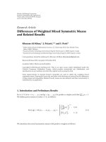
Figure 2: Haar scaling functions at resolutions j = 0, 1, 2.
h
0,1
1,2

t
i
, t
i+1
, t
i+2

=
√
3
3

t
i+2
− t
i+1

t

i+1
− t
i

1/2

t
i+2
+4t
i
− 5t
i+1


t
i+2
− t
i

5/2
;
h
0,2
1,2

t
i
, t
i+1
, t

i+2

=

t
i+1
−t
i

1/2

3t
2
i
−12t
i
t
i+1
+6t
i+2
t
i
+t
2
i+2
+10t
2
i+1
−8t
i+2

t
i+1

3

t
i+2
−t
i

5/2
;
h
1,1
1,2

t
i
, t
i+1
, t
i+2

=
√
3

t
i+1
− t

i

t
i+2
− t
i+1

1/2

t
i+2
− t
i

3/2
;
h
1,0
1,2

t
i
, t
i+1
, t
i+2

=
√
5


t
i
− t
i+1

t
i+2
− t
i+1

1/2

t
i+2
− 2t
i+1
+ t
i


t
i+2
− t
i

5/2
;
h
1,2

1,2

t
i
, t
i+1
, t
i+2

=

t
i+2
− t
i+1

1/2

t
i+2
− t
i

1/2
∀i ∈ N.
(29)
The relationships between other successive resolutions
are directly derived from the preceding solutions specified
for the resolution level j
= 1. These solutions show clearly

that the filter coefficients depend on the localization of the
sequence knots.
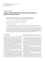
Figures 2, 3,and4 present, respectively, Haar, linear, and
quadratic spline scaling functions at three resolution levels
j
= 0, 1, 2 starting on the initial finest non-equally spaced
knots sequence S
0
= [t
0
= 0, t
1
= 2, t
2
= 4, t
3
= 7, t
4
= 8].
4. SPLINE WAVELET FUNCTION ON IRREGULAR
PARTITION OF KNOTS
This section is devoted to the construction of orthonormal
spline wavelet bases using the multiresolution specific re-
−1
0
1
2
j = 0
012345678
(a)

−0.5
0
0.5
1
j = 1
012345678
(b)
−0.5
0
0.5
1
j = 2
012345678
(c)
Figure 3: Linear scaling functions at resolutions j = 0, 1, 2.
−2
0
2
4
j = 0
012345678
(a)
−1
0
1
2
j = 1
012345678
(b)
−1

0
1
2
j = 2
012345678
(c)
Figure 4: Quadratic scaling functions at resolutions j = 0, 1, 2.
quirements in the context of irregular partition of knots.
We begin the study by int roducing the subspaces where the
spline wavelet functions live.
4.1. Spline detail subspaces
The successive approximations of a signal at two successive
resolutions j
−1and j are, respectively, obtained from the or-
thogonal projections of this signal on the respective approx-
imation subspaces V
j−1
and V
j
. The embedded structure of
Anissa Zerga
¨
ınoh et al. 7
the spline scaling subspaces involves the inclusion of the sub-
space V
j
in V
j−1
. To improve the approximated signal qual-
ity, at resolution j, one classically introduces the orthogonal

complement of V
j
in V
j−1
. This orthogonal subspace, known
as detail subspace, is denoted W
j
. Hence, the mathematical
relationship between these subspaces is as fol lows:
V
j−1
= V
j
⊕ W
j
, (30)
where the symbol
⊕ represents the direct sum between the
approximation and detail subspaces V
j
and W
j
.
This detail subspace is spanned from a set of wavelet
functions denoted ψ
d
j,k,I
j,i
(t). The dimension of the wavelet
space, on any bounded interval I

j,i
= I
j−1,i
∪ I
j−1,i+1
,isde-
duced from the previous relation as follows:
dim

W
j

=
dim

V
j−1

−
dim

V
j

∀
j ≥ 1, (31)
where dim(V
j−1
) = 2 ×(d + 1) and dim(V
j

) = d +1.
The dimension of the spline wavelet subspace is thus eas-
ily deduced and is equal to
dim

W
j

=
d +1 ∀j ≥ 1. (32)
Therefore, the detail subspace W
j
is spanned by the spline
wavelet functions defined on each bounded interval I
j,i
as
follows:
W
j
= span

ψ
d
j,k,I
j,i
(t) ∀k ∈ [0, d]; ∀j ≥ 1; ∀i ∈ N

.
(33)
4.2. Two-scale equation on irregular partition of knots

According to (30), the wavelet subspace W
j
is contained
in the approximation subspace V
j−1
. Thus, the kth wavelet
function ψ
d
j,k,I
j,i
(t), at resolution level j, can be expressed as a
linear combination of coefficients
{g
m,n
j,k
} weig hted by scaling
functions belonging to the spline subspace V
j−1
. Therefore,
on each interval I
j,i
= I
j−1,i
∪I
j−1,i+1
, we obtain the following
decomposition refereeing to the two-scale equation:
ψ
d
j,k,I

j,i
(t)=
1

m=0
d

n=0
g
m,n
j,k

t
2
j−1
i
, t
2
j−1
(i+1)
, t
2
j−1
(i+2)

ϕ
d
j
−1,n,I
j−1,i+m

(t)
with k
= 0, , d, m = 0, 1, n = 0, , d, i ∈ N.
(34)
For writing convenience reasons, the weighted coeff-
icients are also gathered in a matrix, denoted G
j
(t
2
j−1
i
,
t
2
j−1
(i+1)
, t
2
j−1
(i+2)
) of dimension (d +1)×2(d +1),asfollows:
G
j

t
2
j−1
i
, t
2

j−1
(i+1)
, t
2
j−1
(i+2)

=
⎛
⎜
⎜
⎜
⎝
g
0,0
j,0
··· g
0,d
j,0
g
1,0
j,0
··· g
1,d
j,0
.
.
.
.
.

.
.
.
.
.
.
.
g
0,0
j,d
··· g
0,d
j,d
g
1,0
j,d
··· g
1,d
j,d
⎞
⎟
⎟
⎟
⎠
.
(35)
The spline wavelet function requires the computation of
the two-scale equation coefficients
{g
m,n

j,k
}. To compute these
2(d +1)
2
coefficients, one must satisfy the conditions inher-
ent to the traditional multiresolution concept listed below.
(i) The spline scaling subspace is orthogonal to the wave-
let subspace, for any resolution level ( j
≥ 1) resulting in

ψ
d
j,k,I
j,i
(t), ϕ
d
j,l,I
j,p
(t)

=
0
with
∀k ∈ [0, d], ∀l ∈ [0, d], ∀i ∈ N, ∀p ∈ N.
(36)
(ii) The orthonorm ality conditions of the wavelet basis at all
and cross resolution levels resulting in

ψ
d

j,k,I
j,i
(t), ψ
d
j,l,I
j,p
(t)

=
δ
kl
δ
ip
with ∀k ∈ [0, d], ∀l ∈ [0, d], ∀i ∈ N, ∀p ∈ N.
(37)
These conditions gathered lead to solve the following system
of equations:
H
j

t
2
j−1
i
, t
2
j−1
(i+1)
, t
2

j−1
(i+2)

G
j

t
2
j−1
i
, t
2
j−1
(i+1)
, t
2
j−1
(i+2)

t
= 0,
G
j

t
2
j−1
i
, t
2

j−1
(i+1)
, t
2
j−1
(i+2)

G
j

t
2
j−1
i
, t
2
j−1
(i+1)
, t
2
j−1
(i+2)

t
= I
d
.
(38)
To find the 2(d +1)
2

unknown coefficients {g
m,n
j,k
},we
must find the basis of the H
j
(t
2
j−1
i
, t
2
j−1
(i+1)
, t
2
j−1
(i+2)
)null
space. The system of (38)hasd(d +1)/2 freedom degrees.
Many solutions are possible involving then the construction
of a large family of orthonormal wavelet bases. The freedom
degrees can be used judiciously to ensure some desirable fea-
tures of the wavelet functions. The system of (38) shows that
the standard filter banks are replaced by a set of filters de-
pending on the position of the knots in the sequence. Some
examples will be provided later.
4.3. Orthonormal spline wavelet basis on
bounded intervals
According to the theoretical development of the spline wave-

let bases on the irregular partition context of knots, we pro-
vide explicit expressions of the wavelet bases for three degrees
d
= 0, d = 1, and d = 2 in order to complete the required
tools of a multiresolution analysis since the scaling bases have
been already built in Section 3.
The Haar wavelet is firstly presented. Due to the struc-
ture of the multiresolution subspaces, the wavelet functions
{ψ
0
1,0,I
1,i
(t)} belonging to W
1
, can be expressed, on each
bounded interval I
1,i
= I
0,i
∪ I
0,i+1
, as follows:
ψ
0
1,0,I
1,i
(t) = g
0,0
1,0


t
i
, t
i+1
, t
i+2

ϕ
0
0,0,I
0,i
(t)
+ g
1,0
1,0

t
i
, t
i+1
, t
i+2

ϕ
0
0,0,I
0,i+1
(t).
(39)
The two weighted coefficients g

0,0
1,0
(t
i
, t
i+1
, t
i+2
), g
1,0
1,0
(t
i
, t
i+1
,
t
i+2
) are computed as previously explained. Replacing the
scaling functions by their explicit expressions, given by (19),
the generalized system of (38)becomes

t
i+1
− t
i

g
0,0
1,0


t
i
, t
i+1
, t
i+2

+

t
i+2
− t
i+1

g
1,0
1,0

t
i
, t
i+1
, t
i+2

=
0,

t

i+1
− t
i

g
0,0
1,0

t
i
, t
i+1
, t
i+2

2
+

t
i+2
− t
i+1

g
1,0
1,0

t
i
, t

i+1
, t
i+2

2
= 1.
(40)
8 EURASIP Journal on Advances in Signal Processing
−1
−0.5
0
0.5
1
j = 1
012345678
(a)
−1
−0.5
0
0.5
1
j = 2
012345678
(b)
Figure 5: Haar wavelet functions at resolution levels j = 1, 2.
Two distinct solutions are found:
g
0,0
1,0


t
i
, t
i+1
, t
i+2

=±
√
t
i+2
− t
i+1
√
t
i+2
− t
i
for t
i
≤ t<t
i+1
,
g
1,0
1,0

t
i
, t

i+1
, t
i+2

=∓
√
t
i+1
− t
i
√
t
i+2
− t
i
for t
i+1
≤ t<t
i+2
.
(41)
The relationships between successive resolutions are easily
deduced from the above equations. Figure 5 presents, at two
resolution levels j
= 1, 2, the Haar wavelet function using
one provided solution given by (41) on the finest sequence
S
0
= [t
0

= 0, t
1
= 2, t
2
= 4, t
3
= 7, t
4
= 8]. The first graph,
concerns the two wavelets functions {ψ
0
1,0,[0,3]
(t), ψ
0
1,1,[3,8]
(t)}
generating the space W
1
. The second graph represents the
wavelet function ψ
0
2,0,[0,8]
(t) spanning the space W
2
.
According to the theoretical de velopment, the linear spl-
ine wavelet functions {ψ
1
1,k,I
1,i

(t), for k = 0, 1} can be decom-
posed using the previous linear scaling basis of the space V
0
previously constructed (20) as follows:
ψ
1
1,0,I
1,i
(t) = g
0,0
1,0

t
i
, t
i+1
, t
i+2

ϕ
1
0,0,I
0,i
(t)
+ g
0,1
1,0

t
i

, t
i+1
, t
i+2

ϕ
1
0,1,I
0,i
(t)
+ g
1,0
1,0

t
i
, t
i+1
, t
i+2

ϕ
1
0,0,I
0,i+1
(t)
+ g
1,1
1,0


t
i
, t
i+1
, t
i+2

ϕ
1
0,1,I
0,i+1
,
ψ
1
1,1,I
1,i
(t) = g
0,0
1,1

t
i
, t
i+1
, t
i+2

ϕ
1
0,0,I

0,i
(t)
+ g
0,1
1,1

t
i
, t
i+1
, t
i+2

ϕ
1
0,1,I
0,i
(t)
+ g
1,0
1,1

t
i
, t
i+1
, t
i+2

ϕ

1
0,0,I
0,i+1
(t)
+ g
1,1
1,1

t
i
, t
i+1
, t
i+2

ϕ
1
0,1,I
0,i+1
(t).
(42)
The linear wavelet basis construc tion requires the computa-
tion of eight unknown coefficients
{g
m,n
1,k
(t
i
, t
i+1

, t
i+2
)}. These
coefficients are obtained by solving the equation system (38).
In the linear case, only one freedom degree is available. This
freedom degree can be used judiciously in order to impose
continuity condition of at least one wavelet function on each
knot t
2
j−1
(i+1)
inside the interval I
j,i
. For this particular case,
explicit expressions of the coefficients
{g
m,n
1,k
(t
i
, t
i+1
, t
i+2
)} are
listed below:
g
0,0
1,0


t
i
, t
i+1
, t
i+2

=
0;
g
0,1
1,0

t
i
, t
i+1
, t
i+2

=
√
t
i+2
− t
i+1
√
t
i+2
− t

i
;
g
1,0
1,0

t
i
, t
i+1
, t
i+2

=−

√
3/2

√
t
i+1
− t
i
√
t
i+2
− t
i
;
g

1,1
1,0

t
i
, t
i+1
, t
i+2

=
(1/2)
√
t
i+1
− t
i
√
t
i+2
− t
i
;
g
0,0
1,1

t
i
, t

i+1
, t
i+2

=

t
i+2
− t
i+1

3/2

t
i+2
− t
i

3/2
;
g
0,1
1,1

t
i
, t
i+1
, t
i+2


=−
√
3

t
i+2
− t
i+1

1/2

t
i+1
− t
i


t
i+2
− t
i

3/2
;
g
1,0
1,1

t

i
, t
i+1
, t
i+2

=
(1/2)

t
i+1
− t
i

1/2

4t
i+1
− 3t
i+2
− t
i


t
i+2
− t
i

3/2

;
g
1,1
1,1

t
i
, t
i+1
, t
i+2

=

√
3/2

√
t
i+1
− t
i
√
t
i+2
− t
i
.
(43)
The relationships between successive resolutions are directly

deduced from the above equations.
Figure 6 presents linear wavelet functions
{ψ
1
1,0,I
1,0
(t),
ψ
1
1,1,I
1,0
(t)} on the interval [2, 5] at resolution level j = 1,
according to four solutions (a), (b), (c), (d) depending on the
freedom degree of the equation system (38). Among these
solutions, the graphs (a) show that the continuity of one
wavelet function ψ
1
1,1,I
1,0
(t) is ensured at the knot t
1
= 3.
Figure 7 presents the linear wavelet bases at two resolution
levels j
= 1, 2 on the initial finest sequence S
0
= [t
0
= 0, t
1

=
2, t
2
= 4, t
3
= 7, t
4
= 8].
The quadratic spline wavelet functions {ψ
2
1,k,I
1,i
(t), for
k
= 0, 1, 2} can be decomposed using the basis of the ap-
proximation space V
0
as follows:
ψ
2
1,k,I
1,i
(t)
=
1

m=0
2

n=0

g
m,n
1,k

t
i
, t
i+1
, t
i+2

ϕ
2
0,n,I
0,i
(t)
+
1

m=0
2

n=0
g
m,n
1,k

t
i
, t

i+1
, t
i+2

ϕ
2
0,n,I
0,i+1
(t)fork = 0, 1, 2.
(44)
Anissa Zerga
¨
ınoh et al. 9
−2
0
2
j = 1
0345
−2
0
2
j = 1
2345
(a)
−2
0
2
j = 1
0345
−2

0
2
j = 1
2345
(b)
−2
0
2
j = 1
0345
−2
0
2
j = 1
2345
(c)
−2
0
2
j = 1
0345
−2
0
2
j = 1
2345
(d)
Figure 6: Four orthonormal linear wavelet bases at resolution level j = 1.
−2
−1

0
1
j = 1
02468
−1
0
1
2
j = 1
02468
(a)
−1
−0.5
0
0.5
1
j = 2
02468
−1
−0.5
0
0.5
1
1.5
j = 2
0123
(b)
Figure 7: Linear wavelet functions at resolution levels j = 1, 2.
−2
−1

0
1
0123 456
(a)
−2
−1
0
1
0123 456
(b)
−2
−1
0
1
0123 456
(c)
Figure 8: Orthonormal quadratic wavelet basis (no particular con-
ditions).
−2
−1
0
1
0123 456
(a)
−2
−1
0
1
0123 456
(b)

−2
−1
0
1
0123 456
(c)
Figure 9: Orthonormal quadratic wavelet basis (one continuity
condition).
10 EURASIP Journal on Advances in Signal Processing
−2
−1
0
1
0123 456
(a)
−1
−0.5
0
0.5
0123 456
(b)
−1
0
1
2
0123 456
(c)
Figure 10: Orthonormal quadratic wavelet basis (two continuity
conditions).
The 18 unknown coefficients {g

m,n
1,k
(t
i
, t
i+1
, t
i+2
), for m =
0, 1; n = 0, 1, 2 and k = 0, 1, 2} are deduced from the reso-
lution of the equation system (38) which has three freedom
degrees. The graphs of Figure 8 present an example of or-
thonormal quadratic spline wavelet basis at resolution level
j
= 1 on the initial sequence S
0
= [0, 2, 6]. No particular con-
dition is imposed to these wavelet functions while in Figure 9
only one freedom degree is exploited to ensure the continuity
of the first wavelet function on the bounded interval [0, 6], at
the knot 2. Figure 10 uses two freedom degrees to ensure the
continuity of the first and second wavelet functions.
5. ORTHOGONAL DECOMPOSITION
AND RECONSTRUCTION
This section concerns the orthogonal decomposition of a
given signal f (t) using the scaling and wavelet functions pre-
sented in the previous section. At any resolution level j
− 1,
the approximation of the signal f (t) on the spline subspace
V

j−1
on the interval I
j−1,i
,isdenotedas f
j−1,I
j−1,i
(t). Start-
ing with the orthogonally property of the scaling and wavelet
subspaces (V
j−1
= V
j
⊕ W
j
), one can decompose the signal
f
j−1,I
j−1,i
(t) ∈ V
j−1
, on each interval I
j−1,i
, according to the
following relation:
f
j−1,I
j−1,i
(t) = f
j,I
j,i

(t)+r
j,I
j,i
(t)fori ∈ N, j>1, (45)
where r
j,I
j,i
(t) is the detail signal at resolution le vel j.
Since the approximation signal f
j,I
j,i
(t)(resp.,r
j,I
j,i
(t)) be-
longs to V
j
(resp., W
j
) the function can be expressed as
a linear weighted combination of the functions belonging
to V
j
(resp., W
j
). Thus, the approximation of the signal
f
j−1,I
j−1,i
(t) ∈ V

j−1
becomes
f
j−1,I
j−1,i
(t) =
2i+1

m=2i
1

k=0
c
m
j,k
ϕ
d
j,k,I
j,m
(t)
+
2i+1

m=2i
1

k=0
d
m
j,k

ψ
d
j,k,I
j,m
(t) ∀i ∈ N,
(46)
where the weighted coefficients
{c
m
j,k
} (resp., {d
m
j,k
})aregiven
by the orthogonal projection of f
j,I
j,i
(t)(resp.,r
j,I
j,i
(t)) on the
approximation subspace V
j
(resp., W
j
). After some manip-
ulations, we show that these coefficients
{c
m
j,k

} are closely re-
lated to
{c
l
j
−1,k
} and {h
l,n
j,k
}, on the bounded interval I
j,i
,as
follows:
c
m
j,k
=
2i+1

l=2i
1

n=0
h
l,n
j,k
c
l
j
−1,k

for k = 0, 1; m = 2i,2i +1;
and all i
∈ N.
(47)
This expression can be written in a matrix form as follows:
c
j,I
j,i
= H
j,I
j,i
c
j−1,I
j,i
, (48)
where
c
j,I
j,i
=

c
2i
j
−1,0
c
2i
j
−1,1
c

2i+1
j
−1,0
c
2i+1
j
−1,1

t
,
c
j−1,I
j,i
=

c
i
j
−1,0
c
i
j
−1,1

t
,
H
j,I
j,i
=

⎛
⎜
⎝
h
2i,0
j,0
h
2i,1
j,0
h
2i+1,0
j,0
h
2i+1,1
j,0
h
2i,0
j,1
h
2i,1
j,1
h
2i+1,0
j,1
h
2i+1,1
j,1
⎞
⎟
⎠

.
(49)
The matrix H
j,I
j,i
is then easily generalized to the complete
sequence
S
j
: H
j
=
⎡
⎢
⎢
⎢
⎢
⎢
⎢
⎣
H
j,I
j,0
[0] [0] [0]
[0] H
j,I
j,1
[0]
.
.

.
.
.
.[0]
.
.
.
[0]
[0] [0] [0] H
j,I
j,n
⎤
⎥
⎥
⎥
⎥
⎥
⎥
⎦
. (50)
Thepreviousequationrelativetotheboundedintervalbe-
comes
c
j
= H
j
c
j−1
where c
j

=

c
j,I
j,0
c
j,I
j,1
···

t
,
c
j−1
=

c
j−1,I
j−1,0
c
j−1,I
j−1,2
···

t
.
(51)
Anissa Zerga
¨
ınoh et al. 11

−32
−30
−28
−26
−24
−22
−20
−18
−16
−14
0.50.52 0.54 0.56 0.58 0.60.62 0.64 0.66 0.68
Figure 11: Original signal irregularly subsampled.
The details coefficients, after some manipulations, satisfy the
following equation:
d
m
j,k
=
2i+1

l=2i
1

n=0
g
l,n
j,k
c
l
j

−1,k
for k = 0, 1; m = 2i,2i +1;
and all i
∈ N.
(52)
Using the same notation as the matrix decomposition H
j,I
j,i
,
the computation of the detail coefficients at resolution j,on
the bounded inter val I
j,i
, are given as follows:
d
j,I
j,i
= G
j,I
j,i
c
j−1,I
j,i
where d
j−1,I
j,i
=

d
i
j

−1,0
d
i
j
−1,1

t
,
G
j,I
j,i
=
⎛
⎝
g
2i,0
j,0
g
2i,1
j,0
g
2i+1,0
j,0
g
2i+1,1
j,0
g
2i,0
j,1
g

2i,1
j,1
g
2i+1,0
j,1
g
2i+1,1
j,1
⎞
⎠
.
(53)
The extension of the matrix decomposition G
j,I
j,i
to the se-
quence S
j
is obviously deduced as H
j,I
j,i
. Since the decompo-
sition is orthogonal, the reconstruction matrices are deduced
from the decomposition matrices. The decomposition matri-
ces H
j
and G
j
are sparse matrices. Therefore, the decompo-
sition and reconstruction steps will be efficient since efficient

algorithms for multiplying a sparse matrix with a vector ex-
ist.
Simulation results of the theoretical orthogonal decom-
position are provided below. The curve in Figure 11 presents
the original signal irregularly subsampled on which the pro-
vided simulations are carried out. The samples of the sig-
nal are marked by the symbol “
◦.” Figure 12 presents ap-
proximation signals (left graphs of (a), (b), (c), (d), and (e))
and detail signals (right graphs of (a), (b), (c), (d), and (e))
corresponding to five resolution levels j
= 1, 2, 3, 4, 5 us-
ing Haar wavelet and scaling functions given in Sections 3
and 4. For each graphs plotted in (a), (b), (c), (d), and (e),
the following symbols “
◦,” “ ∗,” and “+” represent, respec-
tively, (i) the subsampled data corresponding to the knots
of the sequence S
j
, (ii) the approximation signals at differ-
ent resolution level j and (iii) the detail signals at different
resolution level j. Simulation results show that, while be-
ing in the framework of irregularly spaced data, the behavior
of the multiresolution analysis is exactly the same as in the
traditional case (regularly spaced data). One can notice that
the detail signal variance is smaller than the approximation
signal variance. Moreover, the computations show that the
detail signal variances increase when going from resolution
level j
− 1toj.

6. CONCLUSION
The main objective of this paper is to provide the required
tools for achieving a multiresolution analysis in the specific
context of irregularly spaced data. In this environment, the
presented work shows that the construction of orthonormal
spline scaling and wavelet bases remains always possible. The
construction of the bases is carried out in the multiresolution
concept exploiting the orthogonal decomposition approach.
The basic tool of this paper is the nonuniform B-spline
function. This function presents many interesting properties
such as explicit and generalized expression whatever the de-
gree of the spline function when imposing a particular mul-
tiplicity on each knot of the initial sequence. In this case, the
support of the B-spline is reduced to two consecutive knots
in the sequence.
The orthonormalization process of the basic spline ba-
sis is performed with the classical Gram-Schmidt method
on each bounded intervals of the initial sequence. The pa-
per provided a genera lization of the orthonormal spline scal-
ing and wavelet bases construction whatever the degree of
the spline function. Our study proves that the scaling and
wavelet functions are not, respectively, given by dilating and
translating a unique prototype function as in the traditional
case. The traditional filter banks are replaced by a set of filters
depending on the localization of the samples in the sequence.
When the degree of the spline function increases, the number
of freedom degrees increase offering thus flexibility in the de-
sign of the wavelet functions. It is possible to ensure desirable
features such as the continuity of the wavelet function and its
successive derivatives. The complete process of decomposing

and reconstructing a signal irregularly sampled is provided.
The orthogonal decomposition, applied to signals irregularly
subsampled, shows that the traditional multiresolution anal-
ysis behaviour is respected.
Increasing the degree of the spline function allows cir-
cumventing the discontinuity problem of the scaling and
wavelet functions at the cost of a very high computational
complexity. The number of the scaling and wavelet functions
to handle becomes very high. Consequently in future inves-
tigation, a great importance will be attached to this crucial
problem.
A generalization of the proposed method to the two-
dimensional wavelet transform will be studied. The problems
involved in the topic of data compression using nonuniform
scaling and wavelet functions are interesting to be considered
in future investigations.
12 EURASIP Journal on Advances in Signal Processing
−32
−30
−28
−26
−24
−22
−20
−18
−16
−14
j = 1
0.50.54 0.58 0.62 0.66
(a)

−2
−1
0
1
2
3
4
5
6
j = 1
0.50.54 0.58 0.62 0.66
(b)
−32
−30
−28
−26
−24
−22
−20
−18
−16
−14
j = 2
0.50.54 0.58 0.62 0.66
(c)
−2
−1
0
1
2

3
4
5
6
j = 2
0.50.54 0.58 0.62 0.66
(d)
−32
−30
−28
−26
−24
−22
−20
−18
−16
−14
j = 3
0.50.54 0.58 0.62 0.66
(e)
−2
−1
0
1
2
3
4
5
6
j = 3

0.50.54 0.58 0.62 0.66
(f)
−30
−28
−26
−24
−22
−20
−18
−16
j = 4
0.50.54 0.58 0.62 0.66
(g)
−2
−1
0
1
2
3
4
5
6
j = 4
0.50.54 0.58 0.62 0.66
(h)
−32
−30
−28
−26
−24

−22
−20
−18
−16
−14
j = 5
0.50.54 0.58 0.62 0.66
(i)
−2
−1
0
1
2
3
4
5
6
j = 5
0.50.54 0.58 0.62 0.66
(j)
Figure 12: Multiresolution analysis on five resolution levels using Haar scaling and wavelet functions.
Anissa Zerga
¨
ınoh et al. 13
ACKNOWLEDGMENT
The authors would like to thank Professor Pierre Duhamel
for many interesting and helpful discussions.
REFERENCES
[1] S. Mallat, A Wavelet Tour of Signal Processing, Academic Press,
San Diego, Calif, USA, 2nd edition, 1999.

[2] M. Vetterli and J. Kovacevic, Wavelets and Subband Coding,
Prentice Hall, Englewood Cliffs, NJ, USA, 1995.
[3] C.K.Chui,Ed.,Wavelets: A Tutorial in Theory and Applica-
tions, Academic Press, San Diego, Calif, USA, 1993.
[4] O. Rioul and P. Duhamel, “Fast algorithms for wavelet
transform computation,” in Time-Frequency and Wavelets in
Biomedical Signal Processing, M. Akay, Ed., chapter 8, pp. 211–
242, Wiley-IEEE Press, New York, NY, USA, 1997.
[5] M. D. Buhmann and C. A. Micchelli, “Spline prewavelets for
non-uniform knots,” Numerische Mathematik,vol.61,no.1,
pp. 455–474, 1992.
[6] I. Daubechies, I. Guskov, P. Schr
¨
oder, and W. Sweldens,
“Wavelets on irregular point sets,” Philosophical Transactions
of the Royal Society of London. A, vol. 357, no. 1760, pp. 2397–
2413, 1999.
[7] I. Daubechies, I. Guskov, and W. Sweldens, “Commutation
for irregular subdivision,” Constructive Approximation, vol. 17,
no. 4, pp. 479–514, 2001.
[8] T. Lyche, K. Mørken, and E. Quak, “Theory and Algorithms
for non-uniform spline wavelets,” in Multivariate Approxima-
tion and Applications, N. Dyn, D. Leviatan, D. Levin, and A.
Pinkus, Eds., pp. 152–187, Cambridge University Press, Cam-
bridge, UK, 2001.
[9] C. De Boor, A Practical Guide to Splines, Springer, New York,
NY, USA, revised edition, 2001.
[10] G. Farin, Curves and Surfaces for CAGD, Morgan-Kaufmann,
San Fransisco, Calif, USA, 5th edition, 2001.
[11] N. Chihab, A. Zerga

¨
ınoh, P. Duhamel, and J. P. Astruc, “The
influence of the non-uniform spline basis on the approxima-
tion signal,” in Proceedings of 12th European Signal Processing
Conference (EUSIPCO ’04), Vienna, Austria, September 2004.
[12] M. A. Unser, “Ten good reasons for using spline wavelets,”
in Wavelet Applications in Signal and Image Processing V,
vol. 3169 of Proceedings of SPIE, pp. 422–431, San Diego, Calif,
USA, July 1997.
Anissa Zerga
¨
ınoh received the State En-
gineering degree in electrical engineering
from National Telecommunication School
in 1989, the M.S. degree in information
technology in 1990, and the Ph.D. degree
in 1994 all from University Paris 11, Or-
say, France. From 1992 to 1994, she worked
at the National Institute of Telecommunica-
tions (INT, Evry, France) where her research
activities were on digital signal processing,
fast filtering algorithms, and implementation problems on DSP.
Since 1997, she is Associate Professor at Galil
´
ee Institute of Univer-
sity Paris 13, France. From 2005 to 2007, she joined the CNRS/LSS
laboratory, Sup
´
elec, Orsay, France as a Visiting Professor. Her cur-
rent research interests include image and video compression, im-

age reconstruction, irregular sampling, interpolation, and wavelet
transforms.
Najat Chihab received her M.S. degree
in information technology from University
Paris 11, France in 2001. She received the
Ph.D. degree from the University Paris 13,
France in 2005. Her research interests fo-
cus on nonuniform B-spline function, in-
terpolation, approximation, irregular sub-
sampling, and multiresolution analysis.
Jean Pierre Astruc was born in France in
1953. He received the Dr.Ing. degree in
1979 and the Doctorat es Sciences degree
in physics in 1987 both at University Paris
13, France. His first research interests were
in the energy transfer between atoms and
molecules. Since 1992, he is Professor at
University Paris 13, France. From 1988 to
1998 he founded a working group of expe-
rience’s control in the LIMHP/CNRS Lab-
oratory at University Paris 13, France. His research activities were
concentrated on the measurements of the critical parameters of a
pure fluid by expert system and on the experiments control using
image processing. He joined the L2TI Laboratory of Galil
´
ee Insti-
tute, University Paris 13 in 1998. Since 2002, he is the Head of the
Galil
´
ee Institute. His current research interests include image and

video compression.