Báo cáo hóa học: " Research Article Inverse Filtering for Speech Dereverberation Less Sensitive to Noise and Room Transfer Function Fluctuations" potx

Hindawi Publishing Corporation
EURASIP Journal on Advances in Signal Processing
Volume 2007, Article ID 34013, 12 pages
doi:10.1155/2007/34013
Research Article
Inverse Filtering for Speech Dereverberation Less Sensitive to
Noise and Room Transfer Function Fluc tuations
Tak afumi Hikichi, Marc Delcroix, and Masato Miyoshi
Media Information Laboratory, NTT Communication Science Laboratories, NTT Corporation, 2-4 Hikaridai, Seika-cho,
Soraku-gun, Kyoto 619-0237, Japan
Received 16 November 2006; Accepted 2 February 2007
Recommended by Liang-Gee Chen
Inverse filtering of room transfer functions (RTFs) is considered an attractive approach for speech dereverberation given that the
time invariance assumption of the used RTFs holds. However, in a realistic environment, this assumption is not necessarily guar-
anteed, and the performance is degraded because the RTFs fluctuate over time and the inverse filter fails to remove the effectofthe
RTFs. The inverse filter may amplify a small fluctuation in the RTFs and may cause large distortions in the filter’s output. Moreover,
when interference noise is present at the microphones, the filter may also amplify the noise. This paper proposes a design strategy
for the inverse filter that is less sensitive to such disturbances. We consider that reducing the filter energy is the key to making
the filter less sensitive to the disturbances. Using this idea as a basis, we focus on the influence of three design parameters on the
filter energy and the performance, namely, the regularization parameter, modeling delay, and filter length. By adjusting these three
design parameters, we confirm that the performance can be improved in the presence of RTF fluctuations and interference noise.
Copyright © 2007 Takafumi Hikichi et al. This is an open access article distributed under the Creative Commons Attribution
License, which permits unrestricted use, distribution, and reproduction in any medium, provided the original work is properly
cited.
1. INTRODUCTION
Inverse filtering of room acoustics is useful in various ap-
plications such as sound reproduction, sound-field equal-
ization, and speech dereverberation. Usually, room trans-
fer functions (RTFs) are modeled as finite impulse response
(FIR) filters, and inverse filters are designed to remove the
effect of the RTFs. When the RTFs are known apriorior

are capable of being accurately estimated, this approach has
been shown to achieve high inverse filtering performance [1–
4]. However, in actual acoustic environments, there are dis-
turbances that affect the inverse fi ltering performance. One
cause of these disturbances is the fluctuation in the RTFs re-
sulting from changes in such factors as source position and
temperature [5–9]. As a result, an inverse filter correctly de-
signed for one condition may not work well for another con-
dition, and compensation or adaptation processing may be-
come necessary.
The sensitivity issue with inverse filtering in relation to
the movement of a sound source or microphone has been
addressed in se veral papers. In [8, 9], the sensitivity of in-
verse filters is quantified in terms of the mean-squared error
(MSE), defined as the power of the deviation of the equal-
ized impulse response from the ideal impulse. This MSE
is theoretically derived based on statistical room acoustics.
These studies claim that the region in which the MSE is be-
low
−10 dB is restricted to a few tenths of a wavelength of a
target signal, revealing a high sensitivity to small positional
changes. That is, when an inverse filter designed for a cer-
tain location is applied to recover signals observed at another
location, the performance easily degrades and the MSE be-
comes high.
Inverse filters are usually obtained by inverting the
autocorrelation matrix of the RTFs. Accordingly, in order to
realize stable inverse filtering, either regularization [10]or
the truncated singular value decomposition method [11–13]
has been applied. With the latter method, the small singular

values of the autocorrelation matrix of the RTFs are treated
as zeros. Both methods have been applied to a sound repro-
duction system, and have been experimentally verified.
The purpose of this paper is to pursue ways of designing
inverse filters that are less sensitive to RTF fluctuations and
interference noise. When the RTFs fluctuate, the inverse fil-
ter may amplify the small fluctuation in the RTFs and may
cause large distortions in the output signal of the inverse fil-
ter. Moreover, when the microphone signal contains noise,
2 EURASIP Journal on Advances in Sig nal Processing
x
1
(n)
.
.
.
x
P
(n)
s(n)
Speaker
.
.
.
H
1
(z)
H
P
(z)

Room soundfield
Mic.
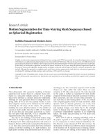
Figure 1: Single-source multimicrophone acoustic system. H
i
(z)
represent room transfer functions.
the inverse filter may also amplify the noise. We expect the
filtered signal to be less degraded when the filter energy is
small. Hence, we believe that reducing the filter energy is the
key to making the filters less sensitive. To confirm this belief,
we focus on the influence of three parameters used in the
design of inverse filters: the regularization parameter, filter
length, and modeling delay. By selecting proper parameter
values, we expect to reduce the filter energy, and hence make
the filter more robust to RTF variations and noise.
The organization of this paper is as follows. The follow-
ing section describes the acoustic system with a single source
and multiple microphones considered in this paper. It then
describes how inverse filters are calculated and a nalyzes the
effect of the three design parameters on the filter energy.
Section 3 reports experiments undertaken in the presence
of noise. Section 4 describes experimental results for an in-
verse filter with RTF fluctuations caused by source position
changes. Section 5 provides an analysis of the RTF fluctua-
tions caused by source p osition changes. Section 6 concludes
the paper.
2. PROBLEM FORMULATION
2.1. Acoustic system in consideration
We consider an acoustic system with a single sound source
and multiple microphones as shown in Figure 1. The source

signal is represented as s(n), where n denotes a discrete
time index, and the signals received by the microphones are
x
i
(n), i = 1, , P,whereP is the number of microphones.
Microphone signals x
i
(n)aregivenby
x
i
(n) = h
i
(n) ∗ s(n)+w
i
(n)(1)
=
J

k=0
h
i
(k)s(n − k)+w
i
(n), i = 1, , P,(2)
where
∗ denotes the convolution operation, h
i
(k), k =
0, , J, denotes the room impulse response between the
source and the ith microphone, and w

i
(n) denotes noise. The
RTFs are expressed as
H
i
(z) =
J

k=0
h
i
(k)z
−k
, i = 1, , P. (3)
We assume hereafter that these RTFs have no common zeros
among all the channels.
Equation (2) can be expressed in a matrix form as
x(n)
= H
T
s(n)+w(n), (4)
where
x(n)
=
⎡
⎢
⎢
⎣
x
1

(n)
.
.
.
x
P
(n)
⎤
⎥
⎥
⎦
, x
i
(n)=
⎡
⎢
⎢
⎢
⎢
⎣
x
i
(n)
x
i
(n − 1)
.
.
.
x

i
(n − M +1)
⎤
⎥
⎥
⎥
⎥
⎦
, i=1, , P,
w(n)
=
⎡
⎢
⎢
⎣
w
1
(n)
.
.
.
w
P
(n)
⎤
⎥
⎥
⎦
, w
i

(n)=
⎡
⎢
⎢
⎢
⎢
⎣
w
i
(n)
w
i
(n − 1)
.
.
.
w
i
(n − M +1)
⎤
⎥
⎥
⎥
⎥
⎦
, i = 1, , P,
s(n)
=
⎡
⎢

⎢
⎢
⎢
⎣
s(n)
s(n
− 1)
.
.
.
s(n
− J − M +1)
⎤
⎥
⎥
⎥
⎥
⎦
,
H
=

H
1
, , H
P

,
H
i

=
⎛
⎜
⎜
⎜
⎜
⎜
⎜
⎜
⎜
⎜
⎜
⎜
⎜
⎜
⎜
⎜
⎝
h
i
(0) 0 0
h
i
(1) h
i
(0)
.
.
.
.

.
.
.
.
. h
i
(1)
.
.
.
0
h
i
(J)
.
.
.
.
.
.
h
i
(0)
0 h
i
(J) h
i
(1)
.
.

.
.
.
.
.
.
.
.
.
.
0 0 h
i
(J)
⎞
⎟
⎟
⎟
⎟
⎟
⎟
⎟
⎟
⎟
⎟
⎟
⎟
⎟
⎟
⎟
⎠

⎫
⎪
⎪
⎪
⎪
⎪
⎪
⎪
⎪
⎪
⎪
⎪
⎪
⎪
⎪
⎪
⎪
⎬
⎪
⎪
⎪
⎪
⎪
⎪
⎪
⎪
⎪
⎪
⎪
⎪

⎪
⎪
⎪
⎪
⎭

 
M
(J + M),
(5)
and M is the block size of the microphone signals for each
channel. The objective of dereverberation is to recover source
signal s(n) from the received signal x(n). This is achieved by
filtering the received signal with the inverse filter of room
acoustic system H.
2.2. Inverse filter calculation
Generally, the inverse filter vector, denoted as g, is calculated
by minimizing the following cost function:
C
=Hg − v
2
,(6)
where
a denotes the l
2
-norm of vector a,where
g =

g
1

(1), , g
1
(M), , g
P
(1), , g
P
(M)
  
PM

T
,
v
= [0, ,0
  
d
,1,0, ,0]
T
,
(7)
M is the filter length for each channel, and d (0
≤ d ≤ PM)
is the modeling delay [14]. Here, modeling delay can be se-
lected arbitrarily. By applying this inverse filter g to the mi-
crophone signals, the filter’s output signal is equivalent to the
Takafumi Hikichi et al. 3
input signal delayed by d-taps. Hereafter, we consider that
impulse responses h
i
(n) are normalized by their norm. When

RTF matrix H is given, such inverse filter set can be calculated
as
g
= H
+
v,(8)
where A
+
is the Moore-Penrose pseudoinverse of matrix A
[15]. The inverse filter set is calculated based on the multiple-
input/output inverse theorem (MINT) [1]. The filter set with
minimum length is obtained by setting M so that matrix H
is square, which leads to M
= M
min
= J/(P − 1). The filter
length can be set at M>J/(P
− 1) as well.
2.3. Inverse filters with disturbances
When noise is present at the microphones, distortion occurs
in the output signal of the inverse filter. The larger the filter
energy is, the larger the distortion can be. Thus, we introduce
the filter energy into the cost function expressed in (6). By
taking the filter energy into consideration, the cost function
is modified as follows:
C
=Hg − v
2
+ δg
2

,(9)
where δ(
≥ 0) is a scalar variable. This parameter determines
how much weight to assign to the energy term, and thus
determines a tradeoff between the filter’s accuracy and the
amount of distortion. The same formulation is applied as
the one used in multichannel active noise control systems
[14, 16]. We would like to derive a solution that minimizes
this cost f unction. Equation ( 9)canberewrittenas
C
= (Hg − v)
T
(Hg − v)+δg
T
g
= g
T
H
T
Hg − g
T
H
T
v − v
T
Hg + v
T
v + δg
T
g.

(10)
By taking derivatives with respect to g and setting them equal
to zero, the following solution is derived:
g
r
=

H
T
H + δI

−1
H
T
v, (11)
where I is an identity matrix. T his solution has a similar
form to that of Tikhonov regularization for ill-posed prob-
lems [11–13, 17]. We hereafter refer to δ as a regularization
parameter, and g
r
as an inverse filter vector with regulariza-
tion.
Equation (11) is an optimum solution when the interfer-
ence noise is white noise with small variance δ, and the term
δI corresponds to the correlation matrix of the noise. If the
colored noise is considered as a more general case, its corre-
lation matrix is replaced with term δI as
g
r
=


H
T
H + R
n

−1
H
T
v, (12)
where R
n
is the noise correlation matrix.
Then, let us consider the situation where RTFs fluctu-
ate. Suppose fluctuated RTFs denoted as
H +

H,whereH
and

H represent the mean RTF and the fluctuation from the
mean RTF, respectively. In this case, we consider the ensem-
ble mean of the total squared error,
C
= E



(H +


H)g − v


2

=
E

(Hg − v +

Hg)
T
(Hg − v +

Hg)

=
(Hg − v)
T
(Hg − v)
+ E

(Hg − v)
T

Hg +(

Hg)
T
(Hg − v)+g

T

H
T

Hg

=
g
T
H
T
Hg − g
T
H
T
v − v
T
Hg + v
T
v + g
T
E


H
T

H


g,
(13)
where E
· represents the expectation operation. In this
derivation, we assume E


H is a zero matrix. Then, the fol-
lowing filter minimizes the cost func tion expressed in (13):
g
r
=

H
T
H + R
H

−1
H
T
v, (14)
where R
H
= E

H
T

H. From discussions described above, we

can treat the disturbances by using the filter expressed in the
following form:
g
r
=

H
T
H + R

−1
H
T
v, (15)
where H is either H or the mean RTF
H,andR is the cor-
relation matrix of either the noise R
n
or the fluctuation R
H
.
If the fluctuation could be regarded as white noise, R
= δI
could be applied to the inverse filter. In the following experi-
ments, we investigate the performance of the inverse fi lter of
the form
g
r
=


H
T
H + δI

−1
H
T
v, (16)
where
H
=
⎧
⎨
⎩
H (noise case),
H (fluctuation case).
(17)
2.4. Influence of design parameters on filter energy
Regularization parameter δ increases the minimum eigen-
value of matrix (H
T
H + δI)in(16), and hence reduces the
norm of the inverse filter. Increasing the regularization pa-
rameter is thus believed to reduce the sensitivity to RTF var i-
ations and noise. On the other hand, increasing this param-
eter reduces the accuracy of the inverse filter with respect to
the true RTFs.
The effect of the filter length can be expected as follows.
Equation (16) will give the minimum norm filter for a given
length M. By increasing the filter length, we compare var-

ious filters with different lengths, and consequently expect
that the filter with the smallest norm can be found.
A modeling delay d is also used to make the inverse filter
stable. When a nonzero modeling delay d (d
≥ 1) is used, we
also expect the filter norm to be reduced because the causal-
ity constraint is relaxed. The filter may correspond to the
minimum-norm solution that could be obtained in the fre-
quency domain [18].
As described above, we can expect the regularization pa-
rameter, filter length, and modeling delay to be effective in
reducing the filter energy.
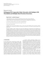
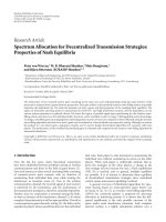
4 EURASIP Journal on Advances in Sig nal Processing
• Room height: 250 cm
• Microphone height: 100 cm
• Loudspeaker height: 150 cm
M4
M3
M2
M1
20 cm
20 cm
20 cm
100 cm100 cm
100 cm 100 cm
445 cm
355 cm
Microphone
Loudspeaker
Figure 2: Source and microphone arrangement. M1, M2, M3, and

M4 denote the microphones.
3. EXPERIMENTS ON THE EFFECT OF NOISE
Experiments were performed to verify the effectiveness of our
strategy in the presence of additive white noise.
3.1. Experimental setup
Figure 2 shows the arrangement of the source and the micro-
phones used in the experiment. Four microphones are used
(P
= 4), and room impulse responses between the source and
the microphones are simulated by using the image method
[19]. The sampling frequency is set at 8 kHz. The impulse
responses are truncated to 4000 samples (J
= 3999), corre-
sponding to
−60 dB attenuation (the reverberation time of
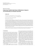
the room is 500 ms). Figure 3 shows an example of the im-
pulse response and its frequency response.
We define the input and output SNRs as follows. For the
ith microphone, the input SNR is defined as
SNR
in
= 10 log
10


N
n=0
y
2
i

(n)

N
n=0
w
2
i
(n)

, (18)
where y
i
(n) is the reverberant signal without noise, and w
i
(n)
is the noise. In the experiment, we adjust the input SNR by
controlling the amplitude of the noise signal. The output
SNRisdefinedas
SNR
out
= 10 log
10


N
n=0

y(n)
T
g

r

2

N
n
=0

w(n)
T
g
r

2

, (19)
where y(n)
= H
T
s(n) is the reverberant signal vector. This
output SNR is obtained by filtering the reverberant and the
noise s ignals separately and taking the power ratio of the
output signals.
−0.2
0
0.2
0.4
0.6
Amplitude
0 100 200 300 400 500

Time (ms)
−30
−20
−10
0
10
Magnitude (dB)
0 500 1000 1500 2000 2500 3000 3500 4000
Frequency (Hz)
Figure 3: Waveform of a room impulse response h
1
(n) and its fre-
quency characteristics.
3.2. Evaluation criteria
In order to avoid any dependency of the results on the source
signal, we used uncorrelated white signals with a duration of
3 seconds for both source signal and noise rather than speech.
The dereverberation performance is evaluated by using
the signal-to-distortion ratio (SDR) defined as
SDR
= 10 log
10


N
n
=0
s
2
(n)


N
n=0

s(n) − s(n)

2

, (20)
where s(n) is the original source signal and
s(n) is the output
signal of the inverse filter defined as
s(n) = x(n)
T
g
r
.
3.3. Results
Figure 4 shows the filter energy with various modeling de-
lays and regularization parameters when the minimum filter
length M
= M
min
= 1333 is used, as described in Section 2.2.
The energy decreases with increases in both the modeling de-
lay a nd the regularization parameter, and shows the mini-
mum value when δ
= 10
−1
and d = 500.

Figure 5 shows the inverse filter calculated with δ
= 10
−6
and δ = 10
−1
when the modeling delay is fixed at d = 500.
We clearly observed that the filter energy was reduced by in-
creasing the regular ization parameter.
Figure 6 shows the performance of the inverse filter with
an input SNR of 20 dB. We observed that a proper regular-
ization parameter value of δ
= 10
−2
gives the largest SDR
for all the modeling delay values. This regularization param-
eter corresponds to the input SNR (20 dB). When the regu-
larization parameter is smaller than 10
−2
, the performance
monotonically decreased as the regularization parameter de-
creased, according to the increase in the filter energy. Even
though the filter norm decreases with δ
= 10
−1
, the per-
formance also deteriorated because the accuracy of the filter
Takafumi Hikichi et al. 5
0
1
2

3
4
5
6
7
8
Filter energy
10
−9
10
−4
10
−3
10
−2
10
−1
Regularization parameter
d
= 0
d
= 100
d
= 200
d
= 300
d
= 400
d
= 500

Figure 4: Filter energy as a function of regularization parameter
and modeling delay (filter length is fixed at M
= 1333).
−0.2
−0.1
0
0.1
0.2
0 200 400 600 800 1000 1200
(a)
−0.2
−0.1
0
0.1
0.2
0 200 400 600 800 1000 1200
(b)
Figure 5: An example of inverse filter g
1
(n) calculated with δ =
10
−6
(a) and δ = 10
−1
(b) (modeling delay is fixed at d = 500).
decreased and the deviation of the equalized response from
the ideal one became large.
In the second experiment, the modeling delay was fixed
at d
= 500, and the effect of filter length M was investigated

with various regularization parameters δ. Figures 7 and 8
show the filter energy and corresponding performance in this
case. In Figure 7, the energy decreases with increases in both
the filter length and the regularization parameter, although
the effect of the filter length is less significant when a large
0
5
10
15
20
25
SDR (dB)
10
−9
10
−4
10
−3
10
−2
10
−1
Regularization parameter
d
= 0
d
= 100
d
= 200
d

= 300
d
= 400
d
= 500
Figure 6: Performance as a function of regularization parameter
and modeling delay with an SNR of 20 dB (filter length is fixed at
M
= 1333).
0
1
2
3
4
5
6
7
8
Filter energy
10
−9
10
−4
10
−3
10
−2
10
−1
Regularization parameter

M
= M
min
M = M
min
+ 100
M
= M
min
+ 200
M
= M
min
+ 300
M
= M
min
+ 400
M
= M
min
+ 500
Figure 7: Filter energy as a function of regularization parameter
and filter length (modeling delay is fixed at d
= 500).
regularization parameter such as δ = 10
−1
to δ = 10
−2
is

used. In Figure 8, the best performance was obtained with
δ
= 10
−2
for all the filter lengths used in this experiment,
which corresponds to the input SNR level. The performance
was also improved by using the larger filter length.
In the third experiment, we evaluated the performance
for se veral SNR values by using modeling delay d
= 500
and filter length M
= 1333 (minimum case), or M =
1333 + 500 (lengthened case). Figure 9 shows the results
6 EURASIP Journal on Advances in Sig nal Processing
0
5
10
15
20
25
SDR (dB)
10
−9
10
−4
10
−3
10
−2
10

−1
Regularization parameter
M
= M
min
M = M
min
+ 100
M
= M
min
+ 200
M
= M
min
+ 300
M
= M
min
+ 400
M
= M
min
+ 500
Figure 8: Performance as a function of regularization parameter
and filter length with an SNR of 20 dB (modeling delay is fixed at
d
= 500).
obtained with input SNRs of 10, 20, 30, and 40 dB. As the
input SNR increases, the regularization parameter that pro-

vides the best performance decreases. We observe that the
best regularization parameter corresponds to the input SNR.
We also observe that the performance evaluated with SDR is
bounded by the input SNR level. In addition, when the input
SNR is 20 dB, the output SNR defined in (19)isabout20dB,
indicating that the input noise is not amplified.
By using a proper delay and a larger filter length, the in-
verse filter’s energy and equalization error can be reduced.
Furthermore, appropriate choice of the regularization pa-
rameter is effective for reducing the equalization error. In the
next section, we investigate the applicability of this strategy
to the RTF fluctuations.
4. EXPERIMENTS FOR RTF FLUCTUATIONS
Simulations are undertaken to investigate the effect of the
RTF fluctuations on the inverse filter. Here, we consider the
fluctuations caused by source position fluctuations in the
horizontal plane for the sake of simplicity. The more general
case of three-dimensional fluctuations is not investigated in
this paper.
4.1. Experimental setup
We consider the same room as in the previous experiment
shown in Figure 2. As for the source positions, we simulate
the fluctuations in source position as follows. As shown in
Figure 10, we consider N equal ly spaced new positions placed
on a circle of radius r centered at the original position. As a
model of fluctuation, we assume that the source is located at
each of these N positions with equal probability, and that the
averaged RTF over these positions is obtained through either
measurement or estimation. This averaged RTF is referred
to as “reference RTF,” and is used to calculate inverse filters

according to (16). In the following simulation, the number
of source positons is fixed to N
= 8.
4.2. Evaluation procedure
The performance of the inverse filter for fluctuations in the
source position is evaluated as follows.
(1) An inverse filter set is calculated based on the reference
RTFs according to (16).
(2) For each new source position j ( j
= 1, ,8), equal-
ization is achie ved by filtering reverberant signals with
the inverse filter set calculated in (1).
(3) SDR values are calculated for all of the dereverberated
signalsobtainedin(2), and the SDR values are aver-
aged over the 8 positions to obtain the overall perfor-
mance measure.
4.3. Results
The influence of the design parameters on performance is
evaluated in the same manner as in the previous experiment.
Figure 11 shows the performance of an inverse filter designed
with various modeling delays d and regularization param-
eters δ with radius r
= 1 cm. This radius corresponds to
one eighth of a wavelength of the center frequency of sig-
nals in consideration. Conventional studies have shown con-
siderable degradation in the performance for this displace-
ment. In general, the performance shows a similar tendency
to that obtained in the previous experiment. That is, the per-
formance is inversely proportional to the filter energy, and
improved with increases in the regularization parameter and

modeling delay. We observed that the best performance was
obtained at δ
= 10
−2
and d = 500. However, the perfor-
mance is rather flat compared with that in Figure 6.Fora
change of source position of r
= 1 cm, the best performance
was 12 dB.
In the second experiment, the modeling delay was fixed
at d
= 500, and the effects of filter length M and regular-
ization parameter δ were investigated. Figure 12 shows the
performance in this case. Here also, we observed that the
performance is inversely proportional to the filter energy.
Furthermore, the performance depends on the regularization
parameter less than in the case of additive noise. In the case of
additive noise, the noise correlation matrix R
n
in (12)could
be well approximated to δI. On the contrary, the correlation
matrix of the fluctuation R
H
in (14)couldnotbecorrectly
approximated to δI.
Figure 13 shows the performance for position variations
of r
= 1, 2, 3, and 4 cm. The modeling delay was set at d =
500, and the filter length was set at M = 1333 (minimum
case) and M

= 1333 + 500 (lengthened case). In both cases,
when r
= 1cm,δ = 10
−2
shows the maximum SDR value of
around 12 dB. For r
= 2, 3, and 4 cm, the best regularization
parameter was δ
= 10
−1
.
Takafumi Hikichi et al. 7
0
5
10
15
20
25
30
35
40
SDR (dB)
10
−9
10
−4
10
−3
10
−2

10
−1
Regularization parameter
10 dB
20 dB
30 dB
40 dB
(a)
0
5
10
15
20
25
30
35
40
SDR (dB)
10
−9
10
−4
10
−3
10
−2
10
−1
Regularization parameter
10 dB

20 dB
30 dB
40 dB
(b)
Figure 9: Performance as a function of regularization parameter for SNR values of 10, 20, 30, and 40 dB (d = 500). Filter length was set at
M
= 1333 (a), and M = 1333 + 500 (b), respectively.
1
2
3
4
5
6
7
8
Original position
r cm
New position
Figure 10: Source positions considered in the experiment.
Again, by using an appropriate delay and filter length, the
inverse filter’s energy could be reduced, and accordingly the
inverse filtering performance could be improved. Further-
more, an appropriate choice of regularization parameter was
effective. However, the effect of adjusting this regularization
parameter is less obvious than with additive noise.
In the next section, we analyze the RTF fluctuations
caused by position changes, and discuss the differences be-
tween the results for RTF fluctuations and additive noise.
5. DISCUSSION
5.1. Comparison between RTF fluctuations and noise

We compare the results for RTF fluctuations shown in
Figure 9 and the results for noise shown in Figure 13.As
shown in Figure 9, the dereverberation performance has a
maximum point for a certain regularization parameter value,
0
5
10
15
20
25
SDR (dB)
10
−9
10
−4
10
−3
10
−2
10
−1
Regularization parameter
d
= 0
d
= 100
d
= 200
d
= 300

d
= 400
d
= 500
Figure 11: Performance as a function of the regularization param-
eter and modeling delay (filter length is fixed at M
= 1333).
and this best value corresponds to the SNR value of the ob-
served signals. For example, with SNR
= 20 dB, the best
value is δ
= 10
−2
and this gives a maximum SDR of 20 dB,
that is, we obtained almost the same SDR level as the input
SNR. When a smaller δ is used such as 10
−9
, the filter en-
ergy becomes large, and hence this results in a small SDR of 5
(minimum-length case) to 10 dB (lengthened filter case). By
contrast, for RTF fluctuations of r
= 1 cm (corresponding to
one eighth of a wavelength of the center frequency of signals
8 EURASIP Journal on Advances in Sig nal Processing
0
5
10
15
20
25

SDR (dB)
10
−9
10
−4
10
−3
10
−2
10
−1
Regularization parameter
M
= M
min
M = M
min
+ 100
M
= M
min
+ 200
M
= M
min
+ 300
M
= M
min
+ 400

M
= M
min
+ 500
Figure 12: Performance as a function of the regularization parame-
ter and additional filter length (modeling delay is fixed at d
= 500).
in consideration) as shown in Figure 13, althoug h the best
value for the regularization parameter is almost the same,
that is, δ
= 10
−2
, the corresponding SDR was around 12 dB,
and the curve w as much broader than in Figure 9. That is,
the performance does not depend greatly on δ.
The cause of the difference between these two results
is discussed here. We analyze the effect of using this fil-
ter in the fluctuation case on the per formance using the
fluctuation model described in Section 5.1 .Letusdenote
the RTF matrix corresponding to each source position as
H
j
= H +

H
j
,whereH represents the reference R TF ma-
trix averaged over the positions, and

H

j
represents the fluc-
tuation between the reference RTF and the RTF for the jth
new postion. If the source switches back and forth among
all the possible positions with equal probability, we can con-
sider that the periods in which the source locates at each po-
sition are rearranged and put together. Then, the total er-
ror may be calculated as the sum of errors for all the posi-
tions as
C
=
1
N
N

j=1


H
j
g − v


2
=
1
N
N

j=1




H +

H
j

g − v


2
. (21)
By considering sufficienty large number of N,wereplace
spatial averaging with an expectation,
C
= E



(H +

H)g − v


2

=
E


(Hg − v +

Hg)
T
(Hg − v +

Hg)

.
(22)
This turns out to be (13).
−2
0
2
4
6
8
10
12
14
SDR (dB)
10
−9
10
−4
10
−3
10
−2
10

−1
Regularization parameter
1cm
2cm
3cm
4cm
(a)
−2
0
2
4
6
8
10
12
14
SDR (dB)
10
−9
10
−4
10
−3
10
−2
10
−1
Regularization parameter
1cm
2cm

3cm
4cm
(b)
Figure 13: Performance as a function of the regularization param-
eter for position variations of r
= 1, 2, 3 and 4 cm (d = 500). Filter
length was set at M
= 1333 (a), and M = 1333 + 500 (b), respec-
tively.
Let us evaluate the difference in performance between
E


H
T

H and δI. First, we compare autocorrelation trac es of
an example RTF fluctuation and of a random signal used
in the experiment. Figure 14 shows these autocorrelations.
There is a discrepancy between these two correlations. This
may explain why the adjustment of the regularization pa-
rameter is of limited efficiency in the presence of RTF fluc-
tuations.
Then, the inverse filter in (15) is used to compare the
performance with H
= H and regularization matrices R
Takafumi Hikichi et al. 9
−0.5
0
0.5

1
Correlation
0 1000 2000 3000 4000 5000 6000 7000 8000
Time (samples)
(a) Autocorrelation trace of RTF fluctuations, r = 1cm
−0.5
0
0.5
1
Correlation
0 1000 2000 3000 4000 5000 6000 7000 8000
Time (samples)
(b) Autocorrelation trace of a random signal
Figure 14: Autocorrelation coefficients.
Table 1: Regularization performance.
Regularization matrix R (1) δI, δ = 10
−2
(2) E

H
T

H≈(1/8)

8
j
=1

H
T

j

H
j
Average SDR (dB) 12.0 15.7
defined as
(1) R
= δI, δ = 10
−2
,
(2) R
= E

H
T

H≈(1/8)

8
j=1

H
T
j

H
j
,

H

j
= H
j
− H.
The performance of the inverse filter calculated with (15)is
shown in Tab le 1 . The performance with the correlation ma-
trix in (2) is improved by 3.7 dB compared with the matrix
in (1). This result shows the effect of incorporating the au-
tocorrelation of the RTF fluctuations. If the time structure of
the fluctuations could be obtained, for example by estimating
the averaged autocorrelation of the fluctuation, more robust
inverse filters could be obtained. Future work should include
finding ways to estimate such fluctuation’s time structure.
5.2. Results of speech dereverberation
Finally, the dereverberation performance is shown using
speech signals. Figure 15 shows spectrograms of the (a) orig-
inal, (b) reverberant, and (c), (d) dereverberated speech sig-
nals. The reference RTFs were used to calculate the inverse
filter, and the RTFs corresponding to the 5th new position
in Figure 10 were used to calculate the reverberant speech
and for dereverberation. The source position change is 1 cm.
The filter length was set at M
= 1333, and the modeling
delay was d
= 500. The SDR of the reverberant speech is
1.8 dB. Figure 15(c) shows a spectrogram of the dereverber-
ated speech signal filtered by the inverse filter with the reg-
ularization parameter δ
= 10
−9

. Although the figure ap-
pearslessreverberantthanFigure 15(b), there is some degra-
dation and an SDR of 10.9 dB was obtained. Figure 15(d)
shows a spectrogram of the dereverberated speech filtered
by the inverse filter with δ
= 10
−2
. When the proper reg-
ularization parameter was used, the SDR improved by u p
to 17 dB. This SDR value is 5 dB higher than that obtained
using a white signal as shown in Figure 13. This differ-
ence comes from the fact that the distortion mainly occurs
in the higher frequency range, where speech has low en-
ergy.
Figure 16(a) shows a spectrogram of noisy and reverber-
ant speech. The SNR level at the microphone is 20 dB, and
the SDR w ith respect to the source speech signal is 0.5 dB.
Figure 16(b) shows a spectrogram of the dereverberated sig-
nal when δ
= 10
−9
is used. The SDR of the dereverberated
speech signal is 5.1 dB. Although it appears less reverber-
ant, the frequency components of the speech are buried in
those of the noise. This is because the incoming noise was
amplified by the filter. Figure 16(c) shows a spectrogram of
the dereverberated signal when δ
= 10
−2
is used. When the

proper regularization parameter was used, the noise became
less noticeable, because the filter energy was small. As a re-
sult, an SDR of 15.9 dB was achieved while the output SNR
was kept over 20 dB.
10 EURASIP Journal on Advances in Sig nal Processing
0
500
1000
1500
2000
2500
3000
3500
4000
Frequency (Hz)
00.511.52
Time (s)
(a) Clean speech
0
500
1000
1500
2000
2500
3000
3500
4000
Frequency (Hz)
00.511.52
Time (s)

(b) Reverberant speech (SDR = 1.8dB)
0
500
1000
1500
2000
2500
3000
3500
4000
Frequency (Hz)
00.511.52
Time (s)
(c) Recovered speech with fluctuation (δ = 10
−9
,
SDR
= 10.9dB)
0
500
1000
1500
2000
2500
3000
3500
4000
Frequency (Hz)
00.511.52
Time (s)

(d) Recovered speech w ith fluctuation (δ = 10
−2
,
SDR
= 17 dB)
Figure 15: Sp ectrograms of speech signals.
6. CONCLUSION
With a view of extending the applicability of inverse-filter-
based dereverberation, this paper examined a design method
for an inverse filter, in which the filter design parameters
were adjusted to reduce the filter energy. The regulariza-
tion parameter, modeling delay, and filter length were se-
lected to improve the performance when the RTFs fluctu-
ated and when slight interference noise was present at the
microphone signals. Simulation results showed that the in-
verse filtering perfor mance could be improved by properly
adjusting the design parameters, which led to a reduction
in the filter energy. Consequently, this approach was shown
to be effective for both RTF fluctuation and interference
noise.
We discussed the differences between the results we ob-
tained for RTF fluctuations and white noise. We observed
that the performance with the regularization parameter did
not improve greatly with regard to the RTF fluctuations,
while the performance for the white noise showed a clear
peak corresponding to the input SNR level. This is because
RTF fluctuations are not random, and the regularized in-
verse filter implicitly assumes that the fluctuation is ran-
dom. To demonstrate this, we used the autocorrelation of
the fluctuation to calculate the inverse filter. The simula-

tion result revealed that the RTF fluctuation had time struc-
tures. Future work thus includes finding ways to incorporate
such fluctuation’s time structures into the filter design pro-
cess.
Systematic determination of the design parameters also
remains as future work. Among the design parameters, a
proper choice of the regularization parameter was impor-
tant for the improvement in the performance, and the choice
of the filter length and the modeling delay was less cru-
cial than the regularization parameter. In the noisy case,
the optimum regularization parameter that provides the
best performance corresponds to the input SNR level, as
shown in Figure 9. Thus, one way to determine the param-
eter is through the estimation of the input SNR [20]. For
the RTF fluctuations, on the other hands, automatic deter-
mination of the parameter may not be simple. However, we
observed from the results shown in Figure 13 that a rela-
tively large value such as δ
= 10
−1
was effective in avoid-
ing the degradation for small positional changes. Thus, using
such a large value may be one solution for the RTF fluctua-
tions.
Takafumi Hikichi et al. 11
0
500
1000
1500
2000

2500
3000
3500
4000
Frequency (Hz)
00.511.52
Time (s)
(a) Reverberant and noisy speech (SNR
in
= 20 dB,
SDR
= 0.5 dB)
0
500
1000
1500
2000
2500
3000
3500
4000
Frequency (Hz)
00.511.52
Time (s)
(b) Recovered speech (δ = 10
−9
, SDR = 5.1dB)
0
500
1000

1500
2000
2500
3000
3500
4000
Frequency (Hz)
00.511.52
Time (s)
(c) Recovered speech (δ = 10
−2
, SDR = 15.9dB,
SNR
out
= 20 dB)
Figure 16: Sp ectrograms of speech signals.
ACKNOWLEDGMENT
The authors thank Mr. Takeaki Kubota of Nagoya University
for arranging the experimental data and conducting the sim-
ulation described in the discussion (Section 5).
REFERENCES
[1] M. Miyoshi and Y. Kaneda, “Inverse filtering of room acous-
tics,” IEEE Transactions on Acoustics, Speech, and Signal Pro-
cessing, vol. 36, no. 2, pp. 145–152, 1988.
[2] K. Furuya and Y. Kaneda, “Two-channel blind deconvolution
of nonminimum phase FIR systems,” IEICE Transactions on
Fundamentals of Electronics, Communications and Computer
Sciences, vol. E80-A, no. 5, pp. 804–808, 1997.
[3] T. Hikichi, M. Delcroix, and M. Miyoshi, “Blind dereverbera-
tion based on estimates of signal transmission channels with-

out precise information on channel order,” in Proceedings of
IEEE International Conference on Acoustics, Speech, and Signal
Processing (ICASSP ’05), vol. 1, pp. 1069–1072, Philadelphia,
Pa, USA, March 2005.
[4] Y. Huang, J. Benesty, and J. Chen, “A blind channel
identification-based two-stage approach to separation and
dereverberation of speech signals in a reverberant environ-
ment,” IEEE Transactions on Speech and Audio Processing,
vol. 13, no. 5, pp. 882–895, 2005.
[5] J. Mourjopoulos, “On the variation and invertibility of room
impulse response functions,” Journal of Sound and Vibration,
vol. 102, no. 2, pp. 217–228, 1985.
[6] T. Hikichi and F. Itakura, “Time variation of room acoustic
transfer functions and its effects on a multi-microphone dere-
verberation approach,” in Proceedings of the Workshop on Mi-
crophone Arrays: Theory, Design and Application, Piscataway,
NJ, USA, October 1994.
[7] M.Omura,M.Yada,H.Saruwatari,S.Kajita,K.Takeda,and
F. Itakura, “Compensating of room acoustic transfer functions
affected by change of room temperature,” in Proceedings of
IEEE International Conference on Acoustics, Speech, and Signal
Processing (ICASSP ’99), vol. 2, pp. 941–944, Phoenix, Ariz,
USA, March 1999.
[8] B.D.Radlovi
´
c, R. C. Williamson, and R. A. Kennedy, “Equal-
ization in an acoustic reverberant environment: robustness re-
sults,” IEEE Transactions on Speech and Audio Processing, vol. 8,
no. 3, pp. 311–319, 2000.
[9] F. Talantzis and D. B. Ward, “Robustness of multichannel

equalization in an acoustic reverberant environment,” The
Journal of the Acoustical Society of America, vol. 114, no. 2, pp.
833–841, 2003.
[10] H.Tokuno,O.Kirkeby,P.A.Nelson,andH.Hamada,“Inverse
filter of sound reproduction systems using regularization,” IE-
ICE Transactions on Fundamentals of Electronics, Communica-
tions and Computer Sciences, vol. E80-A, no. 5, pp. 809–820,
1997.
[11] P. C. Hansen, “The truncated SVD as a method for regulariza-
tion,” BIT Numerical Mathematics, vol. 27, no. 4, pp. 534–553,
1987.
[12] Y. Tatekura, Y. Nagata, H. Saruwatari, and K. Shikano, “Adap-
tive algorithm of iterative inverse filter relaxation to acoustic
fluctuation in sound reproduction system,” in Proceedings of
the 18th International Congress on Acoustics (ICA ’04), vol. 4,
pp. 3163–3166, Kyoto, Japan, April 2004.
[13] Y. Tatekura, S. Urata, H. Saruwatari, and K. Shikano, “On-line
relaxation algorithm applicable to acoustic fluctuation for in-
verse filter in multichannel sound reproduction system,” IE-
ICE Transactions on Fundamentals of Electronics, Communica-
tions and Computer Sciences, vol. E88-A, no. 7, pp. 1747–1756,
2005.
[14] O. Kirkeby, P. A. Nelson, H. Hamada, and F. Orduna-
Bustamante, “Fast deconvolution of multichannel systems us-
ing regularization,” IEEE Transactions on Speech and Audio
Processing, vol. 6, no. 2, pp. 189–194, 1998.
12 EURASIP Journal on Advances in Sig nal Processing
[15] D. A. Har ville, Matrix Algebra from a Statistician’s Perspective,
Springer, New York, NY, USA, 1997.
[16] S. J. Elliott, C. C. Boucher, and P. A. Nelson, “The behavior of a

multiple channel active control system,” IEEE Transactions on
Signal Processing, vol. 40, no. 5, pp. 1041–1052, 1992.
[17] J. W. Hilgers, “On the equivalence of regularization and certain
reproducing kernel Hilbert space approaches for solving first
kind problems,” SIAM Journal on Numerical Analysis, vol. 13,
no. 2, pp. 172–184, 1976.
[18] A. Kaminuma, S. Ise, and K. Shikano, “A method of design-
ing inverse system multi-channel sound reproduction system
using least-norm-solution,” in Proceedings of the International
Symposium on Active Control of Sound and Vibration (Ac-
tive ’99), vol. 2, pp. 863–874, Fort Lauderdale, Fla, USA, De-
cember 1999.
[19] J. B. Allen and D. A. Berkley, “Image method for efficiently
simulating small-room acoustics,” TheJournaloftheAcoustical
Society of America, vol. 65, no. 4, pp. 943–950, 1979.
[20] R. Martin, “Noise power spectral density estimation based on
optimal smoothing and minimum statistics,” IEEE Transac-
tions on Speech and Audio Processing, vol. 9, no. 5, pp. 504–512,
2001.
Takafumi Hikichi wasborninNagoya,in
1970. He received his Bachelor and Mas-
ter of Electrical Engineering degrees from
Nagoya University in 1993 and 1995, re-
spectively. In 1995, he joined the Basic Re-
search Laboratories of NTT. He is currently
working at the Signal Processing Research
Group of the Communication Science Lab-
oratories, NTT. He is a Visiting Associate
Professor of the Graduate School of Infor-
mation Science, Nagoya University. His research interests include

physical modeling of musical instruments, room acoustic model-
ing, and signal processing for speech enhancement and dereverber-
ation. He received the 2000 Kiyoshi-Awaya Incentive Awards, and
the 2006 Satoh Paper Awards from the ASJ. He is a Member of IEEE,
ASA, ASJ, and IEICE.
Marc Delcroix wasborninBrusselsin
1980. He received the Master of Engineer-
ing from the Free University of Brussels
and Ecole Centrale Paris in 2003. He is
currently doing his Ph.D. at the Graduate
School of Information Science and Tech-
nology of Hokkaido University. He is do-
ing his research on speech dereverberation
in collaboration with NTT Communication
Science Laboratories. He received the 2006
Satoh Paper Awards from the ASJ. He is a Member of IEEE and
ISCA.
Masato Miyoshi received the M.E. degree
from Doshisha University in Kyoto in 1983.
Since joining NTT as a Researcher that
year, he has been engaged in the research
and development of acoustic signal process-
ing technologies. Currently, he is a Group
Leader of the Media Information Labora-
tory of NTT Communication Science Lab-
oratories in Kyoto. He is also a Visiting As-
sociate Professor of the Graduate School of
Information Science and Technology, Hokkaido University. He
received the 1988 IEEE ASSP Senior Awards, the 1989 ASJ Kiyoshi-
Awaya Incentive Awards, and the 1990 and 2006 ASJ Satoh Paper

Awards. He also received the Ph.D. degree from Doshisha Univer-
sity in 1991. He is a Member of IEEE, AES, ASJ, and IEICE.