Báo cáo hóa học: " Research Article A Lorentzian Stochastic Estimation for a Robust Iterative Multiframe Super-Resolution " ppt

Hindawi Publishing Corporation
EURASIP Journal on Advances in Signal Processing
Volume 2007, Article ID 34821, 21 pages
doi:10.1155/2007/34821
Research Article
A Lorentzian Stochastic Estimation for a Robust
Iterative Multiframe Super-Resolution Reconstruction
with Lorentzian-Tikhonov Regularization
V. Patanavijit and S. Jitapunkul
Department of Electrical Engineering, Faculty of Engineering, Chulalongkorn University, Bangkok 10330, Thailand
Received 31 August 2006; Revised 12 March 2007; Accepted 16 April 2007
Recommended by Richard R. Schultz
Recently, there has been a great deal of work developing super-resolution reconstruction (SRR) algorithms. While many such
algorithms have been proposed, the almost SRR estimations are based on L1 or L2 statistical norm estimation, therefore these
SRR algorithms are usually very sensitive to their assumed noise model that limits their utility. The real noise models that corrupt
the measure sequence are unknown; consequently, SRR algorithm using L1 or L2 norm may degrade the image sequence rather
than enhance it. Therefore, the robust norm applicable to several noise and data models is desired in SRR algorithms. This pa-
per first comprehensively reviews the SRR algorithms in this last decade and addresses their shortcomings, and latter proposes a
novel robust SRR algorithm that can be applied on se veral noise models. The proposed SRR algorithm is based on the stochas-
tic regularization technique of Bayesian MAP estimation by minimizing a cost f unction. For removing outliers in the data, the
Lorentzian error norm is used for measuring the difference between the projected estimate of the high-resolution image and each
low-resolution image. Moreover, Tikhonov regularization and Lorentzian-Tikhonov regularization are used to remove artifacts
from the final answer and improve the ra te of convergence. The experimental results confirm the effectiveness of our method and
demonstrate its superiority to other super-resolution methods based on L1 and L2 norms for several noise models such as noise-
less, additive white Gaussian noise (AWGN), poisson noise, salt and pepper noise, and speckle noise.
Copyright © 2007 V. Patanavijit and S. Jitapunkul. This is an open access article distributed under the Creative Commons
Attribution License, which permits unrestricted use, distribution, and reproduction in any medium, provided the original work is
properly cited.
1. GENERAL INTRODUCTION
Traditionally, theoretical and practical limitations constrain
the achievable resolution of any devices. super-resolution re-

construction (SRR) algorithms investigate the relative mo-
tion information between multiple low-resolution (LR) im-
ages (or a video sequence) and increase the spatial resolution
by fusing them into a single frame. In doing so, SRR also re-
moves the effect of possible blurring and noise in the LR im-
ages [1–8]. Recent work relates this problem to restoration
theory [4, 9]. As such, the problem is shown to be an inverse
problem, where an unknown image is to be reconstructed,
based on measurements related to it through linear opera-
tors and additive noise. This linear relation is composed of
geometric warp, blur, and decimation operations. The SRR
problem is modelled by using sparse matrices and analyzed
from many reconstruction metho ds [5] such as the nonuni-
form interpolation, frequency domain, maximum likelihood
(ML), maximum a posteriori (MAP), and projection onto
convex sets (POCS). The general introduction of SRR algo-
rithms in the last decade is reviewed in Section 1.1 and the
SRR algorithm in estimation point of view is comprehen-
sively reviewed in Section 1.2.
1.1. Introduction of SRR
The super-resolution restoration idea was first presented by
Huang and Tsan [10] in 1984. They used the frequency do-
main approach to demonstrate the ability to reconstruct
oneimprovedresolutionimagefromseveraldownsam-
pled noise-free versions of it, based on the spatial alias-
ing effect. Next, a frequency domain recursive algorithm
for the restoration of super-resolution images from noisy
and blurred measurements is proposed by Kim et al. [11]
in 1990. The algorithm using a weighted recursive least-
squares algorithm is based on sequential estimation theory in

the frequency-wavenumber domain, to achieve simultaneous
2 EURASIP Journal on Advances in Signal Processing
improvement in signal-to-noise ratio and resolution from
available registered sequence of low-resolution noisy frames.
In 1993, Kim and Su [12] also incorporated explicitly the
deblurring computation into the high-resolution image re-
construction process because separate deblurring of input
frames would introduce the undesirable phase and high
wavenumber distortions in the DFT of those fr ames. Sub-
sequently, Ng and Bose [13] proposed the analysis of the dis-
placement errors on the convergence rate to the iterative ap-
proach for solving the transform-based preconditioned sys-
tem of equation in 2002, hence it is established that the use
of the MAP, L2 norm or H1 norm regularization f unctional
leads to a proof of linear convergence of the conjugate gra-
dient method in terms of the displacement errors caused
by the imperfect subpixel locations. Later, Bose et al. [14]
proposed the fast SRR algorithm, using MAP with MRF for
blurred observation in 2006. This algorithm uses the recon-
ditioned conjugated gradient method and FFT. Although the
frequency domain methods are intuitively simple and com-
putationally cheap, the observation model is restricted to
only global translational motion and LSI blur. Due to the
lack of data correlation in the frequency domain, it is also
difficult to apply the spatial domain a priori knowledge for
regularization.
The POCS formulation of the SRR was first suggested by
Stark and Oskoui [8] in 1987. Their method was extended by
Tekalp [8] to include observation noise in 1992. Although the
advantage of POCS is that it is simple and can utilize a conve-

nient inclusion of a priori information, these methods have
the disadvantages of nonuniqueness of solution, slow conver-
gence, and a high computational cost. Next, Patti and Altun-
basak [15] proposed an SRR using ML estimator with POCS-
based regularization in 2001 and Altunbasak et al. [ 16]
proposed a super-resolution restoration for the MPEG se-
quences in 2002. They proposed a motion-compensated,
transform-domain super-resolution procedure that directly
incorporates the transform-domain quantization informa-
tion by working with the compressed bit stream. Later, Gun-
turk et al. [17] proposed an ML super-resolution with regu-
larization based on compression quantization, additive noise
and image prior information in 2004. Next, Hasegawa et
al. proposed iterative SSR using the adaptive projected sub-
gradient method for MPEG sequences in 2005 [18].
The MRF or Markov/Gibbs random fields [19–26]are
proposed and developed for modeling image texture dur-
ing 1990–1994. Due to markov random field (MRF) that
can model the image characteristic especially on image tex-
ture, Bouman and Sauer [27] proposed the single image
restoration algorithm using MAP estimator with the gen-
eralized Gaussian-Markov random field (GGMRF) prior in
1993. Schultz and Stevenson [28] proposed the single im-
age restoration algorithm using MAP estimator with the
Huber-Markov random field (HMRF) prior in 1994. Next,
the super-resolution restoration algorithm using MAP esti-
mator (or the Regularized ML estimator), with the HMRF
prior was proposed by Schultz and Stevenson [29] in 1996.
The blur of the measured images is assumed to be simple
averaging and the measurements additive noise is assumed

to be independent and identically distributed (i.i.d.) Gaus-
sian vector. In 2006, Pan and Reeves [30] proposed single im-
age MAP estimator restoration algorithm with the efficient
HMRF prior using decomposition-enabled edge-preserving
image restoration in order to reduce the computational de-
mand.
Typically, the regularized ML estimation (or MAP) [2,
4, 9, 31] is used in image restoration, therefore the de-
termination of the regularization parameter is an impor-
tant issue in the image restoration. Thompson et al. [32]
proposed the methods of choosing the smoothing param-
eter in image restoration by regularized ML in 1991. Next,
Mesarovic et al. [33] proposed the single image restoration
using regularized ML for unknown linear space-invariant
(LSI) point spread function (PSF) in 1995. Subsequently,
Geman and Yang [34] proposed single image restoration
using regularized ML with robust nonlinear regularization
in 1995. This approach can be done efficientlybyMonte
Carlo Methods, for example, by FFT-based annealing us-
ing Markov chain that alternates between (global) transi-
tions from one array to the other. Latter, Kang and Katsagge-
los proposed the use of a single image regularization func-
tional [35], which is defined in terms of restored image at
each iteration step, instead of a constant regularization pa-
rameter, in 1995 and proposed regularized ML for SRR [36],
in which no prior knowledge of the noise variance at each
frame or the degree of smoothness of the original image is
required, in 1997. In 1999, Molina et al. [37] proposed the
application of the hierarchical ML with Laplacian regular-
ization to the single image restoration problem and derived

expressions for the iterative evaluation of the two hyperpa-
rameters (regularized parameters) applying the evidence and
maximum a posteriori (MAP) analysis within the hierarchi-
cal regularized ML paradigm. In 2003, Molina et al. [38]
proposed the mutiframe super-resolution reconstruction us-
ing ML with Laplacian regularization. The regularized pa-
rameter is defined in terms of restored image at each itera-
tion step. Next, Rajan and Chaudhuri [39] proposed super-
resolution approach, based on ML with MRF regulariza-
tion, to simultaneously estimate the depth map and the fo-
cused image of a scene, both at a super-resolution from
its defocused observed images in 2003. Subsequently, He
and Kondi [40, 41 ] proposed image resolution enhancement
with adaptively weighted low-resolution images (channels)
and simultaneous estimation of the regularization parame-
ter in 2004 and proposed a generalized framework [42]of
regularized image/video iterative blind deconvolution/super-
resolution (IBD-SR) algorithm using some information from
the more matured blind deconvolution techniques form im-
age restoration in 2005. Latter, they [43] proposed SRR al-
gorithm that takes into account inaccurate estimates of the
registration parameters and the point spread function in
2006. In 2006, Vega et al. [44] proposed the problem of
deconvolving color images observed with a sing le coupled
charged device (CCD) from the super-resolution point of
view. Utilizing the regularized ML paradigm, an estimate of
the reconstructed image and the model parameters is gener-
ated.
V. Patanavijit and S. Jitapunkul 3
Elad and Feuer [45] proposed the hybrid method com-

bining the ML and nonellipsoid constraints for the super-
resolution restoration in 1997, and the adaptive filtering ap-
proach for the super-resolution restoration in 1999 [46, 47].
Next, they proposed two iterative algorithms, the R-SD and
the R-LMS [48], to generate the desired image sequence at
the practically computational complexity. These algorithms
assume the knowledge of the blur, the down-sampling, the
sequences motion, and the measurements noise character-
istics, and apply a sequential reconstruction process. Sub-
sequently, the special case of super-resolution restoration
(where the warps are pure translations, the blur is space in-
variant and the same for all the images, and the noise is
white) is proposed for a fast super-resolution restoration in
2001 [49]. Later, Nguyen et al. [50] proposed fast SRR al-
gorithm using regularized ML by using efficient block cir-
culant preconditioners and the conjugate gradient method
in 2001. In 2002, Elad [51] proposed the bilateral filter the-
ory and showed how the bilateral filter can be improved
and extended to treat more general reconstruction prob-
lems. Consequently, the alternate super-resolution approach,
L1 Norm estimator and robust regularization based on a
bilateral total variance (BTV), was presented by Farsiu et
al. [52, 53] in 2004. This approach performance is superior
to what was proposed earlier in [ 45, 46, 48] and this ap-
proach has fast convergence but this SRR algorithm effec-
tively applies only on AWGN models. Next, they proposed
afastSRRofcolorimages[54] using ML estimator w ith
BTV regularization for luminance component and Tikhonov
regularization for chrominance component in 2006. Subse-
quently, they proposed the dynamic super-resolution prob-

lem of reconstructing a high-quality set of monochromatic
or color super-resolved images from low-quality monochro-
matic, color, or mosaiced frames [55]. This approach in-
cludes a joint method for simultaneous SR, deblurring, and
demosaicing, this way taking into account practical color
measurements encountered in video sequences. Later, we
[56] proposed the SRR using a regularized ML estimator with
affine block-based registration for the real image sequence.
Moreover, Rochefort et al. [57] proposed super-resolution
approachbasedonregularizedML[51] for the extended
original observation model devoted to the case of nonisome-
tirc interframe motion such as affine motion in 2006.
Baker and Kanade [ 58] proposed another super-
resolution algorithm (hallucination or recognition-based
super-resolution) in 2002 that attempts to recognize local
features in the low-resolution image and then enhances their
resolution in an appropriate manner. Due to the training
data-base, this algorithm performance depends on the im-
age type (such as face or character) and this algorithm is not
robust enough to be sued in typical surveillance video. Sun
et al. [59] proposed hallucination super-resolution (for sin-
gle image) using regularization ML with primal sketches as
the basic recognition elements in 2003.
During 2004–2006, Vandewalle et al. [60–63]havepro-
posed a fast super-resolution reconstruction based on a
nonuniform interpolation using a frequency domain regis-
tration. This method has low computation and can be used
in the real-time system but the degradation models are lim-
ited therefore this algorithm can apply on few applications.
In 2006, Trimeche et al. [64] proposed SRR algorithm using

an integrated adaptive filtering method to reject the outlier
image regions for which registration has failed.
1.2. Introduction of SRR estimation technique in
super-resolution reconstruction
This section reviews the literature from the estimation point
of view because the SRR estimation is one of the most crucial
parts of the SRR research areas and directly affects the SRR
performance.
Bouman and Sauer [27] proposed the single image
restoration algorithm using ML estimator (L2 Norm) with
the GGMRF regularization in 1993. Schultz and Stevenson
[28] proposed the single image restoration algorithm us-
ing ML estimator (L2 Norm) with the HMRF regulariza-
tion in 1994 and proposed the SRR algorithm [29] using
ML estimator (L2 Norm) with the HMRF regularization
in 1996. The blur of the measured images is assumed to
be simple averaging and the measurements additive noise
is assumed to be independent and identically distributed
(i.i.d.) Gaussian vector. Elad and Feuer [45] proposed the hy-
brid method combining the ML estimator (L2 Norm) and
nonellipsoid constraints for the super-resolution restoration
in 1997 [46, 47]. Next, they proposed two iterative algo-
rithms, the R-SD and the R-LMS (L2 Norm) [48], to gen-
erate the desired image sequence at the practically compu-
tational complexity in 1999. These algorithms assume the
knowledge of the blur, the downsampling, the sequences mo-
tion, and the measurements noise characteristics, and apply
a sequential reconstruction process. Subsequently, the spe-
cial case of super-resolution restoration (where the warps are
pure translations, the blur is space invariant and the same

for all the images, and the noise is white) is proposed for
a fast super-resolution restoration using ML estimator (L2
Norm) in 2001 [49]. Later, Nguyen et al. [50] proposed fast
SRR a lgorithm using regularized ML (L2 Norm) by using ef-
ficient block circulant preconditioners and the conjugate gra-
dient method in 2001. In 2002, Patti and Altunbasak [15]
proposed an SRR algorithm using ML (L2 Norm) estima-
tor with POCS-based regularization. Altunbasak et al. [16]
proposed an SRR algorithm using ML (L2 Norm) estima-
tor for the MPEG sequences in 2002. Rajan and Chaudhuri
[39] proposed SRR using ML (L2 Norm) with MRF reg-
ularization to simultaneously estimate the depth map and
the focused image of a scene in 2003. The alternate super-
resolution approach, ML estimator (L1 Norm), and robust
regularization based on a bilateral total variance (BTV), were
presented by Farsiu et al. [52, 53] in 2004. Next, they pro-
posed a fast SRR of color images [54] using ML estima-
tor (L1 Norm) with BTV regularization for luminance com-
ponent and Tikhonov regularization for chrominance com-
ponent in 2006. Subsequently, they proposed the dynamic
super-resolution problem of reconstructing a high-quality
set of monochromatic or color super-resolved images from
low-quality monochromatic, color, or mosaiced frames [55].
4 EURASIP Journal on Advances in Signal Processing
This approach includes a joint method for simultaneous
SR, deblurring, and Demosaicing, this way taking into ac-
count practical color measurements encountered in video se-
quences. Later, we [56] proposed the SRR using a regular-
ized ML estimator (L2 Norm) with affine block-based regis-
tration for the real image sequence. Moreover, Rochefort et

al. [57] proposed super-resolution approach based on regu-
larized ML (L2 Norm) [51] for the extended original obser-
vation model devoted to the case of nonisometirc interframe
motion such as affine motion in 2006. In 2006, Pan and
Reeves [30] proposed single image restoration algorithm us-
ing ML estimator (L2 Norm) with the efficientHMRFregu-
larization and using decomposition-enabled edge-preserving
image restoration in order to reduce the computational de-
mand.
The success of SRR algorithm is highly dependent on the
accuracy of the model of the imaging process. Unfortunately,
these models are not supposed to be exactly true, as they
are merely mathematically convenient formulations of some
general prior information. When the data or noise model as-
sumptions do not faithfully describe the measure data, the
estimator performance degrades. Furthermore, existence of
outliers defined as data points with different distributional
characteristics than the assumed model will produce erro-
neous estimates. Almost noise models used in SRR algo-
rithms are based on additive white Gaussian noise model,
therefore SRR algorithms can effectively apply only on the
image sequence that is corrupted by AWGN. Due to this noise
model, L1 norm or L2 norm errors are effectively used in SRR
algorithm. Unfortunately, the real noise models that corrupt
the measure sequence are unknown, therefore SRR algorithm
using L1 norm or L2 norm may degrade the image sequence
rather than enhance it. Therefore, the robust norm error is
desired for using in SRR algorithm that can apply on several
noise models. For normally distributed data, the L1 norm
produces estimates with higher variance than the optimal

L2 (quadratic) norm, but the L2 norm is very sensitive to
outliers because the influence function increases linearly and
without bound. From the robust statistical estimation [65–
68], Lorentzian norm is designed to be more robust than L1
and L2. Whereas Lorentzian norm is designed to reject out-
liers, the norm must be more forgiving about outliers; that
is, it should increase less rapidly than L2.
This paper describes a novel super-resolution reconstruc-
tion (SRR) algorithm which is robust to outliers caused by
several noise models, therefore the proposed SRR algorithm
can apply on the real image sequence that is corrupted by
unknown real noise models. For the data fidelity cost func-
tion, the Lorentzian error norm [65–68] is used for measur-
ing the difference between the projected estimate of the high-
resolution image and each low-resolution image. Moreover,
Tikhonov regularization and Lorentzian-Tikhonov regular-
ization are used to remove artifacts from the final answer
and improve the rate of convergence. We demonstrate that
our method’s performance is superior to what was proposed
earlier in [3, 15, 28, 29, 39, 45–49, 52–56, 69], and so forth.
The organization of this paper is as follows. Section 2 re-
views explain the main concepts of robust estimation tech-
nique in SRR framework. Section 3 introduces the proposed
super-resolution reconstruction using L1 with Tikhonov reg-
ularization, L2 with Tikhonov regularization, Lorentzian
norm with Tikhonov regularization and Lorentzian norm
with Lorentzian-Tikhonov regularization. Section 4 outlines
the proposed solution and presents the comparative exper-
imental results obtained by using the proposed Lorentzian
norm method and by using the L1 and L2 norm methods.

Finally, Section 5 provides the summary and conclusion.
2. INTRODUCTION OF ROBUST ESTIMATION
FOR SRR FRAMEWORK
The first step to reconstruct the super-resolution (SR) image
is to formulate an observation model that relates the original
HR image to the observed LR sequences. We present the ob-
servation model for the gener a l super-resolution reconstruc-
tion from image sequences. Based on the observation model,
probabilistic super-resolution restoration formulations and
solutions such a s ML estimators provide a simple and ef-
fective way to incorporate various regularizing constraints.
Regularization reduces the visibility of artifacts created dur-
ing the inversion process. Then, we rewrite the definition of
these ML estimators in the super-resolution context as the
following minimization problem.
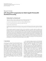
2.1. Observation model
In this section, we propose the problem and the model
of super-resolution reconstruction. Define that a low-
resolution image sequence is
{Y
k
}, N
1
× N
2
pixels, as our
measured data. An HR image X
, qN
1
× qN

2
pixels, is to be es-
timated from the LR sequences, where q is an integer-valued
interpolation factor in both the horizontal and vertical direc-
tions. To reduce the computational complexity, each frame
is separated into overlapping blocks (the shadow blocks as
shown in Figures 1(a) and 1(b)).
For convenience of notation, all overlapping blocked
frames will be presented as vector, ordered column-wise lex-
icographically. Namely, the overlapping blocked LR frame is
Y
k
∈ R
M
2
(M
2
× 1) and the overlapping blocked HR frame
is X
∈ R
q
2
M
2
(L
2
× 1orq
2
M
2

× 1). We assume that the two
images are related via the following equation:
Y
k
= D
k
H
k
F
k
X + V
k
, k = 1, 2, , N,(1)
where X
is blurred, decimated, down sampled, and contam-
inated by additive noise, giving Y
k
(t). The matrix F
k
(F ∈
R
q
2
M
2
×q
2
M
2
) stands for the geometric warp (translation) be-

tween the images X
and Y
k
. H
k
is the blur matrix which is a
space and time invariant and H
k
∈ R
q
2
M
2
×q
2
M
2
. D
k
is the dec-
imation matrix assumed constant and D
k
∈ R
M
2
×q
2
M
2
. V

k
is
a system noise and V
k
∈ R
M
2
.
Typically, many available estimators that estimate an HR
image from a set of noisy LR images are not exclusively based
on the LR measurement. They are also based on many as-
sumptions such as noise or motion models and these models
are not supposed to be exactly true, as they are merely math-
ematically convenient formulations of some general prior in-
formation. When the fundamental assumptions of data and
V. Patanavijit and S. Jitapunkul 5
qN
2
qN
1
X
X
(a) High-resolution image
N
2
N
1
Y
1
Y

2
···
Y
N
{Y
k
}
(b) Low-resolution image sequence
L
L
X
Degradation
process
M
Y
k
M
(c) The relation between overlapping blocked HR image and over-
lapping blocked LR image sequence
Figure 1: The observation model.
noise models do not faithfully describe the measured data,
the estimator performance degrades. Moreover, existence of
outliers defined as data points with different distributional
characteristics than the assumed model will produce erro-
neous estimates. Estimators promising optimality for a lim-
ited class of data and noise models may not be the most effec-
tive overall approach. Often, suboptimal estimation methods
that are not as sensitive to modeling and data errors may pro-
duce better and more stable results (robustness).
A popular family of estimators is the ML-type estimators

(M estimators) [50]. We rewrite the definition of these esti-
mators in the super-resolution reconstruction framework as
the following minimization problem:

X = ArgMin
X

N

k=1
ρ

D
k
H
k
F
k
X − Y
k


,(2)
where ρ(
·) is a robust error norm. To minimize (2), the in-
tensity at each pixel of the expected image must be close to
those of original image.
2.2. L1 norm estimator
A popular family of robust estimators is the L1 norm esti-
mators (ρ(x)

=x) that are used in super-resolution prob-
lem [52–55]. We rewrite the definition of these estimators in
the super-resolution context as the following minimization
problem:
X
= ArgMin
X

N

k=1


D
k
H
k
F
k
X − Y
k



. (3)
The L1 norm is not sensitive to outliers b ecause the in-
fluence function, ρ

(·), is constant and bounded but the L1
norm produces an estimator with higher variance than the

optimal L2 (quadratic) norm. The L1 norm function (ρ(
·))
and its influence function (ρ

(·)) are shown in Figures 2(a-1)
and 2(a-2), respectively.
2.3. L2 norm estimator
Another popular family of estimators is the L2 norm esti-
mators that are used in super-resolution problem [28, 29,
45–49]. We rewrite the definition of these estimators in
the super-resolution context as the following minimization
problem:
X
= ArgMin
X

N

k=1


D
k
H
k
F
k
X − Y
k



2
2

. (4)
The L2 norm produces estimator with lower variance
than the optimal L1 norm, but the L2 norm is very sensi-
tive to outliers because the influence function increases lin-
early and without bound. The L2 norm function (ρ(
·)) and
its influence function (ρ

(·)) are shown in Figures 2(b-1) and
2(b-2), respectively.
6 EURASIP Journal on Advances in Signal Processing
ρ
L1
(x)
x
(a-1)L1normfunction
ρ

L1
(x)
x
1
−1
(a-2) L1 norm influence function
ρ
L2

(x)
x
(b-1) L2 norm function
ρ

L2
(x)
x
(b-2) L2 norm influence function
ρ
LOR
(x)
x
−TT
(c-1) Lorentzian norm function
ρ

LOR
(x)
x
−T
T
(c-2) Lorentzian norm influence function
Figure 2: The norm function and the influence function.
2.4. Robust norm estimator
A robust estimation is an estimated technique that is resis-
tant to such outliers. In SRR framework, outliers are mea-
sured images or corrupted images that are highly inconsistent
with the high-resolution original image. Outliers may arise
from several reasons such as procedural measurement error,

noise and inaccurate mathematical model. Outliers should
be investigated carefully, therefore we need to analyze the
outlier in a way which minimizes their effect on the esti-
mated model. L2 norm estimation is highly susceptible to
even small numbers of discordant observations or outliers.
For L2 norm estimation, the influence of the outlier is much
larger than the other measured data because L2 norm esti-
mation weights the error quadraticly. Consequently, the ro-
bustness of L2 norm estimation is poor.
Much can be improved if the influence is bounded in one
way or another. This is exactly the general idea of applying
a robust error norm. Instead of using the sum of squared
differences (4), this error norm should be selected such that
above a given level of x its influence is ruled out. In addition,
one would like to have ρ(x) being smooth so that numerical
minimization of (5)isnottoodifficult. The suitable choice
(among others) is so-called Lorentzian error norm [65–68]
that is defined in (6). We rewrite the definition of these esti-
mators in the super-resolution context as the following min-
imization problem:
X
= ArgMin
X

N

k=1
ρ
LOR


D
k
H
k
F
k
X − Y
k


,(5)
ρ
LOR
(x) = log

1+
1
2

x
T

2

. (6)
The parameter T is Lorentzian constant parameter that
is a soft threshold value. For values of x smaller than T, the
function follows the L2 norm. For values larger than T, the
function gets saturated. Consequently, for small values of x,
the derivative of ρ


(x) = ∂{ρ(x)}/∂x of ρ(x)isnearlyacon-
stant. But for large values of x (for outliers), it becomes nearly
zero. Therefore, in a Gauss-Newton style of optimization, the
Jacobian matrix is virtually zero for outliers. Only residuals
that are about as large as T or smaller than that play a role.
From L1 and L2 norm estimation point of view,
Lorentzian’s norm is equivalent to the L1 norm for large
V. Patanavijit and S. Jitapunkul 7
value. But for normally distributed data, the L1 norm pro-
duces estimates with higher variance than the optimal L2
(quadratic) norm, so Lorentzian’s norm is designed to be
quadratic for small values. The Lorentzian norm function
(ρ(
·)) and its influence function (ρ

(·)) are shown in Figures
2(c-1) and 2(c-2), respectively.
3. ROBUST SUPER-RESOLUTION RECONSTRUCTION
This section proposes the robust SRR using L1, L2, and
Lorentzian norm minimization with different regularization
functions. Typically, super-resolution reconstruction is an
inverse problem [45–49] thus the process of computing an
inverse solution can be, and often is, extremely unstable in
that a small change in measurement (such as noise) can lead
to an enormous change in the estimated image (SR image).
Therefore, super-resolution reconstruction is an ill-posed or
ill-condition problem. An important point is that it is com-
monly possible to stabilize the inversion process by imposing
additional constraints that bias the solution, a process that is

generally referred to as regularization. Regularization is fre-
quently essential to produce a usable solution to an other-
wise intractable ill-posed or ill-conditioned inverse problem.
Hence, considering regularization in super-resolution algo-
rithm as a means for picking a stable solution is very useful,
if not necessary. Also, regularization can help the algorithm
to remove artifacts from the final answer and improve the
rate of convergence.
3.1. L1 norm SRR with Laplacian regularized
function [53]
A regularization term compensates the missing measurement
information with some general prior information about the
desirable HR solution, and is usually implemented as a
penalty factor in the generalized minimization cost function.
From (3), we rewrite the definition of these estimators in
the super-resolution context as the following minimization
problem:
X
= ArgMin
X

N

k=1


D
k
H
k

F
k
X − Y
k


+ λ · Υ(X)

. (7)
In general, Tikhonov regularization Υ(
·)wasreplacedby
matrix realization of the Laplacian kernel [53], the most clas-
sical and simplest regularization cost function, and where the
Laplacian kernel is defined as
Γ
=
1
8
⎡
⎢
⎣
111
1
−81
111
⎤
⎥
⎦
. (8)
Combining the Laplacian regularization, we propose the

solution of the super-resolution problem as follows:
X
= ArgMin
X

N

k=1


D
k
H
k
F
k
X − Y
k


+ λ · (ΓX)
2

. (9)
By the steepest descent method, the solution of problem
(9)isdefinedas

X
n+1
=


X
n
+ β ·

N

k=1
G
T
k
H
T
k
D
T
k
sign

D
k
H
k
G
k

X
n
− Y
k



−

λ ·

Γ
T
Γ


X
n


,
(10)
where β is a scalar defining the step size in the direction of
the gradient.
3.2. L1 norm SRR with BTV (Bitotal variance)
function [52–55]
A robust regularization function called bilateral-TV (BTV)
was introduced in [51, 53], therefore the BTV regularization
is defined as
Υ(X)
=
P

l=−P
P


m=0
α
|m|+|l|


X − S
l
x
S
m
y
X


, (11)
where matrices (operators) S
l
x
and S
m
y
shift X by l and m pix-
els in horizontal and vertical directions, respectively, present-
ing several scales of derivatives. The scalar weight α,0<α<
1, is applied to give a spatially decaying effect to the summa-
tion of the regularization terms [51, 53]. Combining the BTV
regularization, we rewrite the definition of these estimators
in the super-resolution context as the following minimiza-
tion problem:

X
= ArgMin
X

N

k=1



D · H · G(k) · X(t) − Y(k)


+ λ

P

l=−P
P

m=0
α
|m|+|l|


X − S
l
x
S
m

y
X



.
(12)
By the steepest descent method, the solution of problem
(13)isdefinedas

X
n+1
(t)
=

X
n
(t)+β ·

N

k=1
G
T
k
H
T
k
D
T

k
sign

D
k
H
k
G
k

X
n
− Y
k


−
λ

P

l=−P
P

m=0
α
|m|+|l|

I − S
l

x
S
m
y

·
sign


X − S
l
x
S
m
y

X


.
(13)
8 EURASIP Journal on Advances in Signal Processing
3.3. L2 norm SRR with Laplacian regularized
function [28, 29]
From (4), we rewrite the definition of these estimators in
the super-resolution context as the following minimization
problem:
X
= ArgMin
X


N

k=1


D
k
H
k
F
k
X − Y
k


2
2

. (14)
Combining the Laplacian regularization, we propose the
solution of the super-resolution problem as follows:
X
= ArgMin
X

N

k=1



D
k
H
k
F
k
X − Y
k


2
2
+ λ · Υ(X)

, (15)
X
= ArgMin
X

N

k=1


D
k
H
k
F

k
X − Y
k


2
2
+ λ · (ΓX)
2

. (16)
By the steepest descent method, the solution of problem
(16)isdefinedas

X
n+1
=

X
n
+ β ·

N

k=1
F
T
k
H
T

k
D
T
k

Y
k
− D
k
H
k
F
k

X
n

−

λ ·

Γ
T
Γ


X
n



.
(17)
3.4. L2 norm SRR with BTV (Bitotal variance)
function [52–55]
Combining the BTV regularization, we propose the solution
of the super-resolution problem as follows:
X
= ArgMin
X

N

k=1



D · H · G(k) · X(t) − Y(k)


2
2
+ λ

P

l=−P
P

m=0
α

|m|+|l|


X − S
l
x
S
m
y
X



.
(18)
By the steepest descent method, the solution of problem
(18)isdefinedas

X
n+1
(t) =

X
n
(t)+β ·

N

k=1
F

T
k
H
T
k
D
T
k

Y
k
− D
k
H
k
F
k

X
n


−
λ

P

l=−P
P


m=0
α
|m|+|l|

I − S
l
x
S
m
y

·
sign


X − S
l
x
S
m
y

X


.
(19)
3.5. Lorentzian norm SRR with Laplacian
regularized function [69]
In this sec tion, we propose the novel robust SRR using

Lorentzian error norm. From ( 5), we rewrite the definition
of these robust estimators in the super-resolution context as
the following minimization problem:
X
= ArgMin
X

N

k=1
ρ
LOR

D
k
H
k
F
k
X − Y
k


,
ρ
LOR
(x) = log

1+
1

2

x
T

2

.
(20)
Combining the Laplacian regularization, we propose the
solution of the super-resolution problem as follows:
X
= ArgMin
X

N

k=1
ρ
LOR

D
k
H
k
F
k
X − Y
k


+ λ · Υ(X)

,
(21)
X
= ArgMin
X

N

k=1
ρ
LOR

D
k
H
k
F
k
X − Y
k

+ λ · (ΓX)
2

.
(22)
By the steepest descent method, the solution of problem
(22)isdefinedas


X
n+1
=

X
n
+ β ·

N

k=1
F
T
k
H
T
k
D
T
k
· ρ

LOR

Y
k
− D
k
H

k
F
k

X
n

−

λ · (Γ
T
Γ


X
n


(23)
ρ

LOR
(x) =
2x
2T
2
+ x
2
. (24)
3.6. Lorentzian norm SRR with Lorentzian-Laplacian

regularized function [69]
Combining the Lorentzian-Laplacian regularization, we pro-
pose the solution of the super-resolution problem as follows:
X
= ArgMin
X

N

k=1
ρ
LOR

D
k
H
k
F
k
X − Y
k

+ λ · ψ
LOR
(ΓX)

,
(25)
ψ
LOR

(x) = log

1+
1
2

x
T
g

2

. (26)
By the steepest descent method, the solution of problem
(25)isdefinedas

X
n+1
=

X
n
+ β ·

N

k=1
F
T
k

H
T
k
D
T
k
· ρ

LOR

Y
k
− D
k
H
k
F
k

X
n

−

λ · Γ
T
· ψ

LOR


Γ

X
n


(27)
ψ

LOR
(x) =
2x
2T
2
g
+ x
2
. (28)
V. Patanavijit and S. Jitapunkul 9
(a-1, ,m-1) Original
HR image (Frame 40)
(a-2) Corrupted
LR image
(noiseless)
(PSNR
=
32.1687 dB)
(a-3) L1 SRR
image with Lap
reg. (PSNR

=
32.1687 dB)
(β
= 1, λ = 0)
(a-4) L1 SRR
image with BTV
reg. (PSNR
=
32.1687 dB)
(β
= 1, λ =
0, P = 1,
α
= 0.7)
(a-5) L2 SRR
image with Lap
reg. (PSNR
=
34.2 dB)
(β
= 1, λ = 0)
(a-6) L2 SRR
image with BTV
reg. (PSNR
=
34.2 dB)
(β
= 1, λ =
0, P = 1,
α

= 0.7)
(a-7) Lor. SRR
image with Lap
reg. (PSNR
=
35.2853 dB)
(β
= 0.25,
λ
= 0, T = 3)
(a-8) Lor. SRR
image with
Lor-Lap reg.
(PSNR
=
35.2853 dB)
(β
=0.25, λ=0,
T
= 1, T
g
= 1)
(b-2) Corrupted
LR image
(AWGN:SNR
=
25 dB) (PSNR =
30.1214 dB)
(b-3) L1 SRR
image with Lap

reg. (PSNR
=
30.3719 dB)
(β
= 0.5, λ = 1)
(b-4) L1 SRR
image with BTV
reg. (PSNR
=
30.3295 dB)
(β
= 0.5,
λ
= 0.4,
P
= 2, α = 0.7)
(b-5) L2 SRR
image with Lap
reg. (PSNR
=
32.3688 dB)
(β
= 0.5, λ = 1)
(b-6) L2 SRR
image with BTV
reg. (PSNR
=
32.1643 dB)
(β
= 0.5, λ =

0.4, P = 1,
α
= 0.7)
(b-7) Lor. SRR
image with Lap
reg. (PSNR
=
32.2341 dB)
(β
= 0.5, λ = 1,
T
= 9)
(b-8) Lor. SRR
image with
Lor Lap reg.
(PSNR
=
32.3591 dB)
(β
= 0.5,
λ
= 0.75,
T
= 9, T
g
= 3)
(c-2) Corrupted
LR image
(AWGN:SNR
=

22.5 dB) (PSNR =
29.0233 dB)
(c-3) L1 SRR
image with Lap
reg. (PSNR
=
29.6481 dB)
(β
= 0.5, λ = 1)
(c-4) L1 S RR
image with BTV
reg. (PSNR
=
29.5322 dB)
(β
= 0.5,
λ
= 0.4,
P
= 1, α = 0.7)
(c-5) L2 SRR
image with Lap
reg. (PSNR
=
31.6384 dB)
(β
= 1, λ = 1)
(c-6) L2 SRR
image with BTV
reg. (PSNR

=
31.5935 dB)
(β
= 0.5,
λ
= 0.4,
P
= 1, α = 0.7)
(c-7) Lor. SRR
image with Lap
reg. (PSNR
=
31.4751 dB)
(β
= 0.5,
λ
= 1, T = 9)
(c-8) Lor. SRR
image with
Lor Lap reg.
(PSNR
=
31.6169 dB)
(β
= 0.5, λ = 1,
T
= 9, T
g
= 3)
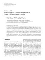
Figure 3: The experimental results of proposed method.

10 EURASIP Journal on Advances in Signal Processing
(d-2) Corrupted
LR image
(AWGN:SNR
=
20 dB) (PSNR =
27.5316 dB)
(d-3) L1 SRR
image with Lap
reg. (PSNR
=
28.7003 dB)
(β
= 0.5, λ = 1)
(d-4) L1 SRR
image with BTV
reg. (PSNR
=
28.9031 dB)
(β
= 0.5,
λ
= 0.4, P = 2,
α
= 0.7)
(d-5) L2 SRR
image with Lap
reg. (PSNR
=
30.6898 dB)

(β
= 0.5, λ = 1)
(d-6) L2 SRR
image with BTV
reg. (PSNR
=
31.0056 dB)
(β
= 0.5,
λ
= 0.3, P = 2,
α
= 0.7)
(d-7) Lor. SRR
image with Lap
reg. (PSNR
=
30.5472 dB)
(β
= 0.5,
λ
= 1, T = 9)
(d-8) Lor. SRR
image with
Lor Lap reg.
(PSNR
=
30.7486 dB)
(β
= 0.5, λ = 1,

T
= 9, T
g
= 5)
(e-2) Corrupted
LR image
(AWGN:SNR
=
17.5 dB) (PSNR =
25.7332 dB)
(e-3) L1 SRR
image with Lap
reg. (PSNR
=
27.5771 dB)
(β
= 1, λ = 1)
(e-4) L1 SRR
image with BTV
reg. (PSNR
=
27.7575 dB)
(β
= 0.5,
λ
= 0.5, P = 1,
α
= 0.7)
(e-5) L2 SRR
image with Lap

reg. (PSNR
=
29.3375 dB)
(β
= 0.5, λ = 1)
(e-6) L2 SRR
image with BTV
reg. (PSNR
=
29.4085 dB)
(β
= 0.5,
λ
= 0.5, P = 1,
α
= 0.7)
(e-7) Lor. SRR
image with Lap
reg. (PSNR
=
29.4712 dB)
(β
= 0.5, λ = 1,
T
= 5)
(e-8) Lor. SRR
image with
Lor Lap reg.
(PSNR
=

29.691 dB)
(β
= 0.5, λ = 1,
T
= 5, T
g
= 5)
(f-2) Corrupted
LR image
(AWGN:SNR
=
15 dB) (PSNR =
23.7086 dB)
(f-3) L1 S RR
image with Lap
reg. (PSNR
=
26.2641 dB)
(β
= 0.5, λ = 1)
(f-4) L1 SRR
image with BTV
reg. (PSNR
=
26.9064 dB)
(β
= 0.5,
λ
= 0.8, P = 1,
α

= 0.7)
(f-5) L2 SRR
image with Lap
reg. (PSNR
=
27.6671 dB)
(β
= 0.5, λ = 1)
(f-6) L2 S RR
image with BTV
reg. (PSNR
=
27.8418 dB)
(β
= 0.5,
λ
= 0.3, P = 2,
α
= 0.7)
(f-7) Lor. SRR
image with Lap
reg. (PSNR
=
28.1516 dB)
(β
= 0.5, λ = 1,
T
= 5)
(f-8) Lor. SRR
image with

Lor Lap reg.
(PSNR
=
28.4389 dB)
(β
= 0.5, λ = 1,
T
= 5, T
g
= 9)
Figure 3: continued.
V. Patanavijit and S. Jitapunkul 11
(g-2) Corrupted
LR image
(Poisson) (PSNR
= 27.9071 dB)
(g-3) L1 SRR
image with Lap
reg. (PSNR
=
28.9197 dB)
(β
= 1, λ = 1)
(g-4) L1 SRR
image with BTV
reg. (PSNR
=
29.1201 dB)
(β
= 0.5,

λ
= 0.4, P = 2,
α
= 0.7)
(g-5) L2 SRR
image with Lap
reg. (PSNR
=
30.7634 dB)
(β
= 0.5, λ = 1)
(g-6) L2 SRR
image with BTV
reg. (PSNR
=
30.8631 dB)
(β
= 0.5,
λ
= 0.5, P = 1,
α
= 0.7)
(g-7) Lor. SRR
image with Lap
reg. (PSNR
=
30.6934 dB)
(β
= 0.5, λ = 1,
T

= 9)
(g-8) Lor. SRR
image with
Lor Lap reg.
(PSNR
=
30.8829 dB)
(β
= 0.5, λ = 1,
T
= 5, T
g
= 9)
(h-2) Corrupted
LR image (S&P:D
= 0.005) (PSNR =
29.0649 dB)
(h-3) L1 SRR
image with Lap
reg. (PSNR
=
29.5041 dB)
(β
= 1, λ = 1)
(h-4) L1 SRR
image with BTV
reg. (PSNR
=
29.0649 dB)
(β

= 1,
λ
= 0.5, P = 2,
α
= 0.7)
(h-5) L2 SRR
image with Lap
reg. (PSNR
=
31.5021 dB)
(β
= 0.5, λ = 1)
(h-6) L2 SRR
image with BTV
reg. (PSNR
=
30.4617 dB)
(β
= 0.5,
λ
= 0.4, P = 1,
α
= 0.7)
(h-7) Lor. SRR
image with Lap
reg. (PSNR
=
34.7155 dB)
(β
= 1,

λ
= 0.25, T = 9)
(h-8) Lor. SRR
image with
Lor Lap reg.
(PSNR
=
34.7921 dB)
(β
= 1,
λ
= 0.25, T = 9,
T
g
= 3)
(i-2) (S&P:D =
0.01) Corrupted
LR image (PSNR
= 26.4446 dB)
(i-3) L1 SRR
image with Lap
reg. (PSNR
=
27.7593 dB)
(β
= 1, λ = 1)
(i-4) L1 SRR
image with BTV
reg. (PSNR
=

26.4446 dB)
(β
= 1,
λ
= 0.5, P = 1,
α
= 0.7)
(i-5) L2 SRR
image with Lap
reg. (PSNR
=
29.8395 dB)
(β
= 0.5, λ = 1)
(i-6) L2 SRR
image with BTV
reg. (PSNR
=
28.0337 dB)
(β
= 0.5,
λ
= 0.4, P = 1,
α
= 0.7)
(i-7) Lor. SRR
image with Lap
reg. (PSNR
=
34.7194 dB)

(β
= 1,
λ
= 0.25, T = 5)
(i-8) Lor. SRR
image with
Lor Lap reg.
(PSNR
=
34.7783 dB)
(β
= 1,
λ
= 0.25, T = 9,
T
g
= 3)
Figure 3: continued.
12 EURASIP Journal on Advances in Signal Processing
(j-2) Corrupted
LR image (S&P:D
= 0.015) (PSNR =
25.276 dB)
(j-3) L1 SRR
image with Lap
reg. (PSNR
=
26.9247 dB)
(β
= 1, λ = 1)

(j-4) L1 SRR
image with BTV
reg. (PSNR
=
25.276 dB)
(β
= 1,
λ
= 0.5, P = 1,
α
= 0.7)
(j-5) L2 SRR
image with Lap
reg. (PSNR
=
28.7614 dB)
(β
= 0.5, λ = 1)
(j-6) L2 SRR
image with BTV
reg. (PSNR
=
26.8671 dB)
(β
= 0.5,
λ
= 0.4, P = 1,
α
= 0.7)
(j-7) Lor. SRR

image with Lap
reg. (PSNR
=
34.6991 dB)
(β
= 1,
λ
= 0.25, T = 5)
(j-8) Lor. SRR
image with
Lor Lap reg.
(PSNR
=
34.7001 dB)
(β
= 1,
λ
= 0.25, T = 9,
T
g
= 3)
(k-2) (Speckle:
V
= 0.01)
Corrupted LR
image (PSNR
=
27.6166 dB)
(k-3) L1 SRR
image with Lap

reg. (PSNR
=
28.8289 dB)
(β
= 0.5, λ = 1)
(k-4) L1 SRR
image with BTV
reg. (PSNR
=
28.8656 dB)
(β
= 0.5,
λ
= 0.7, P = 1,
α
= 0.7)
(k-5) L2 SRR
image with Lap
reg. (PSNR
=
30.6139 dB)
(β
= 0.5, λ = 1)
(k-6) L2 SRR
image with BTV
reg. (PSNR
=
30.613 dB)
(β
= 0.5,

λ
= 0.5, P = 1,
α
= 0.7)
(k-7) Lor. SRR
image with Lap
reg. (PSNR
=
29.8499 dB)
(β
= 0.5, λ = 1,
T
= 9)
(k-8) Lor. SRR
image with
Lor Lap reg.
(PSNR
=
30.1287 dB)
(β
= 0.5, λ = 1,
T
= 9, T
g
= 5)
(l-2) (Speckle:
V
= 0.02)
Corrupted LR
image (PSNR

=
25.3563 dB)
(l-3) L1 SRR
image with Lap
reg. (PSNR
=
27.5527 dB)
(β
= 0.5, λ = 1)
(l-4) L1 S RR
image with BTV
reg. (PSNR
=
27.8283 dB)
(β
= 0.5,
λ
= 0.6, P = 1,
α
= 0.7)
(l-5) L2 SRR
image with Lap
reg. (PSNR
=
28.9409 dB)
(β
= 0.5, λ = 1)
(l-6) L2 SRR
image with BTV
reg. (PSNR

=
28.8859 dB)
(β
= 0.5,
λ
= 0.5, P = 1,
α
= 0.7)
(l-7) Lor. SRR
image with Lap
reg. (PSNR
=
28.5018 dB)
(β
= 0.5, λ = 1,
T
= 1)
(l-8) Lor. SRR
image with
Lor Lap reg.
(PSNR
=
28.9779 dB)
(β
= 0.5, λ = 1,
T
= 1, T
g
= 3)
Figure 3: continued.

V. Patanavijit and S. Jitapunkul 13
(m-2) (Speckle:
V
= 0.03)
Corrupted LR
image (PSNR
=
24.0403 dB)
(m-3) L1 SRR
image with Lap
reg. (PSNR
=
26.8165 dB)
(β
= 0.5, λ = 1)
(m-4) L1 SRR
image with BTV
reg. (PSNR
=
27.2429 dB) (β =
0.5, λ = 0.5, P =
1, α = 0.7)
(m-5) L2 SRR
image with Lap
reg. (PSNR
=
27.7654 dB)
(β
= 0.5, λ = 1)
(m-6) L2 SRR

image with BTV
reg. (PSNR
=
27.3751 dB)
(β
= 0.5,
λ
= 0.4, P = 1,
α
= 0.7)
(m-7) Lor. SRR
image with Lap
reg. (PSNR
=
27.9468 dB)
(β
= 0.5, λ = 1,
T
= 1)
(m-8) Lor. SRR
image with
Lor Lap reg.
(PSNR
=
28.4418 dB)
(β
= 0.5, λ = 1,
T
= 1, T
g

= 3)
Figure 3: continued.
4. EXPERIMENTAL RESULT
This section presents the experiments and results obtained
by the proposed robust SRR methods using Lorentzian
norm w ith Laplacian and Lorentzian-Laplacian regulariza-
tions that are calculated by (23)and(27). To demonstrate the
proposed robust SRR performance, the results of L1 norm
SRR with Laplacian and BTV regularizations calculated by
(10)and(13) and the results of L2 norm SRR with Lapla-
cian and BTV regularizations calculated by (17)and(19)are
presented in order to compare the performance.
These experiments are implemented in MATLAB and the
blocksizeisfixedat8× 8(16× 16 for overlapping block).
In this experiment, we create a sequence of LR frames by
using the 40th frame Susie sequence that is QCIF format
(176
× 144) and using the Lena (standard image). First, we
shifted this HR image by a pixel in the vertical direction.
Then, to simulate the effect of camera PSF, this shifted im-
age was convolved with a symmetric Gaussian low-pass fil-
ter of size 3
× 3 with standard deviation equal to one. The
resulting image was subsampled by the factor of 2 in each
direction. The same approach with different motion vectors
(shifts) in vertical and horizontal directions was used to pro-
duce 4 LR images from the original scene. We added different
noise model to the resulting LR fr ames. Next, we use 4 LR
frames to generate the high-resolution image by the different
SRR methods. (The criterion for parameter selection in this

paper was to choose parameters which produce both most
visually appealing results and highest PSNR. Therefore, to
ensure fairness, each experiment was repeated several times
with different parameters and the best result of each experi-
ment was chosen [52–55].)
4.1. Susie sequence (the 40th Frame)
Noiseless
The original HR image is shown in Figure 3(a-1) and one
of the corrupted LR images is shown in Figure 3(a-2). Next,
the results of implementing the super-resolution method us-
ing L1 estimator with Laplacian regularization, L1 estimator
with BTV regularization, L2 estimator with Laplacian regu-
larization, L2 estimator with BTV regularization, Lorentzian
estimator with Laplacian regularization and Lorentzian es-
timator with Lorentzian-Laplacian regularization are shown
in Figures 3(a-3)–3(a-8), respectively. Due to noiseless ef-
fect, the results of SRR without regularization give a better
result than the SRR with regularization. From the results,
Lorentzian estimator can efficiently reconstruct the noiseless
image than L1 and L2 estimator, about 1–3 dB, respectively.
Additive white Gaussian noise
This experiment is 5 AWGN cases at SNR
= 25, 22.5, 20,
17.5, and 15 dB, respectively, and the or iginal HR images are
shown in Figures 3(b-1)–3(f-1), respectively. The corrupted
images at SNR
= 25, 22.5, 20, 17.5, and 15 dB are show in
Figures 3(b-2)–3(f-2), respectively.
At the high SNR (SNR
= 25 and 22.5 dB) or low-noise

power, the L2 estimator results (with Laplacian and BTV reg-
ularizations) give slightly higher PSNR than Lorentzian esti-
mator result (with Laplacian and Lorentzian-Laplacian reg-
ularizations). However, L2 and Lorentzian estimator result
have higher PSNR than L1 estimator results. At SNR
= 25 dB
and SNR
= 22.5 dB, the result of L1 estimator with Laplacian
regularization, L1 estimator with BTV regularization, L2 esti-
mator with Laplacian regularization, L2 estimator with BTV
regularization, Lorentzian estimator with Laplacian regular-
ization, and Lorentzian estimator with Lorentzian-Laplacian
regularization estimation are shown in Figures 3(b-3)–3(b-
8) and 3(c-3)–3(c-8), respectively.
At low SNR (SNR
= 20 dB, SNR = 17.5 dB, and SNR
= 15 dB) or high-noise power, the Lorentzian estimator re-
sults (with Lorentzian-Laplacian regularization and Lapla-
cian regularization) give the best performance than L2 esti-
mator result (with Laplacian and BTV regularization) and L1
estimator results (with Laplacian and BTV regularization).
At SNR
= 20 dB, SNR = 17.5 dB, and SNR = 15 dB, the results
14 EURASIP Journal on Advances in Signal Processing
of L1 estimator with Laplacian regularization, L1 estimator
with BTV regularization, L2 estimator with Laplacian regu-
larization, L2 estimator with BTV regularization, Lorentzian
estimator with Laplacian regularization and Lorentzian es-
timator with Lorentzian-Laplacian regularization estimation
are shown in Figures 3(d-3)–3(d-8), 3(e-3)–3(e-8), and 3(f-

3)–3(f-8), respectively.
From the results, the L2 estimator gives the best result
for SRR estimation than Lorentzian or L1 estimator a t low-
noise power because the AWGN distributional characteristic
is a quadratic model that is similar to L2 model. However, at
high-noise power, the Lorentzian estimator will give the bet-
ter result than L2 estimator since the L2 norm is very sensi-
tive to outliers where the influence function increases linearly
and without bound.
Poisson noise
The original HR image is shown in Figure 3(g-1) and one
of corrupted LR images is shown in Figure 3(g-2). The
Lorentzian estimator results with Lorentzian-Laplacian reg-
ularization give the highest PSNR than the Lorentzian es-
timator results with Laplacian regularization, L2 estimator
result with Laplacian and BTV regularizations, and L1 esti-
mator result with Laplacian and BTV regularization. The re-
sult of implementing the super-resolution method using L1
estimator with Laplacian regularization, L1 estimator with
BTV regularization, L2 estimator with Laplacian regulariza-
tion, L2 estimator with BTV regularization, Lorentzian esti-
mator with Laplacian regularization and Lorentzian estima-
tor with Lorentzian-Laplacian Regularization are shown in
Figures 3(g-3)–3(g-8), respectively.
From the results, the Lorentzian estimator will give the
best result than L1 and L2 estimators since the power of noise
is slightly high and the distribution of noise is not quadratic
model (the L2 estimator cannot estimate the no quadratic
model effectively).
Salt and pepper noise

This is 3 salt and pepper noise cases at D
= 0.005, D = 0.01,
and D
= 0.015, respectively, a nd the original HR images
are shown in Figures 3(h-1)–3(j-1), respectively. The cor-
rupted images at D
= 0.005, D = 0.01, and D = 0.015 are
shown in Figures 3(h-2), 3(i-2), and 3(j-2), respectively. The
Lorentzian estimator results (with Laplacian and Lorentzian-
Laplacian regularizations results) give dramatically higher
PSNR than L1 estimator results (with Laplacian and BTV
regularization results) and L2 estimator result (with Lapla-
cian and BTV regularizations results).
At D
= 0.005, D = 0.01, and D = 0.015, the results
of L1 estimator with Laplacian regularization, L1 estimator
with BTV regularization, L2 estimator with Laplacian regu-
larization, L2 estimator with BTV regularization, Lorentzian
estimator with Laplacian regularization, and Lorentzian es-
timator with Lorentzian-Laplacian regularization estimation
are shown in Figures 3(h-3)–3(h-8), 3(i-3)–3(i-8), and 3(j-
4)–3(j-8), respectively.
From the results, the Lorentzian estimator with Laplacian
regularization and the Lorentzian estimator with Lorentzian-
Laplacian regularization can outstandingly efficiently recon-
struct the image that is corrupted by salt and pepper noise
than L1 and L2 estimator about 4-5 dB. The Lorentzian esti-
mator gives the best result for SRR estimation than L1 or L2
estimator because the Lorentzian estimator is designed to b e
robustness and reject outliers, the norm must be more for-

giving about outliers; that is, it should increase less rapidly
than L2.
Speckle noise
The last experiment is 3 speckle noise cases for 40th frame
Susie sequence at V
= 0.01, V = 0.02, and V = 0.03, respec-
tively, and the original HR images are shown in Figures 3(k-
1)–3(m-1), respectively. The corrupted images at V
= 0.01,
V
= 0.02, and V = 0.03areshoweninFigures3(k-2), 3(l-2)
and 3(m-2), respectively.
At low-noise power (V
= 0.01), the L2 estimator re-
sults (with Laplacian and BTV regularizations) give slightly
higher PSNR than Lorentzian estimator results (with Lapla-
cian and Lorentzian-Laplacian regularizations). However, L2
and Lorentzian estimators results have higher PSNR than
L1 estimator results (with Laplacian and BTV regulariza-
tions). The results of implementing the super-resolution
method using L1 estimator with Laplacian regularization,
L1 estimator with BTV regularization, L2 estimator with
Laplacian regularization, L2 estimator with BTV regulariza-
tion, Lorentzian estimator with Laplacian regularization and
Lorentzian estimator with Lorentzian-Laplacian regulariza-
tion are show n in Figures 3(k-3) and 3(k-8), respectively.
At high-noise power (V
= 0.02 and V = 0.03), the
Lorentzian estimator results (with Laplacian and Lorentzian-
Laplacian regularizations) give the best performance than L2

estimator results (with Laplacian and BTV regularizations)
and L1 estimator results (with Laplacian and BTV regular-
izations). At V
= 0.02 dB and V = 0.03, the results of L1
estimator with Laplacian regularization, L1 estimator with
BTV regularization, L2 estimator with Laplacian regulariza-
tion, L2 estimator with BTV regularization, Lorentzian es-
timator with Laplacian regularization, and Lorentzian esti-
mator with Lorentzian-Laplacian regularization are shown in
Figures 3(l-3)–3(l-8) and 3(m-3)–3(m-8), respectively.
From the results, the Lorentzian estimator can efficiently
reconstruct the image that is corrupted by speckle noise
at hig h-noise power than L1 and L2 estimators because
Lorentzian estimator is more robust for estimation to the
high-power outlier than L1 and L2 estimators.
4.2. Lena (the standard image)
Noiseless
The original HR image is shown in Figure 4(a-1) and one
of the corrupted LR images is shown in Figure 4(a-2). Next,
the results of implementing the super-resolution method us-
ing L1 estimator with Laplacian regularization, L1 estima-
tor with BTV regularization, L2 estimator with Laplacian
V. Patanavijit and S. Jitapunkul 15
(a-1, ,k-1)
Original HR image
(a-2) Corrupted
LR image
(noiseless)
(PSNR
=

28.8634 dB)
(a-3) L1 SRR
image with Lap
reg. (PSNR
=
28.8634 dB)
(β
= 1, λ = 0)
(a-4) L1 SRR
image with BTV
reg. (PSNR
=
28.8634 dB)
(β
= 1, λ = 0,
P
= 1, α = 0.7)
(a-5) L2 SRR
image with Lap
reg. (PSNR
=
30.8553 dB)
(β
= 1, λ = 0)
(a-6) L2 SRR
image with BTV
reg. (PSNR
=
30.8553 dB)
(β

= 1, λ = 0,
P
= 1, α = 0.7)
(a-7) Lor. SRR
image with Lap
reg. (PSNR
=
31.9565 dB)
(β
= 0.25, λ = 0,
T
= 3)
(a-8) Lor. SRR
image with
Lor-Lap reg.
(PSNR
=
31.9565 dB)
(β
= 0.25, λ = 0,
T
= 3, T
g
= 1)
(b-2) Corrupted
LR image
(AWGN:SNR
=
25 dB) (PSNR =
27.8884 dB)

(b-3) L1 SRR
image with Lap
reg. (PSNR
=
27.949 dB)
(β
= 0.5, λ = 1)
(b-4) L1 SRR
image with BTV
reg. (PSNR
=
27.8884 dB)
(β
= 0.5,
λ
= 0.25, P = 1,
α
= 0.7)
(b-5) L2 SRR
image with Lap
reg. (PSNR
=
29.6579 dB)
(β
= 0.5, λ = 0.5)
(b-6) L2 SRR
image with BTV
reg. (PSNR
=
29.58 dB) (β =

0.5, λ = 0.25,
P
= 1, α = 0.7)
(b-7) Lor. SRR
image with Lap
reg. (PSNR
=
29.7359 dB)
(β
= 1, λ = 0.5,
T
= 15)
(b-8) Lor. SRR
image with
Lor Lap reg.
(PSNR
=
29.7712 dB)
(β
= 0.5, λ = 0.5,
T
= 19, T
g
= 5)
(c-2) Corrupted
LR image
(AWGN:SNR
=
22.5 dB) (PSNR =
27.2417 dB)

(c-3) L1 S RR
image with Lap
reg. (PSNR
=
27.4918 dB)
(β
= 0.5, λ = 1)
(c-4) L1 SRR
image with BTV
reg. (PSNR
=
27.3968 dB)
(β
= 0.5,
λ
= 0.75, P = 1,
α
= 0.7)
(c-5) L2 S RR
image with Lap
reg. (PSNR
=
29.1611 dB)
(β
= 0.5, λ = 1)
(c-6) L2 S RR
image with BTV
reg. (PSNR
=
29.0775 dB)

(β
= 0.5,
λ
= 0.25,
P
= 1, α = 0.7)
(c-7) Lor. SRR
image with Lap
reg. (PSNR
=
29.1927 dB)
(β
= 0.5, λ = 1,
T
= 19)
(c-8) Lor. SRR
image with
Lor Lap reg.
(PSNR
=
29.2183 dB)
(β
=0.5, λ=0.75,
T
= 19, T
g
= 9)
Figure 4: The experimental results of proposed method.
16 EURASIP Journal on Advances in Signal Processing
(d-2) Corrupted

LR image
(AWGN:SNR
=
20 dB) (PSNR =
26.2188 dB)
(d-3) L1 SRR
image with Lap
reg. (PSNR
=
26.7854 dB)
(β
= 0.5, λ = 1.0)
(d-4) L1 SRR
image with BTV
reg. (PSNR
=
26.7197 dB)
(β
= 0.5,
λ
= 0.8, P = 1,
α
= 0.7)
(d-5) L2 SRR
image with Lap
reg. (PSNR
=
28.6024 dB)
(β
= 0.5, λ = 1)

(d-6) L2 SRR
image with BTV
reg. (PSNR
=
28.5195 dB)
(β
= 0.5,
λ
= 0.5, P = 1,
α
= 0.7)
(d-7) Lor. SRR
image with Lap
reg. (PSNR
=
28.561 dB)
(β
= 0.5, λ = 1,
T
= 19)
(d-8) Lor. SRR
image with
Lor Lap reg.
(PSNR
=
28.6383 dB)
(β
= 0.5, λ = 1,
T
= 19, T

g
= 5)
(e-2) Corrupted
LR image
(AWGN:SNR
=
17.5 dB) (PSNR =
24.9598 dB)
(e-3) L1 SRR
image with Lap
reg. (PSNR
=
26.0348 dB)
(β
= 0.5, λ = 1)
(e-4) L1 SRR
image with BTV
reg. (PSNR
=
26.0066 dB)
(β
= 0.5,
λ
= 0.75,
P
= 1, α = 0.7)
(e-5) L2 SRR
image with Lap
reg. (PSNR
=

27.8153 dB)
(β
= 0.5, λ = 1)
(e-6) L2 SRR
image with BTV
reg. (PSNR
=
27.964 dB)
(β
= 0.5,
λ
= 0.75,
P
= 1, α = 0.7)
(e-7) Lor. SRR
image with Lap
reg. (PSNR
=
27.7621 dB)
(β
= 0.5, λ = 1,
T
= 15)
(e-8) Lor. SRR
image with
Lor Lap reg.
(PSNR
=
27.9152 dB)
(β

= 0.5, λ = 1,
T
= 15, T
g
= 15)
(f-2) Corrupted
LR image
(AWGN:SNR
=
15 dB) (PSNR =
23.3549 dB)
(f-3) L1 SRR
image with Lap
reg. (PSNR
=
25.1488 dB)
(β
= 0.5, λ = 1)
(f-4) L1 S RR
image with BTV
reg. (PSNR
=
25.2642 dB)
(β
= 0.5,
λ
= 0.8,
P
= 1, α = 0.7)
(f-5) L2 SRR

image with Lap
reg. (PSNR
=
26.6406 dB)
(β
= 0.5, λ = 1)
(f-6) L2 SRR
image with BTV
reg. (PSNR
=
26.7713 dB)
(β
= 0.5, λ = 0.7,
P
= 1, α = 0.7)
(f-7) Lor. SRR
image with Lap
reg. (PSNR
=
26.7566 dB)
(β
= 0.5, λ = 1,
T
= 9)
(f-8) Lor. SRR
image with
Lor Lap reg.
(PSNR
=
26.7947 dB)

(β
= 0.5, λ = 1,
T
= 5, T
g
= 9)
Figure 4: continued.
V. Patanavijit and S. Jitapunkul 17
(g-2) Corrupted
LR image
(Poisson) (PSNR
= 26.5116 dB)
(g-3) L1 SRR
image with Lap
reg. (PSNR
=
26.9604 dB)
(β
= 0.5, λ = 1)
(g-4) L1 SRR
image with BTV
reg. (PSNR
=
26.8759 dB)
(β
= 0.5, λ = 0.8,
P
= 1, α = 0.7)
(g-5) L2 SRR
image with Lap

reg. (PSNR
=
28.719 dB)
(β
= 0.5, λ = 1)
(g-6) L2 SRR
image with BTV
reg. (PSNR
=
28.6848 dB)
(β
= 0.5, λ = 0.5,
P
= 1, α = 0.7)
(g-7) Lor. SRR
image with Lap
reg. (PSNR
=
28.6735 dB)
(β
= 0.5, λ = 1,
T
= 19)
(g-8) Lor. SRR
image with
Lor Lap reg.
(PSNR
=
28.7471 dB)
(β

= 0.5, λ = 1,
T
= 19, T
g
= 5)
(h-2) Corrupted
LR image (S&P:
D
= 0.005)
(PSNR
=
26.8577 dB)
(h-3) L1 SRR
image with Lap
reg. (PSNR
=
27.1149 dB)
(β
= 0.5, λ = 1)
(h-4) L1 SRR
image with BTV
reg. (PSNR
=
26.8577 dB)
(β
= 1, λ = 0.5,
P
= 1, α = 0.7)
(h-5) L2 SRR
image with Lap

reg. (PSNR
=
28.8495 dB)
(β
= 0.5, λ = 1)
(h-6) L2 SRR
image with BTV
reg. (PSNR
=
28.1438 dB)
(β
= 0.5, λ = 0.6,
P
= 1, α = 0.7)
(h-7) Lor. SRR
image with Lap
reg. (PSNR
=
31.1843 dB)
(β
= 1, λ = 0.25,
T
= 9)
(h-8) Lor. SRR
image with
Lor Lap reg.
(PSNR
=
31.2123 dB)
(β

= 1, λ = 0.5,
T
= 9, T
g
= 1)
(i-2) (S&P:
D
= 0.010)
Corrupted LR
image (PSNR
=
25.2677 dB)
(i-3) L1 SRR
image with Lap
reg. (PSNR
=
26.0569 dB)
(β
= 1, λ = 1)
(i-4) L1 SRR
image with BTV
reg. (PSNR
=
25.2677 dB)
(β
= 1, λ = 0.4,
P
= 1, α = 0.7)
(i-5) L2 SRR
image with Lap

reg. (PSNR
=
28.0346 dB)
(β
= 0.5, λ = 1)
(i-6) L2 SRR
image with BTV
reg. (PSNR
=
26.7979 dB)
(β
= 0.5, λ = 0.4,
P
= 1, α = 0.7)
(i-7) Lor. SRR
image with Lap
reg. (PSNR
=
31.0524 dB)
(β
= 1, λ = 0.25,
T
= 19)
(i-8) Lor. SRR
image with
Lor Lap reg.
(PSNR
=
31.0748 dB)
(β

= 1, λ = 0.25,
T
= 9, T
g
= 5)
Figure 4: continued.
18 EURASIP Journal on Advances in Signal Processing
(j-2) Corrupted
LR image (S&P:
D
= 0.015)
(PSNR
=
24.2190 dB)
(j-3) L1 SRR
image with Lap
reg. (PSNR
=
25.3534 dB)
(β
= 1, λ = 1)
(j-4) L1 SRR
image with BTV
reg. (PSNR
=
24.2202 dB)
(β
= 0.5, λ = 0.3,
P
= 1, α = 0.7)

(j-5) L2 SRR
image with Lap
reg. (PSNR
=
27.3188 dB)
(β
= 0.5, λ = 1)
(j-6) L2 SRR
image with BTV
reg. (PSNR
=
25.8242 dB)
(β
= 0.5, λ = 0.4,
P
= 1, α = 0.7)
(j-7) Lor. SRR
image with Lap
reg. (PSNR
=
30.0229 dB)
(β
= 1, λ = 0.25,
T
= 19)
(j-8) Lor. SRR
image with
Lor Lap reg.
(PSNR
=

31.0627 dB)
(β
= 1, λ = 0.25,
T
= 9, T
g
= 5)
(k-2) (Speckle)
Corrupted LR
image (PSNR
=
21.7994 dB)
(k-3) L1 SRR
image with Lap
reg. (PSNR
=
24.4215 dB)
(β
= 0.5, λ = 1)
(k-4) L1 SRR
image with BTV
reg. (PSNR
=
24.5102 dB)
(β
= 0.5, λ = 0.5,
P
= 1, α = 0.7)
(k-5) L2 SRR
image with Lap

reg. (PSNR
=
25.3165 dB)
(β
= 0.5, λ = 1)
(k-6) L2 SRR
image with BTV
reg. (PSNR
=
23.958 dB)
(β
= 0.5, λ = 0.4,
P
= 1, α = 0.7)
(k-7) Lor. SRR
image with Lap
reg. (PSNR
=
25.3136 dB)
(β
= 0.5, λ = 1,
T
= 1)
(k-8) Lor. SRR
image with
Lor Lap reg.
(PSNR
=
25.609 dB)
(β

= 0.5, λ = 1,
T
= 1, T
g
= 5)
Figure 4: continued.
regularization, L2 estimator with BTV regularization,
Lorentzian estimator with Laplacian regular ization and
Lorentzian estimator with Lorentzian-Laplacian regulariza-
tion are show n in Figures 4(a-3)–4(a-8), respectively.
Additive white Gaussian noise
This experiment is 5 AWGN cases at SNR
= 25, 22.5, 20,
17.5, and 15 dB, respectively, and the or iginal HR images are
shown in Figures 4(b-1)–4(f-1), respectively. The corrupted
images at SNR
= 25, 22.5, 20, 17.5, and 15 dB are shown in
Figures 4(b-2)–4(f-2), respectively.
At SNR
= 25, 22.5, 20, 17.5, and 15 dB, respectively,
the results of L1 estimator with Laplacian regularization,
L1 estimator with BTV regularization, L2 estimator with
Laplacian regularization, L2 estimator with BTV regulariza-
tion, Lorentzian estimator with Laplacian regularization and
Lorentzian estimator with Lorentzian-Laplacian regulariza-
tion estimation are shown in Figures 4(b-3)–4(b-8), 4(c-3)–
4(c-8), 4(d-3)–4(d-8), 4(e-3)–4(e-8), and 4(f-3)–4(f-8), re-
spectively. The Lorentzian estimator result (with Lorentzian-
Laplacian and Laplacian regularization) gives the best per-
formance than L2 estimator result (with Laplacian and BTV

regularization) and L1 estimator result (with Laplacian and
BTV regularizations).
Poisson noise
The original HR image is shown in Figure 4(g-1) and one
of corrupted LR images is shown in Figure 4(g-2). The
Lorentzian estimator result with Lorentzian-Laplacian reg-
ularization gives the highest PSNR than the Lorentzian esti-
mator result with Laplacian regularization, L2 estimator re-
sult with Laplacian and BTV regularization and L1 estima-
tor result with Laplacian and BTV regularization. The result
of implementing the super-resolution method using L1 esti-
mator with Laplacian regularization, L1 estimator with BTV
regularization, L2 estimator with Laplacian regularization,
L2 estimator with BTV regularization, Lorentzian estima-
tor with Laplacian regularization and Lorentzian estimator
with Lorentzian-Laplacian regularization are shown in Fig-
ures 4(g-3)–4(g-8), respectively.
V. Patanavijit and S. Jitapunkul 19
Salt and pepper noise
This experiment is 3 salt and pepper noise cases at D
= 0.005,
D
= 0.01 and D = 0.015, respectively, and the original HR
images are shown in Figures 4(h-1)–4(j-1) respectively. The
corrupted images at D
= 0.005, D = 0.010 and D = 0.015
are shown in Figures 4(h-2), 4(i-2), and 4(j-2), respectively.
The Lorentzian estimator results (with Lorentzian-Laplacian
and Laplacian regularization) give dramatically higher PSNR
than L1 estimator result (with Laplacian and BTV regular-

ization results) and L2 estimator results (with Laplacian and
BTV regularizations results).
At D
= 0.005, D = 0.01, and D = 0.015, the results
of L1 estimator with Laplacian regularization, L1 estimator
with BTV regularization, L2 estimator with Laplacian regu-
larization, L2 estimator with BTV regularization, Lorentzian
estimator with Laplacian regularization and Lorentzian es-
timator with Lorentzian-Laplacian regularization estimation
are shown in Figures 4(h-3)–4(h-8), 4(i-3)–4(i-8), and 4(j-
4)–4(j-8), respectively.
Speckle noise
The last experiment is speckle noise cases and the origi-
nalHRimagesareshowninFigure 4(k-1). The corrupted
image is shown in Figure 4(k-2). The Lorentzian estimator
result (with Lorentzian-Laplacian and Laplacian regulariza-
tion) gives the best performance than L2 estimator result
(with Laplacian and BTV regularizations) and L1 estimator
result (with Laplacian and BTV regularization). The result
of L1 estimator with Laplacian regularization, L1 estimator
with BTV regularization, L2 estimator with Laplacian regu-
larization, L2 estimator with BTV regularization, Lorentzian
estimator with Laplacian regularization and Lorentzian es-
timator with Lorentzian-Laplacian regularization are shown
in Figures 4(k-3)–4(k-8).
5. CONCLUSION
In this paper, we propose an alternate approach using a novel
robust estimation norm function (Lorentzian norm func-
tion) for SRR framework with Tikhonov and Lorentzian-
Tikhonov regularizations and the proposed robust SRR can

be effectively applied on the images that is corrupted by var-
ious noise models. Experimental results conducted clearly
that the proposed robust algorithm can well apply on the sev-
eral noise models such as noiseless, AWGN, Poisson noise,
and salt and pepper noise, and speckle noise and the pro-
posed a lgorithm can obviously improve the result in using
both subjective and objective measurements.
ACKNOWLEDGMENTS
The authors would like to express the grateful thanks to grant
from government research and development in cooperative
project between Department of Electrical Engineering and
Private Sector Research for supporting this work and devel-
opment under Chulalongkorn University.
REFERENCES
[1] C. A. Segall, R. Molina, and A. K. Katsaggelos, “High-
resolution images from low-resolution compressed video,”
IEEE Signal Processing Magazine, vol. 20, no. 3, pp. 37–48,
2003.
[2] D. Kundur and D. Hatzinakos, “Blind image deconvolution,”
IEEE Signal Processing Magazine, vol. 13, no. 3, pp. 43–64,
1996.
[3] D. Rajan, S. Chaudhuri, and M. V. Joshi, “Multi-objective su-
per resolution: concepts and examples,” IEEE Signal Processing
Magazine, vol. 20, no. 3, pp. 49–61, 2003.
[4] G. Demoment, “Image reconstruction and restoration:
overview of common estimation structures and problems,”
IEEE Transactions on Acoustics, Speech, and Signal Processing,
vol. 37, no. 12, pp. 2024–2036, 1989.
[5] M. K. Ng and N. K. Bose, “Mathematical analysis of super-
resolution methodology,” IEEE Signal Processing Magazine,

vol. 20, no. 3, pp. 62–74, 2003.
[6] M. G. Kang and S. Chaudhuri, “Super-resolution image recon-
struction,” IEEE Signal Processing Magazine,vol.20,no.3,pp.
19–20, 2003.
[7] S. Chaudhuri and D. R. Taur, “High-resolution slow-motion
sequencing,” IEEE Signal Processing Magazine, vol. 22, no. 2,
pp. 16–24, 2005.
[8] S. C. Park, M. K. Park, and M. G. Kang, “Super-resolution im-
age reconstruction: a technical overview,” IEEE Signal Process-
ing Magazine, vol. 20, no. 3, pp. 21–36, 2003.
[9] M. R. Banham and A. K. Katsaggelos, “Digital image restora-
tion,” IEEE Signal Processing Magazine, vol. 14, no. 2, pp. 24–
41, 1997.
[10] T. S. Huang and R. Y. Tsan, “Multiple frame image restora-
tion and registration,” in Advances in Computer Vision and Im-
age Processing, T. S. Huang, Ed., vol. 1, pp. 317–339, JAI Press,
Greenwich, Conn, USA, 1984.
[11] S. P. Kim, N. K. Bose, and H. M. Valenzuela, “Recursive recon-
struction of high resolution image from noisy undersampled
multiframes,” IEEE Transactions on Acoustics, Speech, and Sig-
nal Processing, vol. 38, no. 6, pp. 1013–1027, 1990.
[12] S. P. Kim and W Y. Su, “Recursive high-resolution reconstruc-
tion of blurred multiframe images,” IEEE Transactions on Im-
age Processing, vol. 2, no. 4, pp. 534–539, 1993.
[13] M. K. Ng and N. K. Bose, “Analysis of displacement errors
in high-resolution image reconstruction with multisensors,”
IEEE Transactions on Circuits and Systems I: Fundamental The-
ory and Applications, vol. 49, no. 6, pp. 806–813, 2002.
[14]N.K.Bose,M.K.Ng,andA.C.Yau,“Afastalgo-
rithm for image super-resolution from blurred observations,”

EURASIP Journal on Applied Signal Processing, vol. 2006, Arti-
cle ID 35726, 14 pages, 2006.
[15] A. J. Patti and Y. Altunbasak, “Artifact reduction for set theo-
retic super resolution image reconstruction with edge adaptive
constraints and higher-order inter polants,” IEEE Transactions
on Image Processing, vol. 10, no. 1, pp. 179–186, 2001.
[16] Y. Altunbasak, A. J. Patti, and R. M. Mersereau, “Super-
resolution still and video reconstruction from MPEG-coded
video,” IEEE Transactions on Circuits and Systems for Video
Technology, vol. 12, no. 4, pp. 217–226, 2002.
[17] B. K. Gunturk, Y. Altunbasak, and R. M. Mersereau,
“Super-resolution reconstruction of compressed video using
transform-domain statistics,” IEEE Transactions on Image Pro-
cessing, vol. 13, no. 1, pp. 33–43, 2004.
20 EURASIP Journal on Advances in Signal Processing
[18] H. Hasegawa, T. Ono, I. Yamada, and K. Sakaniwa, “An it-
erative MPEG super-resolution with an outer approximation
of framewise quantization constraint,” IEICE Transactions on
Fundamentals of Electronics, Communications and Computer
Sciences, vol. E88-A, no. 9, pp. 2427–2434, 2005.
[19] I. M. Elfadel and R. W. Picard, “Miscibility matrices explain
the behavior of grayscale textures generated by Gibbs ran-
dom fields,” in Intelligent Robots and Computer Vision IX: Al-
gorithms and Techniques, vol. 1381 of Proceedings of SPIE,pp.
524–535, Boston, Mass, USA, November 1991.
[20] I. M. Elfadel and R. W. Picard, “Gibbs random fields, cooccur-
rences, and texture modeling,” Perceptual Computing Group
Tech. Rep. #204, pp. 1–34, Media Laboratory, MIT, Cam-
bridge, Mass, USA, January 1993.
[21] I. M. Elfadel and R. W. Picard, “Gibbs random fields, cooc-

curences, and texture modeling,” IEEE Transactions on Pattern
Analysis and Machine Intelligence, vol. 16, no. 1, pp. 24–37,
1994.
[22] I. M. Elfadel and R. W. Picard, “On the structure of aura and
co-occurrence matrices for the Gibbs texture model,” Percep-
tual Computing Group Tech. Rep. #160, pp. 1–24, Media Lab-
orator y, MIT, Cambridge, Mass, USA, June 1994.
[23] R. W. Picard, “Gibbs random fields: temperature and param-
eter analysis,” in Proceedings of IEEE International Conference
on Acoustics, Speech, and Signal Processing (ICASSP ’92), vol. 3,
pp. 45–48, San Francisco, Calif, USA, March 1992.
[24] K. Popat and R. W. Picard, “Cluster-based probability model
applied to image restoration and compression,” in Proceedings
of IEEE International Conference on Acoustics, Speech, and Sig-
nal Processing (ICASSP ’94), vol. 5, pp. 381–384, Adelaide, SA,
Australia, April 1994.
[25] R. W. Picard, I. M. Elfadel, and A. P. Pentland, “Markov/Gibbs
texture modeling: aura mat rices and temperature effects,” in
Proceedings of IEEE Computer Society Conference on Computer
Vision and Pattern Recognition (CVPR ’91), pp. 371–377, Maui,
Hawaii, USA, June 1991.
[26] R. W. Picard, “Gibbs random fields: temperature and param-
eter analysis,” in IEEE International Conference on Acoustics,
Speech, and Signal Processing (ICASSP ’92), vol. 3, pp. 45–48,
San Francisco, Calif, USA, March 1992.
[27] C. Bouman and K. Sauer, “A generalized Gaussian image
model for edge-preserving MAP estimation,” IEEE Transac-
tions on Image Processing, vol. 2, no. 3, pp. 296–310, 1993.
[28] R. R. Schultz and R. L. Stevenson, “A Bayesian approach to
image expansion for improved definition,” IEEE Transactions

on Image Processing, vol. 3, no. 3, pp. 233–242, 1994.
[29] R. R. Schultz and R. L. Stevenson, “Extraction of high-
resolution frames from video sequences,” IEEE Transactions on
Image Processing, vol. 5, no. 6, pp. 996–1011, 1996.
[30] R. Pan and S. J. Reeves, “Efficient Huber-Markov edge-
preserving image restoration,” IEEE Transactions on Image
Processing, vol. 15, no. 12, pp. 3728–3735, 2006.
[31] D. Kundur and D. Hatzinakos, “Blind image deconvolution re-
visited,” IEEE Signal Processing Magazine,vol.13,no.6,pp.
61–63, 1996.
[32] A.M.Thompson,J.C.Brown,J.W.Kay,andD.M.Tittering-
ton, “A study of methods of choosing the smoothing parame-
ter in image restoration by regularization,” IEEE Transactions
on Pattern Analysis and Machine Intelligence,vol.13,no.4,pp.
326–339, 1991.
[33] V. Z. Mesarovic, N. P. Galatsanos, and A. K. Katsaggelos, “Reg-
ularized constrained total least squares image restoration,”
IEEE Transactions on Image Processing, vol. 4, no. 8, pp. 1096–
1108, 1995.
[34] D. Geman and C. Yang, “Nonlinear image recovery with half-
quadratic regularization,” IEEE Transactions on Image Process-
ing, vol. 4, no. 7, pp. 932–946, 1995.
[35] M. G. Kang and A. K. Katsaggelos, “General choice of the reg-
ularization functional in regularized image restoration,” IEEE
Transactions on Image Processing, vol. 4, no. 5, pp. 594–602,
1995.
[36] M. G. Kang and A. K. Katsaggelos, “Simultaneous multichan-
nel image restoration and estimation of the regularization pa-
rameters,” IEEE Transactions on Image Processing, vol. 6, no. 5,
pp. 774–778, 1997.

[37] R. Molina, A. K. Katsaggelos, and J. Mateos, “Bayesian and
regularization methods for hyperparameter estimation in im-
age restoration,” IEEE Transactions on Image Processing, vol. 8,
no. 2, pp. 231–246, 1999.
[38] R.Molina,M.Vega,J.Abad,andA.K.Katsaggelos,“Param-
eter estimation in Bayesian high-resolution image reconstruc-
tion with multisensors,” IEEE Transactions on Image Process-
ing, vol. 12, no. 12, pp. 1655–1667, 2003.
[39] D. Rajan and S. Chaudhuri, “Simultaneous estimation of
super-resolved scene and depth map from low resolution de-
focused observations,” IEEE Transactions on Pattern Analysis
and Machine Intelligence, vol. 25, no. 9, pp. 1102–1117, 2003.
[40] H. He and L. P. Kondi, “Resolution enhancement of video
sequences with adaptively weighted low-resolution images
and simultaneous estimation of the regularization parameter,”
in Proceedings of IEEE International Conference on Acoustics,
Speech, and Signal Processing (ICASSP ’04), vol. 3, pp. 213–216,
Montreal, Que, Canada, May 2004.
[41] H. He and L. P. Kondi, “Resolution enhancement of video se-
quences with simultaneous estimation of the regularization
parameter,” Journal of Electronic Imaging, vol. 13, no. 3, pp.
586–596, 2004.
[42] H. He and L. P. Kondi, “A regularization framework for joint
blur estimation and super-resolution of video sequences,” in
Proceedings of International Conference on Image Processing
(ICIP ’05), vol. 3, pp. 329–332, Genova, Italy, September 2005.
[43] H. He and L. P. Kondi, “An image super-resolution algorithm
for different error levels per frame,” IEEE Transactions on Im-
age Processing, vol. 15, no. 3, pp. 592–603, 2006.
[44] M. Vega, R. Molina, and A. K. Katsaggelos, “A Bayesian

super-resolution approach to demosaicing of blurred images,”
EURASIP Journal on Applied Signal Processing, vol. 2006, Arti-
cle ID 25072, 12 pages, 2006.
[45] M. Elad and A. Feuer, “Restoration of a single superresolution
image from several blurred, noisy, and undersampled mea-
sured images,” IEEE Transactions on Image Processing, vol. 6,
no. 12, pp. 1646–1658, 1997.
[46] M. Elad and A. Feuer, “Superresolution restoration of an im-
age sequence: adaptive filtering approach,” IEEE Transactions
on Image Processing, vol. 8, no. 3, pp. 387–395, 1999.
[47] M. Elad and A. Feuer, “Super-resolution restoration of con-
tinuous image sequence—adaptive filtering approach,” Tech.
Rep. #942, pp. 1–12, The Technion, the Electrical Engineering
Faculty, Israel Institute of Technology, Haifa, Israel, 1994.
[48] M. Elad and A. Feuer, “Super-resolution reconstruction of im-
age sequences,” IEEE Transactions on Pattern Analysis and Ma-
chine Intelligence, vol. 21, no. 9, pp. 817–834, 1999.
[49] M. Elad and Y. Hel-Or, “A fast super-resolution reconstruction
algorithm for pure tra nslational motion and common space-
invariant blur,” IEEE Transactions on Image Processing, vol. 10,
no. 8, pp. 1187–1193, 2001.
[50] N. Nguyen, P. Milanfar, and G. Golub, “A computationally ef-
ficient superresolution image reconstruction algorithm,” IEEE
V. Patanavijit and S. Jitapunkul 21
Transactions on Image Processing, vol. 10, no. 4, pp. 573–583,
2001.
[51] M. Elad, “On the origin of the bilateral filter and ways to im-
prove it,” IEEE Transactions on Image Processing, vol. 11, no. 10,
pp. 1141–1151, 2002.
[52] S. Farsiu, D. Robinson, M. Elad, and P. Milanfar, “Advances

and challenges in super-resolution,” International Journal of
Imaging Systems and Technology, vol. 14, no. 2, pp. 47–57,
2004.
[53] S. Farsiu, D. Robinson, M. Elad, and P. Milanfar, “Fast and ro-
bust multiframe super resolution,” IEEE Transactions on Image
Processing, vol. 13, no. 10, pp. 1327–1344, 2004.
[54] S. Farsiu, M. Elad, and P. Milanfar, “Multiframe demosaicing
and super-resolution of color images,” IEEE Transactions on
Image Processing, vol. 15, no. 1, pp. 141–159, 2006.
[55] S. Farsiu, M. Elad, and P. Milanfar, “Video-to-video dy-
namic super-resolution for grayscale and color sequences,”
EURASIP Journal on Applied Signal Processing, vol. 2006, Ar-
ticle ID 61859, 15 pages, 2006.
[56] V. Patanavijit and S. Jitapunkul, “An iterative super-resolution
reconstruction of image sequences using a Bayesian approach
and affine block-based registration,” in Proceedings of the 14th
European Signal Processing Conference (EUSIPCO ’06), Flo-
rence, Italy, September 2006.
[57] G. Rochefort, F. Champagnat, G. Le Besnera is, and J F.
Giovannelli, “An improved observation model for super-
resolution under affine motion,” IEEE Transactions on Image
Processing, vol. 15, no. 11, pp. 3325–3337, 2006.
[58] S. Baker and T. Kanade, “Limits on super-resolution and how
to break them,” IEEE Transactions on Pattern Analysis and Ma-
chine Intelligence, vol. 24, no. 9, pp. 1167–1183, 2002.
[59] J. Sun, N N. Zheng, H. Tao, and H Y. Shum, “Image hallu-
cination with primal sketch priors,” in Proceedings of the IEEE
Computer Society Conference on Computer Vision and Pattern
Recognition (CVPR ’03), vol. 2, pp. 729–736, Madison, Wis,
USA, June 2003.

[60] P. Vandewalle, S. S
¨
usstrunk, and M. Vetterli, “Double resolu-
tion from a set of aliased images,” in Sensors and Camera Sys-
tems for Scientific, Industrial, and Digital Photography Applica-
tions V, vol. 5301 of Proceedings of SPIE, pp. 374–382, San Jose,
Calif, USA, January 2004.
[61] P. Vandewalle, S. S
¨
usstrunk, and M. Vetterli, “A frequency do-
main approach to super-resolution imaging from aliased low
resolution images,” Technical Journal, pp. 1–21, Department
of Electrical Engineering and Computer Science, University of
California, Berkeley, Calif, USA, May 2004.
[62] P. Vandewalle, L. Sbaiz, M. Vetterli, and S. S
¨
usstrunk, “Super-
resolution from highly undersampled images,” in Proceedings
of International Conference on Image Processing (ICIP ’05),
vol. 1, pp. 889–892, Genova, Italy, September 2005.
[63] P. Vandewalle, S. S
¨
usstrunk, and M. Vetterll, “A frequency do-
main approach to registration of aliased images with applica-
tion to super-resolution,” EURASIP Journal on Applied Signal
Processing, vol. 2006, Article ID 71459, 14 pages, 2006.
[64] M. Trimeche, R. C. Bilcu, and J. Yrj
¨
an
¨

ainen, “Adaptive outlier
rejectioninimagesuper-resolution,”EURASIP Journal on Ap-
plied Signal Processing, vol. 2006, Article ID 38052, 12 pages,
2006.
[65] M. J. Black and A. Rangarajan, “On the unification of line
processes, outlier rejection, and robust statistics with applica-
tions in early vision,”
International Journal of Computer Vision,
vol. 19, no. 1, pp. 57–91, 1996.
[66] M. J. Black, G. Sapiro, D. H. Marimont, and D. Heeger, “Ro-
bust anisotropic diffusion: connections between robust statis-
tics, line processing, and anisotropic diffusion,” in Proceedings
of the 1st International Conference on Scale-Space Theory in
Computer Vision (Scale-Space ’97), B. ter Haar Romeny, L. Flo-
rack, J. Koenderink, and M. Viergever, Eds., vol. 1252 of Lec-
ture Notes in Computer Science, pp. 323–326, Springer, Utrecht,
The Netherlands, July 1997.
[67] M. J. Black, G. Sapiro, D. H. Marimont, and D. Heeger, “Ro-
bust anisotropic diffusion,” IEEE Transactions on Image Pro-
cessing, vol. 7, no. 3, pp. 421–432, 1998.
[68] M. J. Black and G. Sapiro, “Edges as outliers: anisotropic
smoothing using local image statistics,” in Proceedings of the
2nd International Conference on Scale-Space Theories in Com-
puter Vision (Scale-Space ’99), vol. 1682 of Lecture Notes
in Computer Science, pp. 259–270, Springer, Corfu, Greece,
September 1999.
[69] V. Patanavijit and S. Jitapunkul, “A robust iterative multiframe
super-resolution reconstruction using a Bayesian approach
with lorentzian norm,” in Proceedings of the 10th IEEE Inter-
national Conference on Communication Systems (ICCS ’06),pp.

1–5, Singapore, October 2006.
Patanavijit received the B.Eng. and M.Eng.
degrees from the Department of Electri-
cal Engineering at the Chulalongkorn Uni-
versity, Bangkok, Thailand, in 1994 and
1997, respectively. He is currently pursu-
ing the Doctoral degree (D.Eng.) in electri-
cal engineering at Chulalongkorn Univer-
sity, Bangkok, Thailand. He is currently a
full-timelectureratDepartmentofCom-
puter Engineering, Facult y of Engineering,
Assumption University. He works in the field of signal processing
and multidimensional signal processing, specializing, in par ticular,
on image/video reconstruction, super-resolution reconstruction
(SRR), enhancement, fusion, denoising, inverse problems, motion
estimation and registration.
Jitapunkul received the B.Eng. and M.Eng.
degrees in electr ical engineering in 1972
and 1974, respectively, from Chulalongkorn
University, Thailand. In 1976 and 1978, he
received the D.E.A. and Dr. Ing. degrees,
respectively, in “signaux et systems spatio-
temporels” from Aix-Marseille University,
France. He was appointed as a lecturer in
the Department of Electrical Engineering at
Chulalongkorn University in 1972, an Assis-
tant Professor in 1980, and an Associate Professor in 1983. In 1993,
he was the founder of Digital Signal Processing Research Labora-
tory where he became the head of this laboratory from 1993 to
1997. From 1997 to 1999 and 1999 to 2003, he was appointed as the

head of Communication Division and the head of the Department,
respectively. He also held the position of Associate Dean for Infor-
mation Technology, Faculty of Engineering from 1993 to 1995. His
current research interests are in image and video processing, speech
and character recognition, signal compression, DSP in telecommu-
nication, software defined radio, s mart antenna, and medical signal
processing.