Báo cáo hóa học: " Research Article Application of the HLSVD Technique to the Filtering of X-Ray Diffraction Dat" pot

Hindawi Publishing Corporation
EURASIP Journal on Advances in Signal Processing
Volume 2007, Article ID 39575, 8 pages
doi:10.1155/2007/39575
Research Article
Application of the HLSVD Technique to the Filtering of
X-Ray Diffrac tion Data
M. Ladisa,
1
A. Lamura,
2
T. Laudadio,
3
and G. Nico
2
1
Istituto di Cristallografia (IC), Consiglio Nazionale delle Ricerche (CNR), Via Amendola 122/O, 70126 Bari, Italy
2
Istituto Applicazioni del Calcolo Mauro Picone (IAC), Consiglio Nazionale delle Ricerche (CNR), Via Amendola 122/D,
70126 Bari, Italy
3
SISTA, SCD Division, Department of Electrical Engineering (ESAT), Katholieke Universiteit Leuven, Kasteelpark Arenberg 10,
3001 Leuven-Heverlee, Belgium
Received 6 February 2006; Revised 21 December 2006; Accepted 2 February 2007
Recommended by Jacques G. Verly
A filter based on the Hankel-Lanczos singular value decomposition (HLSVD) technique is presented and applied for the first time
to X-ray diffraction (XRD) data. Synthetic and real powder XRD intensity profiles of nanocrystals are used to study the filter
performances with different noise levels. Results show the robustness of the HLSVD filter and its capability to extract easily and
effciently the useful crystallographic information. These characteristics make the filter an interesting and user-friendly tool for
processing of XRD data.
Copyright © 2007 M. Ladisa et al. This is an open access article distributed under the Creative Commons Attribution License,

which permits unrestricted use, distribution, and reproduction in any medium, provided the original work is properly cited.
1. INTRODUCTION
In many applications of X-ray diffraction (XRD) techniques
to the study of crystal properties, a key step in the data pro-
cessingchainisaneffec tive and adaptive noise filtering [1–
4]. A correct noise removal can f acilitate the separation of
the useful crystallographic information from the background
signal, and the estimation of crystal structure and domain
size. Important issues of XRD data filtering are performances
in noise suppression, capability to preserve the peak position,
computational cost, and finally, the possibility of being used
as a blackbox tool. Different digital filters have been applied
to XRD data, in spatial and frequency domains. Simple pro-
cedures are based on polynomial filtering (and fitting) in the
spatial domain [ 1]. A standard practice when working in fre-
quency domain is to use Fourier smoothing. It consists in
removing the high-frequency components of the spectrum
[5]. Since the truncation of high-frequency components can
be problematic in the case of high-level noise, a different ap-
proach based on the Wiener-Fourier (WF) filter has been
proposed to clean XRD data [6]. A different approach, which
makes use of the singular value decomposition (SVD), has
been successfully applied to time-resolved XRD data to re-
duce noise level [3, 4].
In this work, we describe an application of the Hankel-
Lanczos singular value decomposition (HLSVD) algorithm
to filter XRD intensity data. The proposed filter is based on a
subspace-based parameter estimation method, called Hankel
singular value decomposition (HSVD) [7], which is currently
applied to nuclear magnetic resonance spectroscopy data for

solvent suppression [8].TheHSVDmethodcomputesa“sig-
nal” subspace and a “noise” subspace by means of the SVD
of the Hankel matrix H, whose entries are the noisy signal
data points. Its computationally most intensive part consists
of the computation of the SVD of the matrix H.Recently,
several improved versions of the algorithm have been devel-
oped in order to reduce the needed computational time [8].
In this paper, we choose to apply the HSVD method based
on the Lanczos algorithm with partial reorthogonalization
(HLSVD-PRO), which is proved to be the most accurate and
efficient version available in the literature. A comparison in
terms of numerical reliability and computational efficiency
of HSVD with its Lanczos-based variants can be found in [8].
A criterion is presented to facilitate the separation of
noise from the useful crystallographic signal. It is completely
user-independent since it is based on a numerical method.
It will be described in more detail in Section 4.Itenables
the design of a blackbox filter to be used in the process-
ing of XRD data. Here, the filter is applied to nanocrys-
talline XRD data. Nanocrystals are characterized by chemical
and physical properties different from those of the bulk [9].
2 EURASIP Journal on Advances in Signal Processing
At a scale of a few nanometers, metals can crystallize in a
structure different from that of bulk. Nowadays, different
branches of science and engineering are benefiting from the
properties of nanocrystalline materials [10]. In particular,
recent XRD experiments have shown that intensities, mea-
sured as a function of the scattering angle, could be use-
ful to extract structural and domain size information about
nanocrystalline materials. Experimental XRD data were col-

lected on the XRD beam line at the Br azilian Synchrotron
Light Facility (LNLS-Campinas, Brazil) using 8.040 keV pho-
tons at room temperature (for further details, see [11]). In
this case, samples with different diameters of powder of gold
nanoparticles underwent diffraction measurements in the X-
ray domain. The diffracted intensity was recorded varying
the diffraction angle, namely, the angle between the inci-
dent beam and the scattered one. Synthetic XRD datasets are
generated by computing the X-ray scattered intensity from
nanocrystalline samples of different sizes and properties by
using an analytic expression (see (6)). Synthetic datasets are
processed and filter performance is studied when considering
different levels of noise. Numerical tests on real XRD data of
Au nanocrystalline samples of different sizes and properties
show the robustness of the proposed filter and its capabil-
ity to extract easily and efficiently the useful crystallographic
information. These characteristics make this filter an inter-
esting and user-friendly tool for the interactive processing of
XRD data.
The paper has the following structure. Section 2 is de-
voted to the theoretical aspects of the proposed approach.
The dataset used to study the filter properties is described
in Section 3. Numerical results are reported in Section 4.Fi-
nally, some conclusions are drawn in Section 5.
2. THE SUBSPACE-BASED PARAMETER ESTIMATION
METHOD HSVD
Let us denote with I
n
the samples of the diffracted intensity
signal collected at angles ϑ

n
, n = 0, , N −1. They are mod-
elled as the sum of K exponentially damped complex sinu-
soids
I
n
= I
0
n
+ e
n
=
K

k=1
a
k
exp

iϕ
k

exp

− d
k
+ i2πf
k

ϑ

n

+ e
n
,
(1)
where I
n
and I
0
n
, respectively, represent the measured and
modelled intensities at the nth scattering angle ϑ
n
= nΔϑ+ϑ
0
,
with Δϑ the sampling angular interval and ϑ
0
the initial scat-
tering angular position, a
k
is the amplitude, ϕ
k
the phase, d
k
the damping factor, and f
k
the frequency of the kth sinusoid,
k

= 1, , K,withK the number of damped sinusoids, and e
n
is complex white noise with a circular Gaussian distribution.
It is worth noting that the value of K increases or decreases
by 2 in order to guarantee that the modelled intensity is real.
This constraint is enforced in the filtering process. The algo-
rithm is described in detail in Appendix A .
It allows to estimate the parameters

d
k
and

f
k
appearing
in (1). These are inserted into the model (1), w hich yields the
set of equations
I
n

K

k=1
a
k
exp

iϕ
k


exp

−

d
k
+ i2π

f
k

ϑ
n

+ e
n
,(2)
with n
= 0, 1, , N − 1. The least-squares solution c
k
=

a
k
exp iϕ
k
of (2) provides the amplitude a
k
and phase ϕ

k
es-
timates of the model sinusoids. The computationally most
intensive part of this method is the computation of the SVD
of the Hankel matrix H. Various algorithms are available for
computing the SVD of a matrix. The most reliable algorithm
for dense matrices is due to Golub and Reinsch [12] and is
available in LAPACK [13]. The Golub-Reinsch method com-
putes the full SVD in a reliable way and takes approximately
2LM
2
+4M
3
complex multiplications for an L × M matrix.
However, when only the computation of a few largest singu-
lar values and corresponding singular vectors is needed, the
method is computationally too expensive. More suitable al-
gorithms exist which are based on the Lanczos method. The
proposed approach relies on the latter.
A key step in the filtering procedure is the selection of
the number K of damped sinusoids characterizing the model
function of the HLSVD-PRO filter. Here, a possible approach
is presented, which is based on the following frequency selec-
tion criterion: the singular values λ
k
, k = 1, , r,areplot-
ted versus the corresponding frequencies f
k
of the sinusoids
in (1). This choice facilitates a direct comparison of the re-

sults of the proposed filter with those obtained by other filters
based on a frequency a pproach. It was observed that, gener-
ally, crystallographic XRD intensity signals show a clear tran-
sition from a low-frequency region, characterized by high
singular values λ
k
, to a high-frequency region with small sin-
gular values whose variability is below 10% with respect to
the asymptotic value λ
r
,namely(λ
K
− λ
r
)/λ
K
< 0.1. We ex-
ploit this feature in order to automatically find a threshold.
The index K of the frequency f
K
corresponding to the transi-
tion provides the number of damped sinusoids to be used in
the HLSVD-PRO filter. The filter performance was evaluated
using the measure
E
=


I
exp

− I
th




I
fil
− I
th


,(3)
where I
exp/th/fil
are the experimental/theoretical/filtered in-
tensities, respectively.
3. DATASET
The HLSVD-PRO filter was applied to synthetic as well as
real XRD data. In this section, the generation of XRD inten-
sity profiles and the experimental setup for the acquisition
of real data are described. Both synthetic and real XRD data
refer to Au nanocrystalline samples. Nanocrystals are made
of clusters of three different structure types: cuboctahedral
C, icosahedral I, and decahedral D . For each fixed structure
type X (X
= C, I, D), the size n of clusters follows a log-
normal distribution
f
X

(n) =
exp

−
s
X
/2


2πξ
X
s
X
exp

−

log n − log ξ
X

2
2s
2
X

,(4)
M. Ladisa et al. 3
with mode ξ
X
and logarithmic width s

X
. Structural distances
for the different structure types X are generally studied in-
dependently of the actual nanomaterial. T he nearest distance
between atoms in the crystals is chosen as a reference length
andisarbitrarilysetto1/
√
2, a constant in various structures
X and for all sizes n of the clusters. Actual distances in nan-
oclusters are then recovered by applying a correction factor
a
X
(n) for strain, supposed to be uniform and isotropic. A
convenient description of the strain factor as a function of
the structure type and cluster size is
a
X
(n) = Ω
X
+

Ξ
X
− Ω
X

×
π + 2 atan

n

0
X
− n

/w
X

π + 2 atan

n
0
X
− 1

/w
X

,
(5)
givenintermsofthefourparameters[n
0
X
, Ω
X
, Ξ
X
, w
X
]. In-
tensities scattered by nanoclusters with size n and structure

type X are computed by using the diffractional model based
on the Debye function method [14, 15]:
I
X,n
(q) = A

N
X
(n)+
N
X
(n)

i/=j
sin

2πqu
X,n
i, j
a
X
(n)

2πqu
X,n
i, j
a
X
(n)


,(6)
where I
0
is the incident X-ray intensity, T(q

) is the
Debye-Waller factor, f (q) is the atomic form factor, A
=
I
0
[T(q

) f (q)]
2
, q = 2a
f.c.c.
sin ϑ/λ and q

= q/a
f.c.c.
are, re-
spectively, the dimensionless and the usual scattering vector
lengths with a
f.c.c.
being the face-centered cubic (f.c.c.) bulk
lattice constant; N
X
(n) is the number of atoms in the cluster,
u
X,n

i, j
the distance between the ith and jth atom, a
X
(n) the
strain factor. The total scattered intensity is computed as
I(q)
=

X
x
X
S
X

n=1
f
X
(n)I
X,n
(q), (7)
where S
X
denotes the size of the largest cluster of type X, x
X
is the number fraction of each structure type (

X
x
X
= 1),

and f
X
(n) is the value of log-normal size distribution (4).
It is worth noting that both intensities in (6)and(7)are
actually functions of the scattering angle ϑ being q
=
2a
f.c.c.
λ
−1
sin ϑ. Experimental XRD intensity profiles are col-
lected by counting, at each scattering angle ϑ
n
, the num-
ber of scattered photons giving the diffracted intensity sig-
nal I
n
. For such events, data are affected by Poisson noise.
Since the number of photons scattered at each angle ϑ
n
is
large, the Poisson-distr ibuted noise can be approximated by
a Gaussian-distributed noise as required in Section 2 [16].
Noisy synthetic XRD intensity profiles were built by gen-
erating Poisson-distributed random profiles with intensity I
(7) taken as the mean value of the Poisson process. As a mea-
sure of the noise level, the noise-to-signal ratio (NSR) was
defined as follows:
NSR
=




P (F × I)




P (F × I)


,(8)
where P (I) denotes a Poisson process with mean value I.
Different NSR values were obtained by scaling the scattered
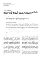
intensity (7)byafactorF. Figure 1 displays XRD intensity
Table 1: Values of parameters used in (6) to compute synthetic
XRD intensity profiles. The wavelength and the f.c.c. bulk lattice
constant were set to λ
= 0.15418 nm and a
f.c.c.
= 0.40786 nm, re-
spectively.
Parameter X = CX= IX= D
ξ
X
5.0 5.0 5.0
s
X
0.3 0.3 0.3
n

0
X
4.0 4.0 6.0
Ω
X
1.0 1.0 1.0
Ξ
X
1.0 1.0 1.0
w
X
0.5 0.5 0.5
0
1000
2000
3000
4000
5000
6000
0.20.30.40.50.60.70.80.91
ϑ (rad)
XRD intensity (AU)
Figure 1: Synthetic XRD intensity profiles as a function of the scat-
tering angle. From the upper to the lower profile, the NSR increases
from 2% to 5% (see Figure 2 and text for details).
profiles with increasing NSRs. They were obtained by setting
λ
= 0.15418 nm and a
f.c.c.
= 0.40786 nm in (6). The set of

parameters used to compute the synthetic profiles are sum-
marized in Ta ble 1 . Figure 2 shows the NSR of the synthetic
profiles as a function of the scaling factor F ranging from 0
to 2. This range contains the NSR values usually measured in
experimental profiles.
We also considered real data in order to validate our
method. Three different samples were prepared with resul-
tant mean diameters of 2.0, 3.2, and 4.1 nm, respect ively
(as measured by transmission electron microscope). The size
distributions were approximately characterized by the same
full width at half-maximum (
≈ 1 nm) for all three systems.
4. NUMERICAL RESULTS
Noisy synthetic XRD patterns were generated correspond-
ing to nanocrystalline samples of increasing size from 2 to
4 nm, and Poisson-distributed noise with increasing NSR
from 2% to 10%. The HLSVD-PRO filter was then applied
to the noisy synthetic XRD signals in order to study their
4 EURASIP Journal on Advances in Signal Processing
Table 2: Measure E (see (3)) of the filter performance as a function
of the o rder K of the filter. The synthetic XRD intensity data refer to
different sample sizes and NSRs. The best performance corresponds
to the order K reported in the middle row of each NSR value.
2nm 3nm 4nm
NSR = 10%
K − 21.86 ±0.16 1.25 ±0.09 1.67 ±0.10
K = 92.49 ±0.16 2.34 ±0.20 1.89 ±0.19
K +2 2.43 ± 0.42 2.28 ±0.21 1.73 ±0.18
NSR = 5%
K − 22.17 ±0.18 1.81 ±0.16 1.52 ±0.11

K = 11 2.34 ±0.18 1.87 ±0.16 1.56 ±0.12
K +2 2.22 ± 0.28 1.87 ±0.16 1.48 ±0.09
NSR = 2%
K − 21.80 ±0.21 1.37 ±0.32 1.13 ±0.14
K = 15 1.89 ±0.28 1.54 ±0.39 1.25 ±0.06
K +2 1.86 ± 0.18 1.46 ±0.38 1.18 ±0.09
0
0.05
0.1
0.15
0.2
0.25
00.20.40.60.811.21.41.61.82
Scaling factor F
NSR
Figure 2: NSR as a function of the factor F,seetextfordetails.The
horizontal line separ ates the NSR values above and below F
= 1.
properties under controlled conditions. Figure 3 displays an
example of application of the HLSVD-PRO filter. A noisy
synthetic XRD intensity profile is shown at the top of the
figure. It corresponds to X-ray scattering from an Au sam-
ple having a 3 nm size with a Poisson-like noise with NSR
=
10%. The filtered signal shown in the middle of the figure was
obtained by setting K
= 9 in the HLSVD-PRO filter. In the
following (see Ta ble 2 for results), we discuss in more detail
the performance of the method when the values K
= 7and

K
= 11 are used. This value was estimated according to the
criterion illustrated in Section 2.Thevaluesofλ
k
were plot-
ted by first sorting frequencies f
k
in ascendant order. Specif-
ically, a transition from high to small λ
k
was observed at fre-
quency f
K
= 35 rad
−1
, which represents the Kth frequency
in the set of the sorted frequencies starting from the smallest
one. For a comparison, the discrete Fourier transform (DFT)
of the noisy synthetic XRD signal is reported at the bottom
of Figure 4. Again, a phenomenon of transition from high to
small singular values occurs in the same region of the spec-
trum, as observed at the top of the figure. However, the tran-
0
200
400
0.20.30.40.50.60.70.80.91
ϑ (rad)
XRD intensity (AU)
(a)
0

200
400
0.20.30.40.50.60.70.80.91
ϑ (rad)
XRD intensity (AU)
(b)
−50
0
50
0.20.30.40.50.60.70.80.91
ϑ (rad)
XRD intensity (AU)
(c)
Figure 3: Three nm Au synthetic sample: (a) noisy (NSR = 10%)
synthetic XRD intensity profile as a function of the scattering angle
ϑ; (b) filtered XRD intensity profile; (c) difference between mea-
sured and filtered profiles.
sition frequency is much more difficult to localize than in
the HLSVD-PRO filter case. The same behavior is observed
when using the WF filter. This makes troublesome the appli-
cation of DFT and WF filters to clean noisy XRD data. It is
worth noting that this difference between the HLSVD-PRO
and Fourier-frequency-based filters is relevant when the fil-
ter is intended to b e used during interactive XRD data anal-
ysis. In this case, the successful application of an easy-to-use
blackbox filter becomes crucial.
Coming back to Figure 3, the difference between the val-
ues of noisy and filtered profiles is shown at the bottom.
To quantify the performance of the filter, the filtered signal
was compared with the noiseless synthetic XRD signal (see

Figure 5). For the sake of completeness, we also report in
Figure 5 the residue between the noiseless and the filtered
signals. This can be done only with synthetic signals as ex-
perimental XRD data without noise are not available. To give
a statistical significance to these measures a Monte Carlo
experiment was carried out. More precisely, the HLSVD-
PRO was applied to 1000 noisy synthetic profiles generated
by considering samples of the same size undergoing differ-
ent NSRs. For each filtered profile, the filter per formance
measure E,definedin(3), was estimated by calculating the
mean value and the standard deviation. For each sample size
and NSR, the mean and standard deviation are obtained
using 1000 synthetic XRD intensity profiles with different
M. Ladisa et al. 5
2
2.5
3
3.5
4
4.5
5
0 50 100 150 200 250
f (rad
−1
)
log |λ
i
|
(a)
0

1
2
3
4
5
0 50 100 150 200 250
f (rad
−1
)
|DFT{I(ϑ)}|
(b)
Figure 4: Three nm Au synthetic sample with NSR = 10%: (a)
amplitude of eigenvalues λ
k
versus frequency f
k
, k = 1, , r;(b)
portion of the DFT amplitude spectrum of the noisy synthetic XRD
intensity profile. Both plots refer to the XRD intensity profile shown
at the top of Figure 3.
noise realizations having the same NSR. The sensitivity to the
number K of sinusoids of the HLSVD-PRO filter was also
studied. This number was slightly varied around the opti-
mal K value selected by using the threshold criterion. The
performance results were compared in order to validate the
choice of the optimal K value. In particular, K was increased
and decreased by 2, as discussed in Section 1. The results of
such a comparison are summarized in Tab le 2 and they show
that the proposed threshold criterion provides the value of K
corresponding to the best performance of the HLSVD-PRO

filter.
The filter was also applied to real XRD intensity profiles
of Au samples of sizes 2, 3.2, and 4.1 nm. Figure 6 shows at
top the profile of a 3.2 nm Au sample with NSR
= 2.3%.
Thelatteriscomputedas
σ/I,whereσ and I are vec-
tors with the measured error and the intensity values, re-
spectively. Since in the case of XRD signals, the noise fol-
lows the Poisson distribution, σ is given by
√
I. T he result
obtained by HLSVD-PRO is displayed in the middle of the
figure. At bottom, the plot of singular values is depicted ver-
sus the frequency. Components with a frequency higher than
f
K
= 34 rad
−1
, due to noise, were removed. Denoising a real
XRD profile of 500 intensity data samples, as typical ones
used in the present study, requires about 11 seconds, using
Matlab 7 on a machine with an Intel Xeon 2.80 GHz proces-
sor and a 512 KB cache size.
Finally, as a matter of comparison, we applied two well-
known parametric algorithms that are commonly used for
spectral analysis: MUSIC and ESPRIT [17]. Such methods
are generally expected to be more effective spectral tools
compared to DFT since they rely on the use of a model func-
0

100
200
300
400
0.20.30.40.50.60.70.80.91
ϑ (rad)
XRD intensity (AU)
(a)
−50
0
50
0.20.30.40.50.60.70.80.91
ϑ (rad)
XRD intensity residue (AU)
(b)
Figure 5: Three nm Au synthetic sample with NSR = 10%: (a)
noiseless synthetic XRD intensity profile as a function of the scatter-
ing angle ϑ;(b)difference between noiseless and filtered (see middle
plot of Figure 3) profiles.
tion. However, in the present case where the signal is better
modelled with damped sinusoids, the aforementioned meth-
ods are not able to correctly filter the signal. This limitation
comes from the use of prescribed model functions that do
not account for damping. Extensive simulation studies by us-
ing synthetic as well as real data show that MUSIC and ES-
PRIT fail. For instance, for the real XRD intensity reported
in Figure 6, we computed the residue-to-signal ratio (RSR).
We obtain the following results: RSR
= 54% (ESPRIT), 51%
(MUSIC), 2% (HLSVD).

5. CONCLUSIONS
A filter based on the HLSVD-PRO method has been pre-
sented. It has been applied to filter XRD patterns of nan-
ocluster powders. The filter performance has been studied
on synthetic and real XRD patterns w ith different NSRs. Re-
sults show that the proposed filter is robust and computa-
tionally efficient. A further advantage is its user-friendliness
that makes it a useful blackbox tool for the processing of XRD
data.
APPENDICES
HSVD is a subspace-based parameter estimation method in
which the noisy signal is arranged in a Hankel matrix H.Its
SVD allows to compute a “signal” subspace and a “noise”
subspace. In fact, if H is constructed from a noiseless sig-
nal, the data matrix H hasexactlyrankequaltoK, the num-
ber of exponentials that models the underlying signal. Due
to the presence of the noise, H becomes a full-rank matrix.
6 EURASIP Journal on Advances in Signal Processing
0
2
4
6
×10
3
0.20.30.40.50.60.70.80.91
ϑ (rad)
XRD intensity (AU)
(a)
0
2

4
6
×10
3
0.20.30.40.50.60.70.80.91
ϑ (rad)
XRD intensity (AU)
(b)
3
4
5
6
0 50 100 150 200 250
f (rad
−1
)
log |λ
i
|
(c)
Figure 6: Au real sample of 3.2 nm: (a) noisy (NSR = 2.3%) XRD
intensity profile as a function of the scattering angle ϑ; (b) filtered
XRD intensity profile; (c) amplitudes of eigenvalues λ
k
versus fre-
quency f
k
, k = 1, , q.
However, as long as the SNR of the sig nal is not too low, one
can still define the “numerical” r ank being approximately

equal to K. Then, the “signal” subspace is found by truncat-
ing the SVD of the matrix H to rank K.
In the following subsections, the method will be derived
in the context of linear algebra.
A. HSVD: THE ALGORITHM
The N data points defined in (1) are arranged into a Hankel
matrix H of dimensions L
× M,withL + M = N +1and
L
 N/2,
H
L×M
=
⎡
⎢
⎢
⎢
⎢
⎢
⎣
I
0
I
1
··· ··· I
M−1
I
1
I
2

··· ··· I
M
.
.
.
.
.
.
.
.
.
.
.
.
.
.
.
I
L−1
I
L−2
··· ··· I
N−1
⎤
⎥
⎥
⎥
⎥
⎥
⎦

L×M
. (A.1)
The SVD of the Hankel matrix is computed as
H
L×M
= U
L×L
Σ
L×M
V
H
M
×M
,(A.2)
where Σ
= diag{λ
1
, λ
2
, , λ
r
}, λ
1
≥ λ
2
≥ ··· ≥ λ
r
≥ 0,
r
= min(L, M), U and V are orthogonal matrices, and the

superscript H denotes the Hermitian conjugate. The SVD is
computed by using the Lanczos bidiagonalization algorithm
with partial reorthogonalization [18]. This algorithm com-
putes two matrix-vector products at each step. Exploiting the
structure of the matrix (A.1) by using the FFT, the latter com-
putation requires O((L+M)log
2
(L+M)) rather than O(LM).
In order to obtain the “signal” subspace, the matrix H is
truncated to a matrix H
K
of rank K,
H
K
= U
K
Σ
K
V
H
K
,(A.3)
where U
K
, V
K
,andΣ
K
are defined by taking the first K
columns of U and V, and the K

× K upper-left matrix of
Σ, respec tively. The way of choosing K is described at the be-
ginning of Section 4. As a subsequent step, the least-squares
solution E of the following overdetermined set of equations
is computed as
U
(top)
K
 U
(bottom)
K
E,(A.4)
where U
(bottom)
K
and U
(top)
K
are derived from U
K
by deleting its
last and fi rst rows, respectively. Equation (A.4)followsfrom
the shift-invariance property holding for the Vandermonde
decomposition of the Hankel matrix H [7]. The K eigenval-
ues
z
k
of the matrix E are used to estimate the frequencies

f

k
and the damping factors

d
k
of the model damped sinusoids
from the relationship
z
k
= exp

−

d
k
+ i2π

f
k

Δϑ

,(A.5)
as

d
k
=−



log


z
k

Δϑ
,

f
k
=


log


z
k

(2πΔϑ)
,
(A.6)
with k
= 1, , K.
B. HSVD: NOISELESS DATA
Arrange the N noiseless data points I
0
n
defined in (1)ina

Hankel matrix H of dimensions L
×M,withL and M greater
than K and N
= L + M − 1,
H
=
⎡
⎢
⎢
⎢
⎢
⎢
⎣
I
0
0
I
0
1
··· I
0
M
−1
I
0
1
I
0
2
··· I

0
M
.
.
.
.
.
.
.
.
.
.
.
.
I
0
L
−1
I
0
L
−2
··· I
0
N
−1
⎤
⎥
⎥
⎥

⎥
⎥
⎦
. (B.1)
The model of (1) can be rewritten in terms of complex am-
plitudes c
k
and signal poles z
k
as follows:
I
0
n
=
K

k=1
c
k
z
n
k
, n = 0, , N −1, (B.2)
where c
k
= a
k
exp (iϕ
k
)exp(−


d
k
+ i2π

f
k
)ϑ
0
and z
k
=
exp(−

d
k
+ i2π

f
k
)Δϑ. Using this model function, the Hankel
M. Ladisa et al. 7
matrix H can be factorized as follows:
H
=
⎡
⎢
⎢
⎢
⎢

⎢
⎣
11··· 1
z
1
z
2
··· z
K
.
.
.
.
.
.
.
.
.
.
.
.
z
L−1
1
z
L−1
2
··· z
L−1
K

⎤
⎥
⎥
⎥
⎥
⎥
⎦
⎡
⎢
⎢
⎢
⎢
⎢
⎣
c
1
0 ··· 0
0 c
2
··· 0
.
.
.
.
.
.
.
.
.
.

.
.
00
··· c
K
⎤
⎥
⎥
⎥
⎥
⎥
⎦
×
⎡
⎢
⎢
⎢
⎢
⎢
⎣
11··· 1
z
1
z
2
··· z
K
.
.
.

.
.
.
.
.
.
.
.
.
z
M−1
1
z
M−1
2
··· z
M−1
K
⎤
⎥
⎥
⎥
⎥
⎥
⎦
T
= SCT
T
.
(B.3)

This factorization is called Vandermonde decomposition and
from it the signal parameters can immediately be derived. A
well-known algorithm to directly compute the Vandermonde
decomposition is available in the literature and is called
Prony’s method [19–22]. Here, a more reliable approach,
based on an indirect computation of the parameters, is
adopted. This approach is described below. From (B.3), it can
be easily proved that the matrix S satisfies the so-called shift-
invariance property, that is,
S
↑
= S
↓
Z,(B.4)
where S
↑
and S
↓
are derived from S by deleting its first and last
rows, respectively, and Z is a K
× K complex diagonal matrix
with entries equal to the K signal poles z
k
, k = 1, , K.The
rank of the matr ix H is equal to K, and thus, its SVD has the
following form:
H
= UΣV
H
=


U
K
U
2


Σ
K
0
00


V
K
V
2

H
= U
K
Σ
K
V
H
K
,
(B.5)
where U
K

∈ C
L×K
, U
2
∈ C
L×(L−K)
, Σ
K
∈ C
K×K
, V
K
∈ C
M×K
,
V
2
∈ C
M×(M−K)
. From the comparison of (B.3)and(B.5), it
follows that S and U
K
span the same column space, and hence
are equal up to a multiplication by a nonsingular matrix Q
∈
C
K×K
, that is,
U
K

= SQ. (B.6)
Using (B.6), the shift-invariance propert y of (B.4)becomes
U
↑
K
= U
K↓
Q
−1
ZQ. (B.7)
The matrix Q
−1
ZQ can be determined as the least-squares
solution of (B.7). Several reliable and efficient algorithms are
available in the literature and they exploit well-known alge-
braic tools such as the QR decomposition, the SVD decom-
position, and so forth. The reader is referred to [12, 23],
where an exhaustive overview on the computation of the
least-squares solution of a system of equations is provided.
Since the eigenvalues of Q
−1
ZQ and Z are equal, the signal
poles are easily derived as

z
k

K
k
=1

= eig

Q
−1
ZQ

= eig(Z), (B.8)
where the function eig(
·) determines the eigenvalues of the
matrix between br a ckets.
From the signal poles, frequency and damping factors
are estimated. By filling in these estimates into the model
function (B.2), a new system of equations is obtained with
unknowns equal to the complex variables c
k
. Its solution pro-
vides estimates for the amplitudes and the phases.
C. HSVD: NOISY DATA
When noise affects the data, as in real MRS signals, rela-
tion (B.5) no longer holds. Although no exact solution of
the shift-invariance property exists, if the noise is small com-
pared to the signal, H can be approximated by the truncated
SVD, that is,
H
= UΣV
H
≈ U
K
Σ
K

V
H
K
= H
K
,(C.1)
where U
K
and V
K
are the first K columns of U and V,re-
spectively, and Σ
K
is the K ×K upper-left submatrix of Σ.
The matrix H
K
has rank K but its Hankel structure has
been destroyed by the truncation of the SVD. Therefore,
there exists no exact solution of the system in (C.1). However,
estimates of the signal poles can still be obtained by solving
the aforementioned system in an LS sense and the signal pa-
rameters can be derived from such estimates as in the noise-
less case. Further details about the derivation of HSVD can
be found in [7, 24].
ACKNOWLEDGMENTS
The authors thank A. Cervellino, C. Giannini, and A. Guagl-
iardi for kindly providing us with experimental XRD data.
REFERENCES
[1] B. Mierzwa and J. Pielaszek, “Smoothing of low-intensity noisy
X-ray diffr action data by Fourier filtering: application to sup-

ported metal catalyst studies,” JournalofAppliedCrystallogra-
phy, vol. 30, no. 5, pp. 544–546, 1997.
[2] A. Hieke and H D. D
¨
orfler, “Methodical developments for X-
ray diffraction measurements and data analysis on lyotropic
liquid crystals applied to K-soap/glycerol systems,” Colloid and
Polymer Science, vol. 277, no. 8, pp. 762–776, 1999.
[3] M. Schmidt, S. Rajagopal, Z. Ren, and K. Moffat, “Appli-
cation of singular value decomposition to the analysis of
time-resolved macromolecular X-ray data,” Biophysical Jour-
nal, vol. 84, no. 3, pp. 2112–2129, 2003.
[4] S. Rajagopal, M. Schmidt, S. Anderson, H. Ihee, and K. Mof-
fat, “Analysis of experimental time-resolved crystallographic
data by singular value decomposition,” Acta Crystallographica
Section D, vol. 60, no. 5, pp. 860–871, 2004.
[5] E. E. Aubanel and K. B. Oldham, “Fourier smoothing without
the fast Fourier transform,” By te, vol. 10, no. 2, pp. 207–222,
1985.
[6] C. Wooff, “Smoothing of data by least squares fitting,” Com-
puter Physics Communications, vol. 42, no. 2, pp. 249–251,
1986.
[7] H. Barkhuijsen, R. de Beer, and D. van Ormondt, “Improved
algorithm for noniterative time-domain model fitting to expo-
nentially damped magnetic resonance signals,” Journal of Mag-
netic Resonance, vol. 73, no. 3, pp. 553–557, 1987.
8 EURASIP Journal on Advances in Signal Processing
[8] T. Laudadio, N. Mastronardi, L. Vanhamme, P. van Hecke,
and S. van Huffel, “Improved Lanczos algorithms for black-
box MRS data quantitation,” Journal of Magnetic Resonance,

vol. 157, no. 2, pp. 292–297, 2002.
[9] D. J. Wales, “Structure, dynamics, and thermodynamics of
clusters: t ales from topographic potential surfaces,” Science,
vol. 271, no. 5251, pp. 925–929, 1996.
[10] R. W. Siegel, E. Hu, D. M. Cox, et al., “Nanostructure Sci-
ence and Technolgy. A Worldwide Study,” The Interagency
Working Group on NanoScience, Engineering and Technolgy,
/>[11] D. Zanchet, M. B. D. Hall, and D. Ugarte, “Structure popula-
tion in thioi-passivated gold nanoparticles,” JournalofPhysical
Chemistry B, vol. 104, no. 47, pp. 11013–11018, 2000.
[12] G. H. Golub and C. Reinsch, “Singular value decomposition
and least squares solutions,” Numerische Mathematik, vol. 14,
no. 5, pp. 403–420, 1970.
[13] E.Anderson,Z.Bai,C.Bischof,etal.,LAPACK Users’ Guide,
SIAM, Philadelphia, Pa, USA, 1995.
[14] R. A. Young, The Rietvel Method, Oxford University Press, New
York, NY, USA, 1993.
[15] A. Cervellino, C. Giannini, and A. Guagliardi, “Determina-
tion of nanoparticle structure ty pe, size and strain distri-
bution from X-ray data for monatomic f.c.c derived non-
crystallographic nanoclusters,” JournalofAppliedCrystallog-
raphy, vol. 36, no. 5, pp. 1148–1158, 2003.
[16] J. R. Taylor, An Introduction to Error Analysis: The Study of
Uncertainties in Physical Measurements, University Scientific
Books, Sausalito, Calif, USA, 1997.
[17] P. Stoica and R. Moses, Introduction to Spectral Analysis,
Prentice-Hall, Upper Saddle River, NJ, USA, 1997.
[18] H. D. Simon, “The Lanczos algorithm with partial reorthogo-
nalization,” Mathematics of Computation, vol. 42, no. 165, pp.
115–142, 1984.

[19] S. L. Marple, Digital Spectral Analysis with Applications,
Prentice-Hall, Englewood Cliffs, NJ, USA, 1987.
[20] G. Golub and V. Pereyra, “Separable nonlinear least squares:
the variable projection method and its applications,” Inverse
Problems, vol. 19, no. 2, pp. R1–R26, 2003.
[21] B. J. C. Baxter and A. Iserles, “On approximation by expo-
nentials,” Annals of Numerical Mathematics, vol. 4, pp. 39–54,
1997, The heritage of P. L. Chebyshev: a Festschrift in honor of
the 70th birthday of T. J. Rivlin, hskip 1em plus 0.5em minus
0.4em.
[22] G. Beylkin and L. Monzon, “On approximation of functions
by exponential sums,” Applied and Computational Harmonic
Analysis, vol. 19, no. 1, pp. 17–48, 2005.
[23] A. Bjoirck, Numerical Methods for Least Squares Problems,
SIAM, Philadelphia, Pa, USA, 1996.
[24] S. Y. Kung, K. S. Arun, and D. V. Bhaskar Rao, “State-space and
singular-value decomposition-based approximation methods
for the harmonic retrieval problem,” Journal of the Optical So-
ciety of America, vol. 73, no. 12, pp. 1799–1811, 1983.
M. Ladisa received the Laurea and Ph.D. degrees in physics from
the University of Bari, Bari, Italy, in 1997 and 2001, respectively. He
is currently a Researcher with the Istituto di Cristallografia (IC),
National Research Council (CNR), Bari, Italy.
A. Lamura received the Laurea and Ph.D.
degrees in physics from the University of
Bari, Bari, Italy, in 1994 and 2000, respec-
tively. He is currently a Researcher with
the Istituto per le Applicaizoni del Calcolo
(IAC), National Research Council (CNR),
Bari, Italy.

T. Laudadio received the Laurea degree in
mathematics from the University of Bari,
Bari, Italy, in 1992, and the Ph.D. degree in
electrical engineering from the Katholieke
Universiteit Leuven, Leuven, Belgium, in
2005. She is currently a Research Fellow
with the Istituto di Studi sui Sistemi Intel-
ligenti per l’Automazione (ISSIA), National
Research Council (CNR), Bari, Italy.
G. Nico received the Laurea and Ph.D. degrees in physics from the
University of Bari, Bari, Italy, in 1993 and 1999, respectively. He
is currently a Researcher with the Istituto per le Applicaizoni del
Calcolo (IAC), National Research Council (CNR), Bari, Italy.