Báo cáo hóa học: "NEW CLASSES OF GENERALIZED INVEX MONOTONICITY" docx
Bạn đang xem bản rút gọn của tài liệu. Xem và tải ngay bản đầy đủ của tài liệu tại đây (656.54 KB, 19 trang )
NEW CLASSES OF GENERALIZED INVEX MONOTONICITY
B. XU AND D. L. ZHU
Received 26 December 2004; Accepted 16 August 2005
This paper introduces new classes of generalized invex monotone mappings and invex co-
coercive mappings. Their differential property and role to analyze and solve variational-
like inequality problem are presented.
Copyright © 2006 B. Xu and D. L. Zhu. This is an open access article distributed under
the Creative Commons Attribution License, which permits unrestricted use, distribution,
and reproduction in any medium, provided the original work is properly cited.
1. Introduction
Variational inequalities theory has been widely used in many fields, such as econom-
ics, physics, engineering, optimization and control, transport ation [1, 4]. Like convexity
to mathematical programming problem (MP), monotonicity plays an important role in
solving variational inequality (VI). To investigate the variational inequality, many kinds
of monotone mappings have been introduced in the literature, see Karamardian and
Schaible [5], for example. In [2], Crouzeix, et al. introduced the concepts of monotone
plus mappings and proved the important role in the convergence of cutting-plane method
for solving variational inequities. In [14], Zhu and Marcotte introduced the classes of gen-
eralized cocoercive mapping and related them to classes previously introduced. Zhu and
Marcotte [15] investigate iterative schemes for solving nonlinear variational inequalities
under cocoercive assumption.
Variational-like inequality problem (VLIP) or prevariational inequalities (PVI) is more
general problem than VIP, which is first introduced by Parida et al. [9]. Invex monotonic-
ity, which is a generalization of classical monotonicity, is investigated widely by many
researchers for studying invex function, which is generalization of convex function [6–
8, 12, 13], and solving VLIP [3, 9–11]. Ruiz-Garz
´
on et al. [10] introduce some generalized
invex monotonicity which are also discussed in [13], mentioned as generalized invariant
monotonicity.
The purpose of this paper is to introduce new classes of generalized invex monotone
plus mappings and generalized invex cocoercive mappings and analyze their properties
and relationships with respect to other concepts of invex monotonicity. Some examples,
Hindawi Publishing Corporation
Journal of Inequalities and Applications
Volume 2006, Article ID 57071, Pages 1–19
DOI 10.1155/JIA/2006/57071
2 New classes of generalized invex monotonicity
counterexamples, and theoretical results are offered. These concepts allow the develop-
ment of the convergent algorithm to solving VLIP and characterization of the solution
set of VLIP. This paper will be organized as follows: for easy of reference, the next section
regroups all definitions of generalized monotonicity, invexity, and invex monotonicity re-
quired in our study; in Sections 3 and 4, we introduce the new class of generalized invex
monotone plus mappings, and generalized invex cocoercive mappings respectively. We
analyze the differential property of these new generalized invex monotone mappings in
Section 5. We discuss the usefulness of the new concepts of generalized invex monotonic-
ity for VLIP in Section 6. The concluding section concludes.
2. Preliminaries
Let K be a nonempty subset of
R
n
, η : K ×K → R
n
(K ⊂ R
n
), let F be a vector-valued
function from K into
R
n
,andlet f be a differentiable function from K to R.
Karamardian introduced some monotone mappings in [5]. In [2], some new mono-
tonicity, such as monotone
+
and pseudomonotone
+
are introduced and applied to cut-
ting-plane methods for solving variational inequalities.
Definit ion 2.1 [2]. F is said to be
(i) monotone
+
(M
+
)onK if it is monotone on K and ∀x, y ∈K,
F(y) −F(x), y −x
=
0 =⇒ F(y) =F(x); (2.1)
(ii) monotone
+
∗
(M
+
∗
)onK if it is monotone on K and ∀x, y ∈K,
F(y), y −x
=
F(x), y −x
=
0 =⇒ F(y) =F(x); (2.2)
(iii) monotone
∗
(M
∗
)onK if it is monotone on K and ∀x, y ∈K,
F(y), y −x
=
F(x), y −x
=
0 =⇒ ∃k>0, such that F(y) =kF(x); (2.3)
(iv) pseudomonotone
+
(PM
+
)onK if it is pseudomonotone on K and ∀x, y ∈K,
F(y) −F(x), y −x
=
0 =⇒ F(y) =F(x); (2.4)
(v) pseudomonotone
+
∗
(PM
+
∗
)onK if it is pseudomonotone on K and ∀x, y ∈K,
F(y), y −x
=
F(x), y −x
=
0 =⇒ F(y) =F(x); (2.5)
(vi) pseudomonotone
∗
(PM
∗
)onK if it is pseudomonotone on K and ∀x, y ∈K,
F(y), y −x
=
F(x), y −x
=
0 =⇒ ∃k>0, such that F(y) =kF(x). (2.6)
Some relationships among the various generalized monotonicity can be represented
by Figure 2.1 (see [2] for more details).
The cocoercive and generalized cocoercive mappings are introduced in [14]. The role
of cocoercivit y for solving variational inequalities is investigated in [15].
B. Xu and D. L. Zhu 3
PM
+
PseudomonotonePM
+
∗
PM
∗
M
+
M
+
∗
M
∗
Monotone
Figure 2.1. Relationships between the monotone plus classes.
Strictly pseudomonotone PseudomonotoneStrictly pseudococoercive Pseudococoercive
Strictly monotone Strictly cocoercive Cocoercive Monotone
Figure 2.2. Relationships between generalized cocoercive mappings.
Definit ion 2.2 [14]. F is said to be
(i) cocoercive on K if there exists α>0, for any x, y
∈ K,
F(y) −F(x), y −x
≥
α
F(y) −F(x)
2
; (2.7)
(ii) strictly cocoercive on K if there exists α>0, for any distinct x, y ∈K,
F(y) −F(x), y −x
>α
F(y) −F(x)
2
; (2.8)
(iii) pseudococoercive on K if there exists α>0, for any distinct x, y ∈ K,
F(x), y −x
≥
0 =⇒
F(y), y −x
≥
α
F(y) −F(x)
2
; (2.9)
(iv) strictly pseudococoercive on K if there exists α>0, for any distinct x, y ∈ K,
F(x), y −x
≥
0 =⇒
F(y), y −x
>α
F(y) −F(x)
2
. (2.10)
We can describe their relationships as shown in Figure 2.2 (see [14] for more details).
Invex function and generalized invex function are investigated by many authors, which
are generalizations of convex function and generalized convex function [6–8, 12, 13].
Definit ion 2.3 [10]. f is said to be
(i) invex (IX) on K with respect to η if for any x, y
∈ K,
f (y) − f (x) ≥
∇f (x),η(y,x)
; (2.11)
(ii) strictly invex (SIX) on K with respect to η if for any distinct x, y
∈ K,
f (y) − f (x) >
∇
f (x),η(y,x)
; (2.12)
(iii) strongly invex (SGIX) on K with respect to η if there exists α>0, such that
f (y)
− f (x) ≥
∇f (x),η(y,x)
+ α
η(y,x)
2
, ∀x, y ∈K; (2.13)
4 New classes of generalized invex monotonicity
SGPIX SPIX PIX QIX
SGIX SIX IX
Figure 2.3. Relationships between the generalized invex functions.
(iv) pseudoinvex (PIX) on K with respect to η if for any x, y ∈ K,
∇
f (x),η(y,x)
≥
0 =⇒ f (y) − f (x) ≥0; (2.14)
(v) strictly pseudoinvex (SPIX) on K with respect to η if for any distinct x, y
∈ K,
∇
f (x),η(y,x)
≥
0 =⇒ f (y) − f (x) > 0; (2.15)
(vi) strongly pseudoinvex (SGPIX) on K with respect to η if there exists α>0, such that
∇
f (x),η(y,x)
≥
0 =⇒ f (y) ≥ f (x)+α
η(y,x)
2
, ∀x, y ∈ K; (2.16)
(vii) quasi-invex (QIX) on K with respect to η if for any x, y
∈ K,
f (y)
− f (x) ≤0 =⇒
∇
f (x),η(y,x)
≤
0. (2.17)
From the definitions, we can establish their relationships as shown in Figure 2.3.
In [10], the definitions of generalized invex monotonicity are offered, which generalize
generalized monotonicity established by Karamardian [5].
Definit ion 2.4 [10]. F is said to be
(i) invex monotone (IM) on K with respect to η if for any x, y
∈ K,
F(y) −F(x), η(y,x)
≥
0; (2.18)
(ii) strictly invex monotone (SIM) on K with respect to η if for any distinct x, y
∈ K,
F(y) −F(x), η(y,x)
> 0; (2.19)
(iii) strongly invex monotone (SGIM) on K with respect to η if there exists β>0, such
that
F(y) −F(x), η(y,x)
≥
β
η(y,x)
2
, ∀x, y ∈K; (2.20)
(iv) pseudoinvex monotone (PIM) on K with respect to η if for any x, y
∈ K,wehave
F(x), η(y,x)
≥
0 =⇒
F(y),η(y, x)
≥
0; (2.21)
(v) str ictly pseudoinvex monotone (SPIM) on K with respect to η if for any distinct
x, y
∈ K,
F(x), η(y,x)
≥
0 =⇒
F(y),η(y, x)
> 0; (2.22)
B. Xu and D. L. Zhu 5
SGPIM SPIM PIM QIM
SGIM SIM IM
Figure 2.4. Relationships between the invex monotonicity classes.
(vi) strongly pseudoinvex monotone (SGPIM) on K with respect to η if there exists β>
0, such that
F(x), η(y,x)
≥
0 =⇒
F(y),η(y, x)
≥
β
η(y,x)
2
, ∀x, y ∈K; (2.23)
(vii) quasi-invex monotone (QIM) on K if for any x, y
∈ K,
η(y,x)
T
F(x) > 0 =⇒ η(y, x)
T
F(y) ≥0. (2.24)
From the definitions, their relationships are described as shown in Figure 2.4.
Remark 2.5. From the definition, we can see that every (generalized) monotone mapping
is (generalized) invex monotone mapping with η(x, y)
= x − y, but the converse is not
necessarily true. Examples and counterexamples can be found in [10, 13].
Remark 2.6. When η(x, y)+η(y,x)
= 0, invariant monotonicity defined in [13]isequiv-
alent to invex monotonicity.
3. New class of generalized invex monotone mappings
In this section, we will present the definitions of (pseudo) invex monotone plus map-
pings, and so forth, and discuss their relationships by examples and counterexamples.
3.1. Invex monotone plus mappings
Definit ion 3.1. F is said to be
(i) invex monotone
+
(IM
+
)onK with respect to η if it is invex monotone on K with
respect to η and, for any x, y
∈ K,
F(y) −F(x), η(y,x)
=
0 =⇒ F(y) =F(x); (3.1)
(ii) invex monotone
+
∗
(IM
+
∗
)onK with respect to η if it is invex monotone on K with
respect to η and, for any x, y
∈ K,
F(y),η(y, x)
=
F(x), η(y,x)
=
0 =⇒ F(y) =F(x); (3.2)
(iii) invex monotone
∗
(IM
∗
)onK with respect to η if it is invex monotone on K with
respect to η and, for any x, y
∈ K,
F(y),η(y, x)
=
F(x), η(y,x)
=
0 =⇒ ∃k>0, such that F(y) =kF(x). (3.3)
6 New classes of generalized invex monotonicity
Remark 3.2. (i) Every M
+
(M
+
∗
,M
∗
)mappingisIM
+
(IM
+
∗
,IM
∗
) mapping with η(x, y) =
x − y, but the converse is not necessarily true.
(ii) According to the above definitions, we have SIM
⇒ IM
+
⇒ IM
+
∗
⇒IM
∗
⇒IM, but
the converse is not necessarily true.
Example 3.3. Let F(x)
=
sinx
1
sinx
2
, η(x, y) =
sinx
2
−sin y
2
sin y
1
−sinx
1
.Obviously,F(x)isIMonR
2
with
respect to η.Letx
= (π/2,π/2)
T
, y = (−π/2,−π/2)
T
,
F(y),η(y, x)
=
F(x), η(y,x)
=
0, (3.4)
but there is no k>0suchthatF(y)
= kF(x). This implies that F(x) is not IM
∗
on R
2
with
respect to η.
Example 3.4. Let F(x)
=
sinx
1
sinx
2
, η(x, y) =
sinx
2
−sin y
2
sin y
1
−sinx
1
,andK = (0,π) ×(0,π). By defi-
nition, F(x)isIM
∗
on K with respect to η.Letx = (π/2,π/2)
T
, y = (5π/6,5π/6)
T
,we
have
F(y),η(y, x)
=
F(x), η(y,x)
=
0, (3.5)
but F(y)
= F(x), which means F(x) is not IM
+
∗
on K with η. Meanwhile, we have
F(y) −F(x), y −x
=−
π
3
< 0. (3.6)
Therefore F(x) is not M
∗
on K.
Example 3.5. Let F(x)
=
sinx
2
−sinx
1
−sinx
2
, η(x, y) =
sinx
2
−sin y
2
sin y
1
−sinx
1
,andK = (0,π) ×(0,π). We
have
F(y) −F(x), η(y,x)
=
sin y
2
−sinx
2
2
= 0 (3.7)
if and only if sinx
2
= sin y
2
. Furthermore, with the condition
F(x), η(y,x)
=
sinx
2
−sinx
1
sinx
2
−sin y
2
+ sinx
2
sinx
1
−sin y
1
=
0, (3.8)
we have sinx
1
= sin y
1
. It shows that F(x)isIM
+
∗
on K with respect to η.
Let x
= (π/2,π/2)
T
, y = (π/6,π/2)
T
,wehave
F(y) −F(x), η(y,x)
=
0, (3.9)
but F(y)
= F(x). This implies F(x)isnotIM
+
on K with respect to η. Meanwhile, F(x)is
not M
+
∗
on K, since
F(y) −F(x), y −x
=−
π
6
< 0. (3.10)
Example 3.6. Let F(x)
= cos
2
x, η(x, y) =sin
2
y −sin
2
x,andK =(−π/2,π/2). Obviously,
F(x)isIM
+
on K with respect to η, but not SIM on K with η, since
F(y) −F(x), η(y,x)
=
0, if x =−y = 0. (3.11)
B. Xu and D. L. Zhu 7
Meanwhile, F(x) is not M
+
yet, since
F(y) −F(x), y −x
=−
π
8
< 0, if x
= 0, y =
π
4
. (3.12)
3.2. Pseudoinvex monotone plus mappings.
Definit ion 3.7. F is said to be
(i) pseudoinvex monotone
+
(PIM
+
)onK with respect to η if it is pseudoinvex mono-
tone on K with respect to η and, for any x, y
∈ K,
F(y) −F(x), η(y,x)
=
0 =⇒ F(y) =F(x); (3.13)
(ii) pseudoinvex monotone
+
∗
(PIM
+
∗
)onK with respect to η if it is pseudoinvex mono-
tone on K with respect to η and, for any x, y
∈ K,
F(y),η(y, x)
=
F(x), η(y,x)
=
0 =⇒ F(y) =F(x); (3.14)
(iii) pseudoinvex monotone
∗
(PIM
∗
)onK with respect to η if it is pseudoinvex mono-
tone on K with respect to η and, for any x, y
∈ K,
F(y),η(y, x)
=
F(x), η(y,x)
=
0 =⇒ ∃k>0, such that F(y) =kF(x). (3.15)
Remark 3.8. (i) Every PM
+
(PM
+
∗
,PM
∗
)mappingisPIM
+
(PIM
+
∗
,PIM
∗
) mapping w i th
η(x, y)
= x − y, but the converse is not necessarily true.
(ii) According to the above definitions, we have PIM
+
⇒ PIM
+
∗
⇒PIM
∗
⇒PIM and
SPIM
⇒ PIM
+
∗
, but the converse is not necessarily true.
(iii) Obviously, we have the relationships, IM
+
⇒ PIM
+
,IM
+
∗
⇒ PIM
+
∗
,andIM
∗
⇒
PIM
∗
, but the converse is not true.
Example 3.9. Let F(x)
=
sinx
1
sinx
2
, η(x, y) =
sinx
2
−sin y
2
0
,andK =(0,π) ×(0,π). Obv i ously,
F(x)isPIMonK with respect to η.Letx
= (π/2,π/2)
T
, y = (π/3,π/2)
T
,wehave
F(y),η(y, x)
=
F(x), η(y,x)
=
0, (3.16)
but there is no k>0suchthatF(y)
= kF(x). This implies that F(x) is not PIM
∗
on K
with respect to η.
Example 3.10. Let F(x)
= [sinx
1
/sin
2
x
2
,1/sinx
2
]
T
, η(x, y) =
sinx
2
−sin y
2
sin y
1
−sinx
1
,andK =
(0,π) ×(0,π). From the definition, we know F(x)isPIM
∗
on K with respect to η.Let
x
= (π/2,π/2)
T
, y = (π/4,π/4)
T
,wehave
F(y),η(y, x)
=
F(x), η(y,x)
=
0, (3.17)
but F(y)
= F(x), which means F(x) is not PIM
+
∗
on K with η.
Furthermore, let x
= (π/2,π/2)
T
, y = (π/4,5π/6)
T
,wehave
F(y) −F(x), η(y,x)
=
3 −3
√
2
2
< 0. (3.18)
8 New classes of generalized invex monotonicity
Therefore F(x) is not IM
∗
on K with η. Meanwhile, F(x) is not PM
∗
on K, since
F(x), y −x
=
π
12
> 0,
F(y), y −x
=
4 −3
√
2
π
6
< 0. (3.19)
Example 3.11. Let F(x)
=
sinx
1
sinx
2
, η(x, y) =
(sinx
2
−sin y
2
)
2
(sin y
1
−sinx
1
)
2
,andK =(0,π) ×(0,π). It is easy
to proof that F(x)isPIM
+
∗
on K with respect to η.Letx =(π/2,5π/6)
T
, y = (5π/6,π/6)
T
,
we have
F(y) −F(x), η(y,x)
=
0, (3.20)
but F(y)
= F(x). This implies F(x) is not PIM
+
on K with respect to η.Furthermore,we
can see that F(x) is not PM
+
∗
on K, since
F(x), y −x
=
0,
F(y), y −x
=−
π
6
< 0. (3.21)
On the other hand, if we set x
= (π/2,π/6)
T
, y = (π/3,π/2)
T
,wehave
F(y) −F(x), η(y,x)
=
1 −
√
3
2 −
√
3
8
< 0, (3.22)
which shows that F(x) is not IM
+
∗
on K with respect to η.
Example 3.12. Let F(x)
=
sinx
1
1
, η(x, y) =
sin y
1
−sinx
1
0
,andK = (0,π) ×(0, π). Obvi-
ously, F(x)isPIM
+
, but not IM
+
,onK with respect to η, since
F(y) −F(x), η(y,x)
=−
sin y
1
−sinx
1
2
< 0, if x
1
= y
1
. (3.23)
Furthermore, F(x) is not PM
+
, since x = (π/2,π/2)
T
, y =(3π/4,π/4)
T
,wehave
F(x), y −x
=
0,
F(y), y −x
=
√
2 −2
π
8
< 0. (3.24)
4. New class of generalized invex cocoercive mappings
In this section, we will firstly present the definitions of generalized invex cocoercive map-
pings, which generalize cocoercive mappings. Then their relationships are discussed by
examples and counterexamples.
4.1. Invex cocoercive and invex Lipschitz continuous.
Definit ion 4.1. F is said to be invex cocoercive on K with respect to η if there exists α>0,
for any x, y
∈ K,
F(y) −F(x), η(y,x)
≥
α
F(y) −F(x)
2
. (4.1)
Every cocoercive mapping is invex cocoercive with η(x, y)
= x − y,buttheconverseis
not necessarily true.
B. Xu and D. L. Zhu 9
Example 4.2 [12, Reconstruct Example 1.4]. Let F(x)
=−|x|, x ∈R,
η(x, y) =
⎧
⎪
⎪
⎪
⎪
⎪
⎪
⎪
⎪
⎨
⎪
⎪
⎪
⎪
⎪
⎪
⎪
⎪
⎩
y −x,ifx ≥ 0, y ≥0,
x
− y,ifx ≤ 0, y ≤0,
x + y,ifx
≤ 0, y ≥ 0,
−x − y,ifx ≥ 0, y ≤0.
(4.2)
It is easy to proof that F(x) is invex cocoercive with η, but not cocoercive, since
F(y) −F(x), y −x
=−
(y −x)
2
< 0, if x>0, y>0, and x = y. (4.3)
Remark 4.3. An invex cocoercive mapping is IM
+
with the same η, as a comparison of
(3.1)and(4.1), but the converse is not true.
Example 4.4. Let F(x)
= cosx, η(x, y) =sin
2
y −sin
2
x,andK =(0,π/2). Obviously, F(x)
is IM
+
on K with respect to η, but not invex cocoercive, on K with η, since there is no
α>0, for any x, y
∈ (0,π/2), such that
F(y) −F(x), η(y,x)
=
(cos y +cosx)(cos y −cos x)
2
≥ α(cos y −cos x)
2
= α
F(y) −F(x)
2
.
(4.4)
Definit ion 4.5. F is said to be invex Lipschitz continuous on K with respect to η if there
exists L>0, for any x, y
∈ K,
F(y) −F(x)
≤
L
η(y,x)
. (4.5)
Every Lipschitz continuous mapping is invex Lipschitz continuous with η(x, y)
= x −
y, but the converse is not necessarily true.
Example 4.6. Let F(x)
=
01
−10
x
2
1
x
2
2
, η(x, y) =
x
2
1
−y
2
1
x
2
2
−y
2
2
.WecanseethatF(x)isnotLips-
chitz continuous and invex cocoercive, though it is invex Lipschitz continuous and IM
with respect to η(x, y)onR
2
.
The sum of invex cocoercive mappings with the same η is invex cocoercive. The next
proposition shows that invex Lipschitz continuous and SGIM can ensure invex cocoer-
cive.
Proposition 4.7. With respect to η,letF be invex Lipschitz continuous with constant L,
and SGIM with modulus β on K.Thenwiththesameη, F is invex cocoercive with modulus
β/L
2
on K.
Proof. This is straightforward from (2.20)and(4.5).
The converse of Proposition 4.7 is not true, since a constant mapping is trivially invex
cocoercive but clearly not SGIM. On the other hand, invex cocoercive mapping is invex
10 New classes of generalized invex monotonicity
Lipschitz continuous with the same η, since from the Schwarz inequality and (4.1), there
exists
F(y) −F(x)
η(y,x)
≥
F(y) −F(x), η(y,x)
≥
α
F(y) −F(x)
2
, (4.6)
but the converse is not true as the Example 4.6 is a counterexample.
4.2. Strictly invex cocoercive
Definit ion 4.8. F is said to be strictly invex cocoercive on K with respect to η if there exists
α>0, for every pair of distinct x, y
∈ K,
F(y) −F(x), η(y,x)
>α
F(y) −F(x)
2
. (4.7)
Every strictly cocoercive mapping is strictly invex cocoercive mapping with η(x, y) =
x − y, but the converse is not necessarily true.
Example 4.9. Let F(x)
=−sinx, x ∈ (π/4,3π/4), η(x, y) = cos
2
x −cos
2
y.ThenF(x)is
strictly invex cocoercive with η(x, y), since if x
= y,wehave
F(y) −F(x), η(y,x)
=
(sinx + sin y)(sinx −sin y)
2
>
√
2
F(y) −F(x)
2
. (4.8)
But F(x) is not strictly cocoercive, since
F(y) −F(x), y −x
=
√
2 −2
π/8 < 0, if x =
π
2
, y
=
π
4
. (4.9)
Remark 4.10. A strictly invex cocoercive mapping is SIM and invex cocoercive with the
same η, as a comparison of (2.19), (4.1), and (4.7), but the converse is not t rue.
Example 4.11. Let F(x)
=
01
−10
x
2
1
x
2
2
,wehave
(i) F(x) is SIM, but not strictly invex cocoercive, with respect to η(x, y)
=
x
2
−y
2
y
1
−x
1
on
R
2
+
={(x, y) ∈R ×R |x ≥0, y ≥ 0}.
(ii) F(x) is invex cocoercive, but not strictly invex cocoercive, with respect to η(x, y)
=
x
2
2
−y
2
2
y
2
1
−x
2
1
on R
2
. Since if x =−y, there does not exist any α>0, such that
0
=
F(y) −F(x), η(y,x)
>α
F(y) −F(x)
2
= 0. (4.10)
The sum of a strictly invex cocoercive mapping and an invex cocoercive mapping with
the same η is strictly invex cocoercive. The next proposition shows that the invex Lipschitz
continuous and SGIM can ensure strictly invex cocoercive.
Proposition 4.12. With respect to η, let nonconstant mapping F be invex Lipschitz contin-
uous with constant L, and SGIM with modulus β on K. Then w ith the same η, F is strictly
invex cocoercive with modulus β/L
2
on K.
Proof. This is straightforward from (2.20), (4.5), and (4.7).
The converse of Proposition 4.12 is not true, since a strictly invex cocoercive mapping
is not necessarily SGIM according to the following example.
B.XuandD.L.Zhu 11
Example 4.13. Let F(x)
= sin
3
x, η(x, y) =sinx −sin y, x, y ∈[−π/2,π/2], we have
0 < sin
2
x + sinx sin y + sin
2
y<3, ∀x, y ∈ [−π/2,π/2], x = y, (4.11)
thus
F(y) −F(x), η(y,x)
=
(sin y −sinx)
2
sin
2
x + sinx sin y + sin
2
y
>
1
3
(sin y
−sinx)
2
sin
2
x + sinx sin y + sin
2
y
2
=
1
3
F(y) −F(x)
2
.
(4.12)
Therefore, F(x)isstrictlyinvexcocoercivewithη. However it is not SGIM with η, since
there does not exist any β>0, such that
sin
2
x + sinx sin y + sin
2
y ≥ β. (4.13)
4.3. Pseudoinvex cocoercive
Definit ion 4.14. F is said to be pseudoinvex cocoercive on K with respect to η if there exists
α>0, for every pair of distinct x, y
∈ K,
F(x), η(y,x)
≥
0 =⇒
F(y),η(y, x)
≥
α
F(y) −F(x)
2
. (4.14)
Every pseudococoercive mapping is pseudoinvex cocoercive mapping with η(x, y)
=
x − y, but the converse is not necessarily true.
Example 4.15. Let
F(x)
=
⎧
⎪
⎨
⎪
⎩
−
e
x
if x>0
0ifx
≤ 0
, η(x, y)
= e
y
−e
x
. (4.15)
Obviously, F(x) is pseudoinvex cocoercive with η, but not pseudococoercive, since
F(x), y −x
=
0,
F(y), y −x
=−
ye
y
< 0, if x =0, y>0. (4.16)
Remark 4.16. An invex cocoercive mapping is pseudoinvex cocoercive and a pseudoinvex
cocoercive mapping is PIM
+
∗
(but not necessarily PIM
+
) with t he same η, as a comparison
of (3.14), (4.1), and (4.14), but the converse is not true.
Example 4.17. Let F(x)
= (1 + e
x
)
−1
, η(x, y) =e
x
−e
y
, x, y ∈ R. For every pair of distinct
x, y,
F(x), η(y,x)≥0 implies y>x,thus
F(y),η(y, x)
=
e
y
−e
x
1+e
y
≥
e
y
−e
x
2
1+e
x
2
1+e
y
2
=
F(y) −F(x)
2
, (4.17)
which means that F(x) is pseudoinvex cocoercive with η(x, y). But F(x) fails to be invex
cocoercive, even IM with η(x, y), since if x
= y,wehave
F(y) −F(x), η(y,x)
=−
e
y
−e
x
2
1+e
x
−1
1+e
y
−1
< 0. (4.18)
12 New classes of generalized invex monotonicity
Example 4.18 (see [13, Example 4.2]). Let F(x)
= cos
2
x, η(x, y) = cos y −cosx, x, y ∈
(−π/2,π/2). Clearly, F(x)isPIM
+
∗
and PIM
+
with η(x, y). Assume F(x)bepseudoinvex
cocoercive with η(x, y), let y>x
= 0, we have F(x),η(y,x)≥0, and
F(y),η(y, x)
=
cos
2
y(1 −cos y) ≥α
cos
2
y −1
2
= α
F(y) −F(x)
2
. (4.19)
Taking limit y
→ π/2 in above inequality, we obtain a contradiction: 0 ≥α, which means
that F(x) is not pseudoinvex cocoercive.
The next proposition can be straightforward from (2.23), (4.5), and (4.14).
Proposition 4.19. With respect to η,letF be invex Lipschitz continuous with constant L,
and SGPIM with modulus β on K. Then with the same η, F is pseudoinvex cocoercive with
modulus β/L
2
on K.
The converse of Proposition 4.19 is not true, since pseudoinvex cocoercive mapping is not
necessary SGPIM. For example, let x
=0, y>0 in Example 4.17,thereexistsF(x), η(y,x)≥
0, but there does not exist any α>0, such that
F(y),η(y, x)
=
e
y
−1
1+e
y
−1
≥ α
e
y
−1
2
= α
η(y,x)
2
, (4.20)
which shows that F(x) is not SGPIM with η on R.
4.4. Strictly pseudoinvex cocoercive
Definit ion 4.20. F is said to be strictly pseudoinvex cocoercive on K with respect to η if
there exists α>0, for every pair of distinct x, y
∈ K,
F(x), η(y,x)
≥
0 =⇒
F(y),η(y, x)
>α
F(y) −F(x)
2
. (4.21)
Every strictly pseudococoercive mapping is st rictly pseudoinvex cocoercive mapping
with η(x, y)
= x − y, but the converse is not necessarily true.
Example 4.21. Let F(x)
=−x, η(x, y) = a(y −x), x ≤ 0, y ≤ 0, a ≥ 1. Obviously, F(x)is
strictly pseudoinvex cocoercive with η, but not strictly pseudococoercive, since
F(y), y −x
=−
y
2
< 0, if x =0, y<0. (4.22)
Remark 4.22. A strictly pseudoinvex cocoercive mapping is pseudoinvex cocoercive and
SPIM with the same η, as a comparison of (2.22), (4.14), and (4.21), but the converse is
not true.
For example, F(x) presented in Example 4.15 is pseudoinvex cocoercive with η,but
not strictly pseudoinvex cocoercive, since F(x)
= F(y) =0, whenever x ≤ 0, y ≤ 0, x = y.
We ca n see that F(x)
= cos
2
x is SPIM, but not strictly pseudoinvex cocoercive with
η(x, y)
= cos y −cosx on [0,π/2) according to Example 4.18.
Similarly, invex Lipschitz continuous and SGPIM mapping are strictly pseudoinvex
cocoercive, but the converse is not true.
Remark 4.23. A strictly pseudoinvex cocoercive mapping is not necessarily invex cocoer-
cive, IM and SGPIM with the same η.
B.XuandD.L.Zhu 13
Example 4.24. Let F(x)
= x, η(x, y) = y
2
−x
2
, x, y ∈ [1,+∞). For every pair of distinct x,
y,
F(x), η(y,x)≥0 implies x>y,thus
F(y),η(y, x)
=
y
x
2
− y
2
> (y −x)
2
=
F(y) −F(x)
2
, (4.23)
which means that F(x) is strictly pseudoinvex cocoercive with η.ButF(x)isneitherinvex
cocoercive nor IM, since
F(y) −F(x), η(y,x)
=−
(y + x)(y −x)
2
< 0, if x = y. (4.24)
Furthermore, F(x) is not SGPIM w ith η, since there does not exist any β>0, such that
F(y),η(y, x)=y(x
2
− y
2
) ≥β(x
2
− y
2
)
2
= βη(y,x)
2
.
5. Differential property
In this section, we discuss the differential characterizations of the generalized invex mono-
tonicity classes previously introduced. Throughout this section, we assume that function
f and mapping F are continuously differentiable on set K.
In [10], the authors established the following relationships: if f is IX (SIX, SGIX, PIX,
SPIX, QIX) on K with respect to η skew, that is, η(x, y)+η(y, x)
= 0, then ∇f is IM
(SIM, SGIM, PIM, SPIM, QIM). Furthermore, if K is an open convex set, η is linear in
thefirstargumentandη(y, x) > 0,
∀x, y ∈ K,then∇f is IM (PIM, SPIM) conversely
implies f is IX (PIX, SPIX), with respect to η. In this section, we firstly present that f be
IX (PIX) implies
∇f be IM
∗
(PIM
∗
). Then we discuss the condition for (pseudo) IM to
be (pseudo) IM
∗
,IM
+
∗
,andIM
+
. Firstly, we need the following assumption.
Let η : K
×K →R
n
,foranyx, y,z ∈ K, such that the following hold.
Assumption 5.1. η is skew, that is, η(x, y)+η(y,x)
= 0.
Assumption 5.2. η(x, y)+η(y,z)
= η(x, z).
Assumption 5.3. η is continuous and linear in the first argument.
Lots of mappings satisfy Assumptions 5.1, 5.2,and5.3, for example, the mappings
η(x, y) in Examples 4.2 and 4.21, especially η(x, y)
= x − y as well. Examples 3.3–3.6, 3.9,
3.10 suit Assumptions 5.1, 5.2.
Proposition 5.4. Let K be an open convex set, η satisfies Assumptions 5.1, 5.3.If f is PIX
on K with respect to η, then
∇f is PIM
∗
on K with the same η.
Proof. Let u, v
∈ K, u =v,suchthat∇f (u) = 0, ∇f (v) =0, and
∇
f (u),η(u,v)
=
∇
f (v),η(u, v)
=
0. (5.1)
Since f is pseudoinvex and η is skew, we have f (u)
= f (v). Take any vector w ∈R
n
such
that
∇f (u),w < 0, we need to proof that ∇f (v), w < 0.
If
∇f (v),−w≤0. Since K is open, there exists t>0, such that a = u + tw, b = v −
tw ∈K and f (a) <f(u) = f (v), f (b) ≤ f (v) = f (u). We have
∇
f (v),η(a,v)
< 0,
∇
f (v),η(b,v)
≤
0, (5.2)
14 New classes of generalized invex monotonicity
where the first inequality is tru e for pseudoinvexity of f , the second holds for pseudoin-
vexity impling quasi invexity. From (5.2) and the fact that η is linear in first argument, we
have
0 >
∇
f (v),η(a,v)+η(b,v)
=
∇
f (v),η(a + b,v)
=
∇
f (v),η(u, v)+η(v,v)
=
0.
(5.3)
We obtain a contradiction. It means
∇f (v),w < 0. Permutate u and v,repeatthear-
gument. We obtain that
∇f (u),w < 0ifandonlyif∇f (v),w < 0. Hence, there must
exist a positive number k such that
∇f (u) = k∇f (v), that is, ∇f is PIM
∗
.
Corollar y 5.5. Let K be an open convex set, η satisfies Assumptions 5.1, 5.3.If f is invex
on K with respect to η, then
∇f is IM
∗
on K with the same η.
Now, we present the conditions for (pseudo) IM mappings to be (pseudo) IM
∗
,IM
+
∗
,IM
+
mappings. The following lemma is required.
Lemma 5.6. Let K be an open convex set, let F be differentiable and PIM on K, η satisfies
Assumptions 5.1, 5.3.Ifa,b
∈ K and F(a),η(b,a)=F(b),η(b,a)=0. Then for any
x
λ
= a + λ(b −a), λ ∈[0,1],thereexistsF(x
λ
),η(b, a)=F
(x
λ
)(b −a),η(b, a)=0.
Proof. Since η is skew and linear in first argument, we have
η
x
λ
,a
=
η
(1 −λ)a + λb,a
=
(1 −λ)η(a,a)+λη(b, a) =λη(b,a). (5.4)
From (5.4) and pseudoinvex monotonicity of F,wehave
F(a),η
x
λ
,a
=
λ
F(a),η(b, a)
=
0 =⇒
F
x
λ
,η
x
λ
,a
=
λ
F
x
λ
,η(b, a)
≥
0.
(5.5)
Symmetrically, we obtain (1 −λ)F(x
λ
),η(a,b)≥0, ∀λ ∈[0,1], by exchanging a and b.
Since η is skew, we have g(λ)
=F(x
λ
),η(b, a)=0, ∀λ ∈[0,1]. Thus g
(λ) =F
(x
λ
)(b −
a), η(b,a)=0.
Proposition 5.7. Let K be an open convex set, let F be differentiable and (pseudo) IM on
K, η satisfies Assumptions 5.1, 5.2, 5.3.Foranyx, y
∈ K, assume that there holds
F(x)
= 0, F(y) =0 =⇒
F(y),η(y, x)
> 0. (5.6)
F(x)
= 0,
F(x), η(y,x)
=
F
(x)(y −x),η(y,x)
=
0 =⇒ ∃t,
such that F
(x)(y −x) =tF(x).
(5.7)
Then F is (pseudo) IM
∗
on K.Furthermore,ifF is affine, the condition is necessary as well.
Proof. Assume distinct a,b
∈ K,suchthatF(a),η(b,a)=F(b), η(b, a)=0. Set x
λ
=
a + λ(b −a), λ ∈[0,1]. From Lemma 5.6,wehave
F
x
λ
,η(b, a)
=
F
x
λ
(b −a),η(b, a)
=
0. (5.8)
B.XuandD.L.Zhu 15
If F(x
λ
1
) =0, λ
1
∈ [0,1], then for any λ
2
∈ [0,1], λ
2
= λ
1
,wehave
F
x
λ
2
,η
x
λ
2
,x
λ
1
=
F
x
λ
2
,η
x
λ
2
,a
−
η
x
λ
1
,a
=
λ
2
−λ
1
F
x
λ
2
,η(b, a)
=
0.
(5.9)
Considering (5.6), we can infer that F(x
λ
) = 0forallλ ∈ [0,1]. In particular, F(b) =
kF(a) =0foranyk>0, that is, F is (pseudo) IM
∗
.
On the other hand, assume that F(x
λ
) = 0forallλ ∈ [0,1]. Since η(x
λ
,a) = λη(b,a),
we have
F
x
λ
,η
x
λ
,a
=
F
x
λ
x
λ
−a
,η
x
λ
,a
=
0. (5.10)
Hence by (5.7), there exists t
λ
such that F
(x
λ
)(x
λ
−a) =t
λ
F(x
λ
).
Set G(x)
= F(x)/F(x),whereF(x)=0, we obtain
G
x
λ
x
λ
−a
=
1 −
F
x
λ
F
T
x
λ
F
x
λ
2
F
x
λ
x
λ
−a
F
x
λ
=
1 −
F
x
λ
F
T
x
λ
F
x
λ
2
t
λ
F
x
λ
F
x
λ
=
0.
(5.11)
From which we have G(x
λ
) =G(a) = G(b). The result is proved.
Furthermore, if F(x)
= Ax + c be affine and (pseudo) IM
∗
.Itisobviousfor(5.6)tobe
true. Now, let x, y
∈ K such that
F(x), η(y,x)
=
F
(x)(y −x),η(y,x)
=
0, (5.12)
that is,
Ax + c, η(y,x)
=
A(y −x),η(y,x)
=
0, (5.13)
or equivalently:
Ax + c, η(y,x)
=
A
x +(y −x)
+ c,η(y,x)
=
0. (5.14)
Since F is (pseudo) IM
∗
, there exists a positive number k such that A[x +(y −x)] + c =
k(Ax + c). From which we obtain F
(x)(y −x) =(k −1)F(x).
Proposition 5.8. Let K be an open convex set, let F be differentiable and (pseudo) IM on
K, η satisfies Assumptions 5.1, 5.3.Foranyx, y
∈ K, assume that there holds:
F(x), η(y,x)
=
F
(x)(y −x),η(y,x)
=
0 =⇒ F
(x)(y −x) =0. (5.15)
Then F is (pseudo) IM
+
∗
on K.Furthermore,ifF is affine, the condition is necessary as well.
Proof. Assume distinct a,b
∈ K,suchthatF(a),η(b,a)=F(b), η(b, a)=0. Set x
λ
=
a + λ(b −a), λ ∈[0,1]. From Lemma 5.6,wehave
F
x
λ
,η(b, a)
=
F
x
λ
(b −a),η(b, a)
=
0. (5.16)
16 New classes of generalized invex monotonicity
Since η(x
λ
,a) =λη(b,a), we have
F
x
λ
,η
x
λ
,a
=
F
x
λ
x
λ
−a
,η
x
λ
,a
=
0. (5.17)
Hence by (5.15), we have F
(x
λ
)(x
λ
−a) = 0. F(x
λ
) must be constant for λ ∈ [0,1]. We
have F(a)
= F(b), that is, F is IM
+
∗
on K.
Proposition 5.9. Let K be an open convex set, let F be differentiable and IM on K, η
satisfies Assumptions 5.1, 5.3.Foranyx, y
∈ K, assume that there hold
F
(x)(y −x),η(y,x)
≥
0,
F
(x)(y −x),η(y,x)
=
0 =⇒ F
(x)(y −x) =0. (5.18)
Then F is IM
+
on K.Furthermore,ifF is affine, the condition is necessary as well.
Proof. Assume distinct a,b
∈ K,suchthatF(a),η(b,a)=F(b),η(b,a).Setx
λ
= a +
λ(b
− a), λ ∈ [0, 1]. From assumption of η,wehaveη(x
λ
,a) = λη(b,a)andη(x
λ
,b) =
−
(1 −λ)η(b,a). The invex monotonicity of F implies that for all λ ∈[0,1],
0
≤
F
x
λ
−
F(a),η
x
λ
,a
=
λ
F
x
λ
−
F(a),η(b, a)
,
0
≤
F
x
λ
−
F(b),η
x
λ
,b
=−
(1 −λ)
F
x
λ
−
F(a),η(b, a)
,
(5.19)
that is,
F(x
λ
),η(b, a)=F(a),η(b,a). From which we have
F
x
λ
(b −a),η(b, a)
=
F
x
λ
x
λ
−a
,η
x
λ
,a
=
0. (5.20)
Considering (5.18), we have F
(x
λ
)(x
λ
−a) = λF
(x
λ
)(b −a) = 0. Hence, F(x
λ
)mustbe
constant for λ
∈ [0,1]. We conclude that F(a) = F(b), that is, F is IM
+
on K.
6. Application to variational-like inequality problem
In this section we demonstrate the usefulness of the new concepts of generalized invex
monotonicity for the study of VLIP, both from the theoretical and computational points
of view.
Consider the variational-like inequality VI(F,η,C) characterized by continuous map-
ping F and function η(x, y), that is, we look for a point x
∗
in C that satisfies the variational
inequality:
F(x
∗
),η(x,x
∗
)
≥
0 ∀x ∈C (6.1)
where C is convex, compact subset of
n
. In the following, we assume that the solution
set Sol (F, η,C)ofVI(F,η,C)isnonempty.
Lemma 6.1. Let F be PIM on C and x
∗
∈ sol(F, η,C), η is skew, that is, η(x, y)+η(y, x) =0.
Then every solut ion
x of VI(F,η, C) lies on the hypersurface Γ
∗
={y : F(x
∗
),η(y,x
∗
)=
0}.
B.XuandD.L.Zhu 17
Proof. Let
¯
x
∈ sol(F, η,C). By definition of sol(F,η,C)wehave
F(x
∗
),η(
¯
x, x
∗
)
≥
0,
F(
¯
x), η(x
∗
,
¯
x)
≥
0.
(6.2)
From the pseudoinvex monotonicity of F there follows:
F(x), η(x,x
∗
)
≥
0,
F(x
∗
),η(x
∗
,x)
≥
0.
(6.3)
Since η is skew, we have
F(x
∗
),η(x,x
∗
)=0.
Proposition 6.2. Let F be a PIM
+
∗
mapping from C into
n
and η is skew. Then the
mapping F is constant ove r the solution set Sol(F,η,C).IfF is PIM
∗
,thenforanyx, y ∈
Sol(F,η,C),thereexistsk>0 such that F(y) = kF(x).
Proof. Let x and y be solutions of VI(F,η,C). By Lemma 6.1,wehavethat
F(y),η(y,
x)
=0andF(x),η(y,x)=0. If F is pseudoinvex monotone
+
∗
,weconcludethatF(y) =
F(x). If F is pseudoinvex monotone
∗
,weconcludethatF(y) =kF(x).
Corollar y 6.3. Let F be PIM
∗
on C and η is skew. If
¯
x ∈ C is not a solution of VI(F,η,C),
then its solution set Sol(F,η, C) lies entirely within the open set
{x : F(
¯
x), η(x,
¯
x) < 0}.
Proposition 6.4. Let C be compact and let F be PIM
∗
and continuous on C. η(x, y) is
skew, continuous in the first argument and satisfies that η(x, y)+η(y,z)
= η(x,z).Let{x
k
}
be a sequence of C and F(x
k
) asequencein
n
such that lim
k→∞
F(x
k
),η(x
k
,x
∗
)=0 for
some solution x
∗
of VI(F,η,C).Thenanylimitpoint
¯
x of {x
k
} is a solution of VI(F,η,C).
Proof. Let
{x
k
} be a convergent subsequence of {x
k
} and
¯
x its limit point. Since F is
bounded, there exists a subsequence
{x
k
}⊂{x
k
} such that F(x
k
) → F(
¯
x)andF(
¯
x),
η(
¯
x, x
∗
)=0. From the pseudoinvex monotonicity of F we get −F(x
∗
),η(
¯
x, x
∗
)≥0.
But x
∗
is a solution of VI(F, η,C), thus F(x
∗
),η(
¯
x, x
∗
)=0. Since F is pseudoinvex
monotone
∗
, F(
¯
x) = kF(x
∗
), for some positive number k. Finally, for any x ∈ C,wehave
F(
¯
x), η(x,
¯
x)
=
k
F
x
∗
,η
x, x
∗
+ k
F
x
∗
,η
x
∗
,
¯
x
≥
0. (6.4)
This implies that
¯
x is a solution of VI(F,η,C).
7. Conclusion
In this paper, we introduced new forms of generalized invex monotonicity such as
(pseudo) invex monotone plus, (pseudo) invex cocoercive, which generalized (pseudo)
monotone plus in [2] and (pseudo) cocoercive in [14]. Their relationships, which can be
described as shown in Figure 7.1, are discussed by examples and counterexamples. Their
differential property is discussed. These new forms allow us to analyze and solve VLIP.
18 New classes of generalized invex monotonicity
Invex cocoercive
Pseudoinvex cocoercive
Strictly pseudoinvex cocoercive
Strictly invex cocoercive
IM
+
PIM
+
IM
+
∗
PIM
+
∗
IM
∗
IM
SIM
SGIM
Invex Lipschitz
PIM
∗
PIM
SPIM
SGPIM
Invex Lipschitz
Figure 7.1. Relationships between generalized invex mappings.
Acknowledgments
This work was partially supported by NSFC 70432001. The authors are indebted to two
anonymous referees for their constructive comments and suggestions.
References
[1] C. Baiocchi and A. Capelo, Variational and Quasivariational Inequalities. Applications to Free
Boundar y Problems, John Wiley & Sons, New York, 1984.
[2] J P. Crouzeix, P. Marcotte, and D. L. Zhu, Conditions ensuring the applicability of cutting-plane
methods for solving variational inequalities, Mathematical Programming. Series A 88 (2000),
no. 3, 521–539.
[3] Y. P. Fang and N. J. Huang, Variational-like inequalities with generalized monotone mappings in
Banach spaces, Journal of Optimization Theory and Applications 118 (2003), no. 2, 327–338.
[4] P. T. Harker and J S. Pang, Finite-dimensional variational inequality and nonlinear complemen-
tarity problems: a survey of theory, algorithms and applications,MathematicalProgramming.Se-
ries B 48 (1990), no. 2, 161–220.
[5] S. Karamardian and S. Schaible, Seven kinds of monotone maps, Journal of Optimization Theory
and Applications 66 (1990), no. 1, 37–46.
[6] H.Z.LuoandZ.K.Xu,On characterizations of prequasi-invex functions, Journal of Optimization
Theory and Applications 120 (2004), no. 2, 429–439.
[7] S. R. Mohan and S. K. Neogy, On invex sets and preinvex functions, Journal of Mathematical
Analysis and Applications 189 (1995), no. 3, 901–908.
[8] R. Osuna-G
´
omez, A. Rufi
´
an-Lizana, and P. Ru
´
ız-Canales, Invex functions and generalized convex-
ity in multiobjective programming, Journal of Optimization Theor y and Applications 98 (1998),
no. 3, 651–661.
[9] J.Parida,M.Sahoo,andA.Kumar,A variational-like inequality problem, Bulletin of the Aus-
tralian Mathematical Society 39 (1989), no. 2, 225–231.
[10] G. Ruiz-Garz
´
on, R. Osuna-G
´
omez, and A. Rufi
´
an-Lizana, Generalized invex monotonicity,Euro-
pean Journal of Operational Research 144 (2003), no. 3, 501–512.
B.XuandD.L.Zhu 19
[11] X. Q. Yang, On the gap functions of prevariational inequalities, Journal of Optimization Theory
and Applications 116 (2003), no. 2, 437–452.
[12] X. M. Yang, X. Q. Yang, and K. L. Teo, Characterizations and applications of prequasi-invex func-
tions, Journal of Optimization Theory and Applications 110 (2001), no. 3, 645–668.
[13]
, Generalized invexity and generalized invariant monotonicity, Journal of Optimization
Theory and Applications 117 (2003), no. 3, 607–625.
[14] D. L. Zhu and P. Marcotte, New classes of generalized monotonicity, Journal of Optimization
Theory and Applications 87 (1995), no. 2, 457–471.
[15]
, Co-coercivity and its role in the convergence of iterative schemes for solving variational
inequalities, SIAM Journal on Optimization 6 (1996), no. 3, 714–726.
B. Xu: School of Management, Fudan University, Shanghai 200433, China
Current address: Depart ment of Management Science and Engineering,
Nanchang University, Jiangxi 330047, China
E-mail address: xu
−
D. L. Zhu: School of Management, Fudan University, Shanghai 200433, China
E-mail address: