Báo cáo hóa học: " Initial susceptibility and viscosity properties of low concentration e-Fe3 N based magnetic fluid" pdf
Bạn đang xem bản rút gọn của tài liệu. Xem và tải ngay bản đầy đủ của tài liệu tại đây (260.18 KB, 6 trang )
NANO EXPRESS
Initial susceptibility and viscosity properties of low concentration
e-Fe
3
N based magnetic fluid
Wei Huang Æ Jianmin Wu Æ Wei Guo Æ
Rong Li Æ Liya Cui
Received: 10 December 2006 / Accepted: 8 February 2007 / Published online: 13 March 2007
Ó To the authors 2007
Abstract In this paper, the initial susceptibility of
e-Fe
3
N magnetic fluid at volume concentrations in the
range F = 0.0 ~ 0.0446 are measured. Compared with
the experimental initial susceptibility, the Langevin,
Weiss and Onsager susceptibility were calculated using
the data obtained from the low concentration e-Fe
3
N
magnetic fluid samples. The viscosity of the e-Fe
3
N
magnetic fluid at the same concentrations is measured.
The result shows that, the initial susceptibility of the
low concentration e-Fe
3
N magnetic fluid is propor-
tional to the concentration. A linear relationship
between relative viscosity and the volume fraction is
observed when the concentration F < 0.02.
Keywords Magnetic fluid Á Nano-material Á Initial
susceptibility Á Viscosity
Introduction
Magnetic fluid (MF) is stable colloidal suspensions
composed of single-domain magnetic nanoparticles
dispersed in appropriate solvents. In order to prevent
agglomeration due to attractive Van der Waals or
magnetic dipole–dipole interactions, the nanoparticle
surface is covered with chemically adsorbed surfac-
tant molecules (steric stabilization) or is electrically
charged (electrostatic stabilization) [1]. Owing to
their unique physical and chemical properties, these
ferromagnetic liquids have attracted wide interest
since their inception in the late 1960s.
In a sufficiently diluted ferrofluid, the magnetic
particles can be thought of as noninteracting, and the
magnetic properties of such a ferrofluid are similar to
those of an ideal paramagnetic gas. The difference is
that the large dipole moment of individual nanoparti-
cles, which are generally more than three orders of
magnitude larger than that of atomic dipole moments
in paramagnets. In practical magnetic fluid, the inter-
actions between nanoparticles can not be ignored and
great interests have been paid on the dipolar interact-
ing particles [2, 3].
Interactions in ferrofluid can be experimentally
investigated with magnetic susceptibility and viscosity
measurements. Various theoretical and experimental
studies on initial susceptibility [4–8] were introduced
about magnetic fluid. Several ideal models have been
developed to describe the initial susceptibility of the
magnetic colloid, such as Langevin model [5– 7], Weiss
model [8] and Onsager theory [9]. The Langevin model
assumes that the magnetic fluid consists of Brownian,
monodisperse, noninteracting spheres, each having a
permanent magnetic moment, which rotates together
with the particle to align to an external magnetic field.
For the initial susceptibility, the earliest model of a
self-interacting magnetic medium is the mean-field
Weiss model [8]. A similar early approach to the
problem of a self-interacting magnetic medium is the
Onsager theory [9] originally conceived for polarizable
molecules. The presence of magnetic particle in a fluid
increases internal friction when it is flowing. From the
point of view of continuum mechanic, the viscosity of
magnetic fluid is greater than that of carrier liquid.
W. Huang (&) Á J. Wu Á W. Guo Á R. Li Á
L. Cui
Department of Functional Material Research, Central Iron
& Steel Research Institute, Beijing 100081, P. R. China
e-mail:
123
Nanoscale Res Lett (2007) 2:155–160
DOI 10.1007/s11671-007-9047-7
The viscosity properties of magnetic colloids were
introduced in ref. [7, 10].
In this paper, various low concentrations of e-Fe
3
N
magnetic fluid samples were synthesized with the
method introduced in ref. [11]. After that, we measure
the initial susceptibility, saturation magnetization and
viscosity of the low concentrations e-Fe
3
N magnetic
fluid samples. Compared with the experimental initial
susceptibility, the Langevin, Weiss and Onsager sus-
ceptibility were calculated using the data obtained
from the low concentration e-Fe
3
N magnetic fluid
samples. The viscosity properties of the samples are
also studied.
Experimental
Materials
e-Fe
3
N based magnetic fluid was synthesized according
to the method reported in ref [11]. The carrier liquid
was composed of a-olefinic hydrocarbon synthetic oil
(PAO oil with low volatility and low viscosity) and
succinicimide (surfactant). The stock e-Fe
3
N magnetic
fluid had a high concentration, from which we obtained
other low concentration samples by dilution with the
carrier liquid. These diluted samples were ultrasonic
agitated about 1 h to ensure the homodisperse of
magnetic particles. The image of carrier liquid (0) and
six e-Fe
3
N magnetic fluid samples (1–6) is present in
Fig. 1.
Volume fraction of solids
The concentration of the MF samples is determined as
following method. First we measure the mass M of a
certain volume V
F
of the sample. If there is a volume
V
P
of pure material of e-Fe
3
N in the sample then the
volume of carrier fluid with surfactant would be
V
F
–V
P
. Measuring the density of the carrier fluid
(q
C
= 0.846 g/cm
3
), magnetic fluid (q
F
) and knowing
the density of pure e-Fe
3
N(q
P
= 6.88 g/cm
3
), then
ðV
F
À V
P
Þq
C
þ V
P
q
P
¼ M ð1Þ
dividing the Eq. (1) by V
F
, and knowing that physical
volume fraction U ¼ V
P
=V
F
, we get
U ¼
q
F
À q
C
q
P
À q
C
ð2Þ
where q
F
is the density of magnetic fluid sample. The
density of the fluid was measured using a picnometer at
20 ± 1° C.
Transmission electron microscopy (TEM)
The size and morphology of e-Fe
3
N nanoparticles were
obtained using a 2100fx transmission electron micro-
scope (TEM) operated at 200 keV. TEM sample was
prepared by dispersing the particles in alcohol using
ultrasonic excitation, and then transferring the nano-
particles on the carbon films supported by copper grids.
In Fig. 2a, the magnetic particles form intricate annular
long chains under the influence of the electromagnetic
field in TEM. There are some large particles whose
shapes differ from spherical in magnetic fluid (see
Fig. 2b). Image analysis on particles in Fig. 2b yielded
an average size of d
TEM
= 14 ± 2 nm.
Magnetic measurement
The magnetization curves of magnetic fluid samples
were measured with a LDJ9500 Vibrating Sample
Magnetometer (VSM). The initial susceptibility of the
Fig. 1 Images of the carrier liquid (0) and different concentra-
tion magnetic fluid samples (1–6)
Fig. 2 TEM images of e-Fe
3
N magnetic particles
156 Nanoscale Res Lett (2007) 2:155–160
123
magnetic fluid samples was measured with VSM in the
magnetic field intensity range, 0 ~ 20Oe. The sample
holder is in the shape of a cylinder and a ratio between
the height and diameter equal to 3. Due to the low
concentration of the particle in the samples, and the
high aspect ratio of the cylinder, the demagnetizing
field is negligible. All the diluted samples are measured
immediately after preparation at 300 K.
Calculation on initial susceptibility
Figure 3 gives the magnetization curves of the mag-
netic fluid samples (1, 2). Both of the samples exhibit
superparamagnetic behavior as indicated by zero
coercivity and remanence, from which we also able to
extract particle size information. Chantrell et al. [12]
showed that the magnetic particle size (d
m
) and size
distribution (r) could be estimated from the magneti-
zation curves using the formula
d
m
¼
18k
B
T
pM
d
v
i
3UM
d
H
0
1=2
!
1=3
ð3Þ
r ¼
1
3
ln
3v
i
H
0
UM
d
1=2
ð4Þ
respectively, where M
d
(123emu/g [13]) is the satura-
tion magnetization of bulk material and F is the particle
volume fraction. The initial magnetic susceptibility (v
i
)
is obtained from the low field curve by using v
i
=(dM/
dH)
H fi 0
while H
0
is obtained from the same curve at
high external fields where M versus 1/H is linear with an
intercept on the M axis of 1/H
0
. The magnetic diameter
of particles in every magnetic fluid samples is calculated
and is about d
m
= 12 ± 2 nm which deviates signifi-
cantly from the physical diameter (d
TEM
= 14 ± 2 nm)
obtained with TEM (see Fig. 2). Similar results have
been reported for a number of magnetic fluids [12, 14]
and have been attributed to the existence of non-mag-
netic layer on the particle surface.
Accord to ref. [4], ideal Langevin initial suscepti-
bility can be calculated using Eq. (5)
v
iL
¼
l
0
pM
2
d
d
3
m
U
m
18k
B
T
ð5Þ
where l
0
is the magnetic permeability of vacuum, d
m
is
the magnetic diameter which can be obtained from Eq.
(3). And the magnetic volume fraction value F
m
is different from the physical volume fraction due to
the existence of nonmagnetic layer at the surface of the
particles. The magnetic fraction of solid particles and
the nonmagnetic layer of the particles can computed
from ref. [15]
U
m
¼ U
d
3
m
ðd
m
þ dÞ
3
ð6Þ
where d is the nonmagnetic layer and is estimated to be
2.0 nm from TEM. Substituting F
m
, magnetic diameter
(d
m
) and M
d
into Eq. (3) we get the Langevin initial
susceptibility. The Langevin initial susceptibility of the
samples was obtained and shown in Fig. 4.
According to Weiss model for magnetic fluid [8],
Weiss initial susceptibility of a self-interacting mag-
netic medium was deduced in [16]:
v
iW
¼
v
iL
1 À v
iL
=3
ð7Þ
where v
iL
is Langevin initial susceptibility.
In Onsager’s theory [9], divergence of the dielectric
constant is absent, in accordance with experience. The
susceptibility following from this model is
-6000 -4000 -2000 0 2000 4000 600
0
-1.5
-1.0
-0.5
0.0
0.5
1.0
1.5
concentration = 0.0043
M (emu/g)
H(Oe)
concentration = 0.0093
Fig. 3 Magnetization curves of the e-Fe
3
N magnetic fluid
(sample 1 and 2) measured at 300 K
0.00 0.01 0.02 0.03 0.04 0.0
5
0
1
2
3
4
5
6
7
Initial susceptibility
Weiss
Experimental
Onsager
Langevin
Volume concentration
Fig. 4 The relationship between concentration and initial sus-
ceptibility
Nanoscale Res Lett (2007) 2:155–160 157
123
v
iO
¼
3
4
v
iL
À 1 þ
ffiffiffiffiffiffiffiffiffiffiffiffiffiffiffiffiffiffiffiffiffiffiffiffiffiffiffiffiffiffiffiffi
1 þ
2
3
v
iL
þ v
iL
2
r
!
ð8Þ
Viscosity measurement
The viscosity measurements of the samples (0 ~ 6)
were carried out using a NDJ-7 rotation viscosimeter
directly. The temperature of the sample cup was
maintained at 20 ± 1 °C. The instrument was cali-
brated using a Brookfield viscosity standard fluid. The
density, viscosity, particle volume fraction, and mag-
netic volume fraction of the magnetic fluid samples are
shown in Table 1.
Result and discuss
Initial susceptibility
In Fig. 4, the theoretical susceptibility of various con-
centration magnetic fluid samples were calculated
using different models mentioned above. From Fig. 4,
we can see that none of the models mentioned above
appears to describe the experimental data very well. In
a sufficiently diluted ferrofluid (sample 1 and 2),
magnetic dipolar interactions are neglected and the
magnetic particles of the ferrofluid feel only the
external magnetic field. And the susceptibility
increases linearly with volume fraction according to
Eq. (5). As expected, dipolar interactions may cause
particle aggregate which lead to non-Langevin behav-
ior at high concentrations (sample 3, 4, 5 and 6). The
ferrofluid particles are not identical, and they differ
both in size and magnetic moment. The system of
polydisperse (see Fig. 2), where the particles have
different hard sphere diameters and/or carry different
magnetic moments can also lead to the deflection be-
tween the experimental value and Langevin suscepti-
bility since initial susceptibility (v
i
) is more sensitive to
the larger particles [12].
Compared with the three models, the Onsager’s
theory is the closest to the experimental data. In this
model, magnetic fluid can be regarded as a self-inter-
acting magnetic medium with susceptibility. In Onsager’
theory [9], spherical molecules occupy a cavity in a
polarizable continuum. The field acting on molecule is
the sum of a cavity field plus a reaction field that is par-
allel to the actual total (permanent and induced) mo-
ment of the molecule. Self-interacting is permitted in
Onsager’ theory, that is similar to real magnetic fluid.
As is shown in Fig. 4, the Weiss model works well
for low concentrated ferrofluid but strongly overesti-
mates the initial susceptibility of concentrated ferro-
fluid. The Weiss theory is based on the idea that each
dipole experiences an effective magnetic field H
eff
,
which is composed of the externally applied field H
ext
plus a additive field kM due to all other dipoles. In
liquids, the value of k is determined by the shape of the
imaginary cavity in which each dipole is thought to
reside. For a spherical cavity k is 1/3 and Eq. (7) was
obtained [16]. According to the theory, when the par-
ticle volume fraction is low, each dipole experiences
effective magnetic field H
eff
mainly from externally
applied field H
ext
and the additive field kM caused by
all other dipoles is very small. The value of Weiss
susceptibility is close to Langevin initial susceptibility.
When the concentration increases, the additive field
kM enhances quickly and the initial susceptibility is
strongly over estimated.
Viscosity properties
The density, viscosity, concentration of the fluids was
presented in Table 1. The value of (g–g
0
)/g
0
and
ðgÀg
0
Þ=g
0
U
were also calculated in Table 1 where g is the
viscosity of magnetic fluid samples (1–6) and g
0
is the
viscosity of carrier liquid (0). From Table 1, we can see
that the density and viscosity of the sample increased
gradually with increasing particle concentration. For
the first four magnetic fluid samples, the difference
between the values of
ðgÀg
0
Þ=g
0
U
is little and the mean
Table 1 The density (q
F
), viscosity (g), particle volume fraction (F), and magnetic volume fraction (F
m
) of the magnetic fluid
samples. g
0
= 50 mPa s is the viscosity of carrier liquid (0). All the density (q
F
) and viscosity (g) was measured at 20 ± 1 °C
Samples Density
(g/cm
3
)
Viscosity
(mPaS)
Volume
fractionF
Magnetic volume
fraction F
m
Relative
viscosity(g–g
0
)/g
0
ðg À g
0
Þ=g
0
U
0 0.8460 50 0 0 0 0
1 0.8721 54 0.0043 0.0027 0.08 18.60
2 0.9024 59 0.0093 0.0059 0.18 19.35
3 0.9336 64 0.0145 0.0091 0.28 19.31
4 0.9664 71 0.0199 0.0125 0.42 21.10
5 1.0330 91 0.0309 0.0195 0.82 26.53
6 1.1150 117 0.0446 0.0281 1.34 30.04
158 Nanoscale Res Lett (2007) 2:155–160
123
value of (g–g
0
)/g
0
is 19.59. Figure 5 shows the relation
between relative viscosity (g–g
0
)/g
0
) and concentration
(F). From Fig. 5, we can clearly see that the slope of
the curve approach to 19.59 when F < 0.02 (first four
magnetic fluid samples), which means that
ðg À g
0
Þ=g
0
U
% 19:59 ð9Þ
So, we can approximately obtain the following
equation
g ¼ g
0
ð1 þ 19:59UÞð10Þ
As we known that, for isotropic diluted suspensions
with non-magnetic uncoated spherically shaped parti-
cles, Einstein (1906, 1911) showed that the dependence
of viscosity of a suspension on the volume fraction may
be represented by [10]:
g ¼ g
0
ð1 þ 2:5UÞð11Þ
This relationship is valid only for small concentra-
tions. As mentioned above, Eq. (11) is only correct
when there is no interaction between the uncoated
spherically shaped dispersed particles. In order to dis-
cuss conveniently, Eq. (12) which is in the same form as
Eq. (10) and Eq. (11) is assumed:
g ¼ g
0
ð1 þ aUÞð12Þ
In this magnetic fluid system, there are several rea-
sons that lead to the increase of the coefficient a. First,
in Einstein’s relationship Eq. (11), the solid particles
are nonmagnetic and there is no interaction between
dispersed particles. In magnetic fluid, in addition to the
hydrodynamic interaction, there exists the dipolar–
dipolar interaction affecting their relative motion and
the viscosity of magnetic fluid must be determined by
the level of this interaction; Second, real magnetic fluid
may differ considerably from the simplest model pre-
senting particles as nonintercating monodisperse
spheres. From the TEM image (see Fig. 2), the samples
include some amount of large particles, and the shape
of which differs essentially from spherical. The shape
anisotropy of non-spherical particles will hinder the
free rotation of the particles and therefore the viscosity
of the fluid increases. Moreover, due to the magnetic
interaction, the formation of agglomerates, chains and
other structures will decrease the internal rotation of
the magnetic particles and it will give rise to viscous
behavior of magnetic fluid. Third, in order to prevent
agglomeration, every particle in the fluid is covered
with a surfactant layer (see Fig. 2) that is different
from the assumption of Eq. (11). The surfactant layer
will also enhance the rotation resistance of the mag-
netic particles in the fluid. All the reasons mentioned
above will increase the coefficient a. When F > 0.02,
the coefficient a increases quickly (see Fig. 5) and this
may be caused by the high concentration of particles.
Conclusion
The initial susceptibility of e -Fe
3
N magnetic fluid at
concentrations in the range F = 0.0 ~ 0.0446 are mea-
sured. The Langevin, Weiss and Onsager susceptibility
were calculated using the data obtained from the low
concentration e-Fe
3
N magnetic fluid samples. When
F < 0.0145 (sample 1 and 2), the experimental initial
susceptibility (v
i
) agrees well with the three models.
For the dipolar interactions, v
i
lead to non-Langevin
behavior at high concentrations when F > 0.0145
(sample 3, 4, 5 and 6). Weiss model strongly overesti-
mates the initial susceptibility of concentrated ferro-
fluid that may because of magnifying the additive field
kM caused by all other dipoles. Onsager’s theory is the
closest to the experimental data when considering the
self-interaction between magnetic particles. Viscosity
measurements of e-Fe
3
N ferrofluid have been made for
six different concentrations including the carrier liquid.
Similar to Einstein’s viscosity formula Eq. (11), the
linear relationship between the relative viscosity and
the concentration is observed. The factors such as
dipolar–dipolar interaction, shape anisotropy, mag-
netic agglomerate, chains-structure and surfactant
layer lead to the strong increase of the coefficient a.
Acknowledgements This work was supported by the national
863 project (No: 2002AA302608), from the Ministry of Science
and Technology, China.
0.00 0.01 0.02 0.03 0.04 0.05
0.0
0.4
0.8
1.2
1.6
Relative viscosity
Volume concentration
Fig. 5 Relation between relative viscosity and concentration of
e-Fe
3
N magnetic fluid.
Nanoscale Res Lett (2007) 2:155–160 159
123
References
1. V. Socoliuc, D. Bica, L. Ve
´
ka
´
s, J. Coll. Int. Sci. 264, 141
(2003)
2. J.C. Bacri, R. Perzynski, D. Salin, V. Cabuil, R. Massart,
J. Coll. Int. Sci. 132, 43 (1988)
3. P.C. Fannin, B.K.P. Scaife, S.W. Charles, J. Phys. D: Appl.
Phys. 23, 1711 (1990)
4. J.L. Viota, M. Rasa, S. Sacanna, A.P. Philipse, J. Coll. Int.
Sci. 290, 419 (2005)
5. R.E. Rosensweig, Ferrohydrodynamics (Cambridge Univer-
sity Press, Cambridge, 1985), pp. 57–59
6. Carlos Rinaldi, Arlex Chaves, Shihab Elborai, Xiaowei
(Tony) He, Markus Zahn, Curr. Opi. Coll. Int, Sci. 10, 141
(2005)
7. E. Blums, A. Cebers, M.M. Maiorov, Magnetic Fluids,
(Walter de Gruyter, Berlin, 1997)
8. A.O. Tsebers, Magnetohydrodynamics 18 (2), 137 (1982)
9. L. Onsager, J. Am. Chem. Soc. 58, 1486 (1936)
10. R.E. Rosensweig, Ferrohydrodynamics (Cambridge Univer-
sity Press, Cambridge, 1985), pp. 63–67
11. Wei Huang, Jianmin Wu, Wei Guo, Rong Li and Liya Cui,
J.Magn. Magn. Mater. 307, 198 (2006)
12. R.W. Chantrell, J. Popplewell, S.W. Charles, IEEE Trans.
Magn. 14, 975 (1978)
13. M. Robbins, J.G. White, J.Phys. Chem. Solids, 25, 77 (1964)
14. D. Lin, A.C. Nunes, C.F. Majkrzak, A.E. Berkowitz, J.Magn.
Magn. Mater. 145, 343 (1995)
15. Ladislau Ve
´
ka
´
s, Mircea Rasa, Doina Bica, J. Coll. Int. Sci.
231, 247 (2000)
16. B. Huke, M. Lu
¨
cke, Rep. Prog. Phys. 67, 1736 (2004)
160 Nanoscale Res Lett (2007) 2:155–160
123