Báo cáo hóa học: "TERMINAL VALUE PROBLEM FOR SINGULAR ORDINARY DIFFERENTIAL EQUATIONS: THEORETICAL ANALYSIS AND NUMERICAL SIMULATIONS OF GROUND STATES" pdf
Bạn đang xem bản rút gọn của tài liệu. Xem và tải ngay bản đầy đủ của tài liệu tại đây (781.17 KB, 28 trang )
TERMINAL VALUE PROBLEM FOR SINGULAR ORDINARY
DIFFERENTIAL EQUATIONS: THEORETICAL ANALYSIS
AND NUMERICAL SIMULATIONS OF GROUND STATES
ALEX P. PALAMIDES AND THEODOROS G. YANNOPOULOS
Received 18 October 2005; Revised 26 July 2006; Accepted 13 August 2006
A singular boundary value problem (BVP) for a second-order nonlinear differential equa-
tion is studied. This BVP is a model in hydrodynamics as well as in nonlinear field theory
and especially in the study of the symmetric bubble-type solutions (shell-like theory).
The obtained solutions (ground states) can describe the relationship between surface ten-
sion, the surface mass density, and the radius of the spherical interfaces between the fluid
phases of the same substance. An interval of the parameter, in which there is a strictly
increasing and positive solution defined on the half-line, with certain asymptotic behav-
ior is derived. Some numerical results are given to illustrate and verify our results. Fur-
thermore, a full investigation for all other types of solutions is exhibited. The approach
is based on the continuum proper ty (connectedness and compactness) of the solutions
funnel (Knesser’s theorem), combined with the corresponding vector field’s ones.
Copyright © 2006 A. P. Palamides and T. G. Yannopoulos. This is an open access article
distributed under the Creative Commons Attribution License, which permits unrestricted
use, distribution, and reproduction in any medium, provided the original work is prop-
erly cited.
1. Introduction
In order to study the behavior of nonhomogeneous fluids, Dell’Isola et al. [6]addedan
additional term to the volume-free energy E
0
(ρ) and hence the total energy of the fluid
becomes
E
ρ,|∇ρ|
2
=
E
0
(ρ)+
γ
2
|∇ρ|
2
, γ>0. (1.1)
Then, under isothermal process, the D’Alembert-Lagrange principle can be applied
(taking into account the conservation of mass) on the functional
J(ρ,
υ) =
t
1
t
1
Ω
ρ
|υ|
2
2
− E
ρ,|∇ρ|
2
dωdt (1.2)
Hindawi Publishing Corporation
Boundary Value Problems
Volume 2006, Article ID 28719, Pages 1–28
DOI 10.1155/BVP/2006/28719
2AterminalBVP
to get the differential system
ρ
t
+div(ρυ) = 0,
d
υ
dt
+
∇
μ(ρ) − γΔρ
=
0, (1.3)
where μ(ρ)
= dE
0
(ρ)/dρ is the so called chemical potential of the fluid. When there is no
motion of the fluid, this system is reduced to the equation
γΔρ
= μ(ρ) − μ
0
, (1.4)
where μ
0
is a constant.
The differential equation (1.4) can be regarded as a model for microscopical spher ical
bubbles in a nonhomogeneous fluid. Because of the symmetry, we are interested in a
solution depending only on the radial variable ρ.Inthatcase[6] (see also [12]), (1.4)can
be written as
r
n−1
ρ
(r)
=
r
n−1
γ
μ(ρ)
− μ
0
, (1.5)
where n
= 2,3, , and it is known as the density profile equation. We must add boundary
conditions on (1.5):
(i) because of the spherical symmetry, the derivative of ρ must vanish at the or igin
ρ
(0) = 0; (1.6)
(ii) since the bubble is surrounded by a liquid with density ρ
l
,wemustalsohave
lim
r→+∞
ρ(r) = ρ
l
> 0. (1.7)
We are interested in a strictly increasing solution ρ
= ρ(r)oftheboundaryvalueproblem
(1.5)–(1.7)with0<ρ(r) <ρ
l
, a function describing an increasing mass density profile.
In the simple case under consideration, the chemical potential μ(ρ) is a third-degree
polynomial on ρ with three distinct positive roots ρ
1
<ρ
2
<ρ
3
= ρ
l
, that is, μ = μ(ρ) =
4α(ρ − ρ
1
)(ρ − ρ
2
)(ρ − ρ
3
). For λ =
α/γ(ρ
2
− ρ
1
)andξ = (ρ
3
− ρ
2
)/(ρ
2
− ρ
1
), the bound-
ary value problem (1.5)–(1.7) can be written (without loss of generality) as
1
r
n−1
r
n−1
ρ
(r)
= 4λ
2
(ρ +1)ρ(ρ − ξ):= f (ρ), 0 <r<+∞,
lim
r→0+
r
n−1
ρ
(r) = 0, lim
r→+∞
ρ(r) = ξ.
(1.8)
The solutions of this ordinary di fferential equation determine the mass density profile.
Furthermore, BVPs of type (1.8) have also been used as models in the nonlinear field
theory (see [2, 7] and the references therein). However the study of BVP (1.8) is not an
easy subject (see [6, page 546]), but we endeavour to formulate a rigorous mathematical
approach. Berestycki et al. [3] studied a generalized Emden equation and explained the
physical significance of its solutions. In a recent paper [4], Bonheure et al. obtained some
A. P. Palamides and T. G. Yannopoulos 3
results on existence and multiplicity of the singular BVP
u
+ k
u
t
= c(t)g(u),
u
(0) = 0, u(M) = 0,
(1.9)
where c(t) is bounded on (0,+
∞)andM ≤∞, combining shooting argument with vari-
ational methods.
For strongly singular higher-order linear d ifferential equations together with two-
point conjugate and right-focal boundary conditions, Agarwal and Kiguradze [1]pro-
vided easily verifiable best possible conditions which guarantee the existence of a unique
solution.
Using in this paper a quite different approach, we are going to prove, the exist ence of
an increasing solution of (1.8) with a unique zero, at least for every ξ
∈ (0,ξ
M
), where the
exact value of ξ
M
remains an open problem. Our estimation indicates that ξ
M
0.83428.
As many previous studies pointed out, the existence of such a solution is a very important
and meaningful case, in the above theories (bubble density, radius, surface tension, etc.,
are depending on it).
2. Preliminaries: general theory
Let us consider the following boundary value problem:
1
p(r)
p(r)ρ
(r)
= f
r,ρ(r), p(r)ρ
(r)
,
ρ(0)
= ρ
0
∈ (−1,0),
lim
r→+∞
ρ(r) = ξ,
(2.1)
where f : Ω :
= [0,+∞) × R
2
→ R is continuous with three distinct zeros −1, 0, and ξ ∈
(0,1), that is,
f (t,
−1,v) = f (t,0,v) = f (t, ξ,v) = 0 ∀t ∈ (0,+∞), v ∈ R, (2.2)
and further for all t
∈ (0,+∞)andv ∈ R,
f (t,u,v)
≥ 0, u ∈ (−1,0) ∪ (ξ,+∞), f (t,u,v) ≤ 0, u ∈ (−∞,−1] ∪ (0,ξ).
(2.3)
Let us notice from the beginning that the constant functions
ρ(r)
=−1, ρ(r) = 0, ρ(r) = ξ, r ≥ 0, (2.4)
are solutions of the equation in (2.1) (with initial v alues ρ(0)
=−1, ρ(0) = 0, and ρ(0) =
ξ, resp.) and we will assume throughout of this section that they are unique.
Let us also suppose that p
∈ C
1
((0,+∞),(0, +∞)) with lim
t→0+
p(t) = 0and
t
0
p(r)dr < ∞,
t
0
1
p(s)
s
0
p(x)dx
ds < ∞ for any t>0. (2.5)
4AterminalBVP
Consider now the corresponding initial value problem
1
p(r)
p(r)ρ
(r)
− f
r,ρ(r), p(r)ρ
(r)
=
0,
ρ(0)
= ρ
0
∈ (−1,0), lim
r→0+
p(r)ρ
(r) = 0,
(2.6)
and prove the next existence results.
Proposition 2.1. Assume that the assumption (2.5)andthesignpropertyon f are fulfilled
and further that there is a constant M>0 such that
f (t,u,v)
≤
M, t ≥ 0, u,v ∈ R. (2.7)
Then the IVP (2.6) admits a g lobal solution.
Proof. Let ρ be a solution of (2.6). Then ρ
∈ ᐄ(P), the family of all solutions emanating
from P
= (ρ
0
,0), implies
ρ(t)
= (Sρ)(t), (2.8)
where
(Sρ)(t):
= ρ
0
+
t
0
1
p(s)
s
0
p(r) f
r,ρ(r), p(r)ρ
(r)
dr ds. (2.9)
For any (fixed) positive T, we may define the Banach space
K
1
[0,T] =
u ∈ C[0,T], pu
∈ C[0,T]
(2.10)
with norm
u
1
= max
u,pu
, (2.11)
where
u denotes the usual sup-norm of u on [0,T]. On the other hand, in order to
prove that the operator
S : K
1
[0,T] −→ K
1
[0,T] (2.12)
is compact, we note that if ρ
0
takes values in a bounded set, there exist positives K
0
and
K
1
such that
(Sρ)(t)
≤
ρ
0
+ M
t
0
1
p(s)
s
0
p(r)dr ds ≤ K
0
,
p(t)(Sρ)
(t)
≤
M
t
0
p(r)dr ≤ K
1
,0≤ t ≤ T.
(2.13)
Then,
Sρ
1
≤ K = max
K
0
,K
1
. (2.14)
A. P. Palamides and T. G. Yannopoulos 5
Furthermore,
{Sρ} is an equicontinuous family since
(Sρ)(t) − (Sρ)(t
)
=
t
t
1
p(s)
s
0
p(r) f
r,ρ(r), p(r)ρ
(r)
dr ds
≤
M
φ(t) − φ(t
)
,
p(t)(Sρ)
(t) − p(t)(Sρ)
(t
)
<
t
t
p(r) f
r,ρ(r), p(r)ρ
(r)
dr
≤
M
φ
∗
(t) − φ
∗
(t
)
,0≤ t, t
≤ T,
(2.15)
and the mappings
φ(t)
=
t
0
1
p(s)
s
0
p(r)dr ds, φ
∗
(t) =
t
0
p(r)dr (2.16)
are absolutely continuous. Finally, by an application of the standard Schauder fixed-point
theorem, we get a solution ρ
= ρ(r) defined over the entire interval [0,T].
We consider now the segment
E :
=
(ρ, pρ
):ρ = ρ
0
∈ (−1,0), pρ
= 0
. (2.17)
Theorem 2.2. Assume that the assumption (2.5)andthesignpropertyon f are fulfilled.
Then (2.6) has a local solution ρ
∈ ᐄ(P), P ∈ E.
Proof. Let B :
={(t,u,v):t ≥ 0, max{u − ρ
0
, v} < 1}.WeassociatetoanyP ∈ [0,T] ×
R
2
, the closest point Q in B. This is obviously a continuous mapping. Defining the mod-
ification g :[0,T]
× R
2
→ R by g(P) = f (Q), we see that g is continuous, bounded, and
g
= f on B. By the previous proposition, there is a solution ρ ∈ ᐄ(P) that solves the
problem
1
p(t)
p(t)ρ
(t)
= g
t,ρ(t), p(t)ρ
(t)
,
ρ(0)
= ρ
0
,lim
r→0+
p(r)ρ
(r) = 0
(2.18)
on [0,T]. Let
β :
= sup
s ∈ [0,T]:
t,ρ(t), p(t)ρ
(t)
∈
B for 0 ≤ t ≤ s
. (2.19)
Evidently, 0 <β
≤ T. On the other hand, since g = f on B,wehave
1
p(t)
p(t)ρ
(t)
= f
t,ρ(t), p(t)ρ
(t)
,0≤ t ≤ β, (2.20)
consequently, ρ is a local solution of (2.6).
Taking into account the classical theorem of the extendability of solutions, we impose
one more condition on the desired solution
lim
r→+∞
p(r)ρ
(r) = 0. (2.21)
6AterminalBVP
0.50.250.250.50.751
2.5
5
7.5
10
12.5
15
Figure 2.1. (ξ 0.6616, ρ
0
−0.999112).
Actually we seek for a strictly increasing solution of the differential equation in (2.1),
which has (exactly) one zero and satisfies the asymptotic relationship lim
r→+∞
ρ(r) = ξ.
We notice now that a vector field can be defined on the phase plane, with crucial
properties for our study. More precisely, noticing (2.3) and considering the (ρ, pρ
) phase
semiplane (pρ
≥ 0), we easily check that
(pρ
)
< 0forρ ∈ (−∞,−1) ∪ (0,ξ),
(pρ
)
> 0forρ ∈ (−1,0) ∪ (ξ,+∞).
(2.22)
Thus, it is obvious that any solution of (2.6)withρ
0
≥ ξ does not satisfy the demand
lim
r→+∞
ρ(r) = ξ, since it is an increasing function. Similarly, whenever ρ
0
≤−1, the cor-
respondingly solution ρ
= ρ(r), r ≥ 0, is not an increasing map. Consequently, the con-
dition ρ
0
∈ (−1,0) is necessary in order to obtain a solution with the desired properties and
this is the reason for the restriction of the parameter ρ
0
∈ (−1,0) in (2.6). Finally, any tra-
jectory (ρ(r), p(r)ρ
(r)), r ≥ 0, emanating from the segment E, “moves” in a natural way
(initially, when ρ(r) < 0) toward the positive pρ
-semiaxis and then (when ρ(r) ≥ 0) to-
ward the positive ρ-semiaxis (see Figures 2.1–2.4). As a result, assuming a certain growth
rate on f , we can control the vector field in such a way that it assures the existence of a
trajectory satisfying the given properties and the boundary conditions
lim
r→+∞
ρ(r) = ξ,lim
r→+∞
p(r)ρ
(r) = 0. (2.23)
These properties, will be referred to in the rest of this paper as “the nature of the vec-
tor field.” Therefore, a combination of properties of the associated vector field with the
Kneser’s property of the cross sections of the solutions’ funnel is the main tool that we
will employ in our study. It is obvious therefore, that the technique presented here is dif-
ferent from those employed in the previous papers [6, 12], but closely related, at the same
time, to the methods of [9, 11]or[10].
For the convenience of the reader and to make the paper self-contained, we summa-
rize here the basic notions used in the sequel. First, we refer to the well-known Kneser’s
theorem (see, e.g., the Copel’s text book [5]).
A. P. Palamides and T. G. Yannopoulos 7
0.50.250.250.50.751
5
5
10
15
Figure 2.2. (ξ 0.6617, ρ
0
−0.999112).
0.20.20.40.60.8
0.5
1
1.5
2
Figure 2.3. (ρ
0
−0.77075, ξ 0.3).
0.750.50.250.250.50.751
20
40
60
80
Figure 2.4. (ρ
0
−0.9999999932, ξ 0.83428).
Theorem 2.3. Consider the system
y
= f (x, y), (x, y) ∈ [α,β] × R
n
, (2.24)
8AterminalBVP
with f continuous and let
E
0
be a continuum (i.e., compact and connected) s ubset of R
n
and
let ᐄ(
E
0
) be the family of all solutions of 2.24 emanating from
E
0
.Ifanysolutiony ∈ ᐄ(
E
0
)
is defined on the interval [α,τ], then the cross section
ᐄ
τ;
E
0
=
y(τ):y ∈ ᐄ
E
0
(2.25)
is a continuum in
R
n
.
Reminding that a set-valued mapping Ᏻ,whichmapsatopologicalspaceX into com-
pact subsets of another one Y , is called upper semicontinuous (usc) at the point x
0
if and
only if for any open subset V in Y with Ᏻ(x
0
) ⊆ V there exists a neighborhood U of x
0
such that Ᏻ(x) ⊆ V for every x ∈ U, we recall the next two lemmas, which were proved
(without any assumption of uniqueness of solutions) in [9].
Lemma 2.4. Let X and Y be metric spaces and le t Ᏻ : X
→ 2
Y
be a usc mapping. If A is
a continuum subset of X such that, for every x
∈ A, the set Ᏻ(x) is a continuum, then the
image Ᏻ(A):
=∪{Ᏻ(x):x ∈ A} isalsoacontinuumsubsetofY.
We consider the set
ω :
=
(ρ, pρ
):−1 ≤ ρ<ξ, pρ
≥ 0
(2.26)
any point P
0
:= (ρ
0
,ρ
0
) ∈ E ⊆ ∂ω and the family ᐄ(P
0
) of all noncontinuable solutions of
the initial value problem (2.6). By the continuity of the nonlinearity and the nature of the
vector field (sign of f ), we have two possible cases.
(i) Considering a solution ρ
∈ ᐄ(P
0
), there exists r
1
≥ 0(dependingonρ)suchthat
p
r
1
ρ
r
1
=
0, ρ
r
1
<ξ,orp
r
1
ρ
r
1
> 0, ρ
r
1
=
ξ, (2.27)
and furthermore the restriction ρ
| [0, r
1
] is an increasing function. Consequently in this
case, we can define a map : E
→ 2
∂ω
by
P
0
:=
ρ
r
1
, p
r
1
ρ
r
1
∈
∂ω : ρ ∈ ᐄ
P
0
. (2.28)
(ii) In the case where (E)
=∪{(P
0
):P
0
∈ E} = ∅ and there a point P
0
∈ E such
that Dom(ρ)
= [0,+∞)and
lim
r→+∞
p(r)ρ
(r) = 0, lim
r→+∞
ρ(r) = ξ (2.29)
for some ρ
∈ ᐄ(P
0
), we will say that P
0
is a singular point of the above map . This is
exactly the case, the existence of which we must investigate.
Lemma 2.5 [9]. The above mapping is upper semicontinuous (usc) at any nonsingular
point P
0
:= (ρ
0
,ρ
0
) ∈ E and the set (P
0
) is a c ontinuum. Moreover, the image (B) of any
continuum B is also a connected and compact set.
We also need another lemma from the classical topology.
A. P. Palamides and T. G. Yannopoulos 9
Lemma 2.6 (see [8, Chapter V, Paragraph 47, point III, Theorem 2]). If A is an arbitrary
proper subset of a continuum B and S a connected component of A, then
S ∩ (B\A) = ∅, (2.30)
that is,
S ∩ ∂A = ∅. (2.31)
Let A be a subset of ω.Weset
ᐄ(A):
=∪
ᐄ(P):P ∈ A
(2.32)
and recall that ᐄ(r
∗
;A):={(ρ(r
∗
), p(r
∗
)ρ
(r
∗
)) : ρ ∈ ᐄ(A)} represents the cross-section
of all solutions ρ
∈ ᐄ(A) at the point r = r
∗
. For the domain ω,let denote the above
mapping, which is defining with respect to the set ω. Then the following lemma holds.
Lemma 2.7. If the subset E
0
⊂ E is a continuum such that
E
0
∩
E
∗
ξ
= ∅,
E
0
∩
E
∗
= ∅ (2.33)
and contains exactly one singular point P
0
:= (ρ
0
, pρ
0
) of the map , then both the sets
(E
0
) ∩ E
∗
ξ
and (E
0
) ∩ E
∗
are bounded and connected subsets of ∂ω,where
E
∗
ξ
=
(ρ, pρ
) ∈ ∂ω : ρ = ξ
, E
∗
:=
(ρ, pρ
) ∈ ∂ω : pρ
= 0
. (2.34)
Proof. By the continuation of solutions and the singularity of at the point P
0
, the set
(P
0
) = ∅. Taking into account the nature of the vector field and the definition of the
singularit y of the map , this means that
lim
r→+∞
p(r)ρ
(r) = 0, lim
r→+∞
ρ(r) = ξ. (2.35)
Since P
0
separates E
0
into two bounded connected sets, the result follows by the continu-
ity of and the uniqueness of the solution ρ(r)
= ξ.
Proposition 2.8. Let P
0
= (ρ
0
, pρ
0
) ∈ E
0
be a singular point of the consequent map ,
where E
0
⊂ E is a continuum. Then, every connected component S of the (assuming non-
empty) set S
= E
∗
∩ (E
0
) approaches the boundary E
∗
ξ
of ∂ω in the sense that S ∩ ∂E
∗
ξ
= ∅.
Proof. By Lemma 2.7, the set B
= (E
∗
∪ E
∗
ξ
) ∩ ((E
0
) ∪{(ξ,0)}) is a continuum. The
set A
= E
∗
∩ (E
0
)isaconnectedsubsetofB. Then the same set S = E
∗
∩ (E
0
)isa
connected subset of A. Therefore, an ample use of Lemma 2.6 gives
S ∩ ∂E
∗
ξ
= ∅.
Now we give a theorem which summarizes the main results, concerning the existence
of a solution of the boundary value problem, under consideration.
Theorem 2.9. Let also E
0
be a continuum in E such that
E
0
∩
E
∗
= ∅,
E
0
∩
E
∗
ξ
= ∅. (2.36)
Then the boundary value problem (2.1)–(2.21) admits a strictly increasing solution.
10 A terminal BVP
Proof. The result follows by Proposition 2.8.
Remark 2.10. In view of the above procedure and since by assumption lim
t→0+
p(t) = 0, it
is clear that the second initial condition lim
r→0+
p(r)ρ
(r) = 0in(2.6)canberelaxtoany
one of the form lim
r→0+
p
∗
(r)ρ
(r) = 0, where the new function p
∗
(r) > 0, r>0, satisfies
also the restriction (2.5)and
lim
r→0+
p
∗
(r)ρ
(r) = 0 =⇒ lim
r→0+
p(r)ρ
(r) = 0. (2.37)
In particular, if lim
t→0+
p
∗
(t) = l>0, for example whenever p
∗
(t) = 1 is the constant
map, then (2.5) are fulfilled automatically, that is, the boundary conditions in (2.6)can
read as
ρ(0)
= ρ
0
∈ (−1,0), lim
r→0+
ρ
(r) = 0. (2.38)
3. Main results
Consider the following singular boundary value problem:
1
r
n−1
r
n−1
ρ
(r)
= 4λ
2
(ρ +1)ρ(ρ − ξ):= f (ρ),
lim
r→0+
r
n−1
ρ
(r) = 0, lim
r→+∞
ρ(r) = ξ,
(3.1)
modeling the density profile problem.
Since lim
ρ→0
( f (ρ)/ρ) =−4λ
2
ξ for every ε ∈ (0, ξ), there exists an η ∈ (0,1) such that
−4λ
2
(ξ + ε)ρ ≤ f (ρ) ≤ 4λ
2
(−ξ + ε)ρ ≤ 0, 0 ≤ ρ ≤ η,
0
≤ 4λ
2
(−ξ + ε)ρ ≤ f (ρ) ≤−4λ
2
(ξ + ε)ρ, −η ≤ ρ ≤ 0.
(3.2)
Consider the corresponding initial value problem
1
r
n−1
r
n−1
ρ
(r)
= 4λ
2
(ρ +1)ρ(ρ − ξ):= f (ρ),
ρ(0)
=−η,lim
r→0+
r
n−1
ρ
(r) = 0.
(3.3)
In view of Theorem 2.2 and Remark 2.10, this singular IVP has a local solution. By the
nature of the vector field (sign of the nonlinearity), any solution ρ
= ρ(r)of(3.3)aswell
as its derivative r
n−1
ρ
(r) are strictly increasing functions in a (right) neighborhood of
r
= 0, precisely as far as ρ(r) ≤ 0. With respect to the existence of ρ = ρ(r), we notice
that the point r
= 0 is a regular singularity for the equation in (3.3) (see, e.g., [14]or
[13]). Precisely, this initial value problem has a unique solution, which is a holomorphic
function at the point r
= 0, that is,
ρ(r)
=−η +
+∞
k=1
ρ
2k
(−η)r
2k
,0≤ r ≤ δ, (3.4)
A. P. Palamides and T. G. Yannopoulos 11
where the coefficients ρ
2k
= ρ
2k
(−η) are given by a recurrence formulae, for example,
ρ
2
(−η) =
2λ
2
/n
(−η)(−η +1)(−η − ξ). (3.5)
Remark 3.1. Although the initial condition lim
r→0+
r
n−1
ρ
(r) = 0in(3.3)seemstobe
weaker than the natural boundary condition lim
r→0+
ρ
(r) = 0 (see (1.6)), in the present
situation the later follows. Indeed, since
lim
r→0+
r
n−1
ρ
(r)
r
n−1
= 4λ
2
(−η +1)(−η)(−η − ξ) = θ
0
> 0 (3.6)
for any small enough ε>0,
0
≤
r
n−1
ρ
(r)
≤
θ
0
+1
r
n−1
,0≤ r ≤ ε. (3.7)
Hence, an integration on the interval [0,ε]yields
ρ
(ε) ≤
θ
0
+1
n
ε, (3.8)
that is,
lim
r→0+
ρ
(r) = 0. (3.9)
Lemma 3.2. For any (small) y
0
> 0,thereexistsanη
0
∈ [0,η) and r
1
> 0 such that the
solution ρ
= ρ(r) of (3.3), (with η replaced by η
0
)satisfies
−η
0
≤ ρ(r) < 0, ρ
r
1
=
0, 0 ≤ r
n−1
ρ
(r) ≤ y
0
,0≤ r<r
1
. (3.10)
Proof. We assume that there is not any r
1
> 0 for which the first of (3.10) is fulfilled. Then,
let us suppose that
ρ(r)
≤ 0, r ≥ 0. (3.11)
In view of (3.1)–(3.3) and recalling the nature of the vector field, we have
r
n−1
ρ
(r)
≥ 4λ
2
(−ξ + ε)ρ(r)r
n−1
,0≤ r<+∞. (3.12)
Consequently, (r
n−1
ρ
(r))
≥ 0, 0 ≤ r<+∞,sor
n−1
ρ
(r) > 0, 0 ≤ r<+∞ and further this
means that the solution ρ
= ρ(r), 0 ≤ r<+∞ is an increasing map. Hence,
lim
r→+∞
ρ(r) = l ≤ 0, (3.13)
and this implies
lim
r→+∞
ρ
(r) = 0. (3.14)
Now given that
lim
r→0+
rρ
(r) = 0 =⇒ lim
r→0+
r
n−1
ρ
(r) = 0, (3.15)
12 A terminal BVP
an integration of (3.12) on the interval [0,r]yields
r
n−1
ρ
(r) ≥−4λ
2
(ξ − ε)
r
0
ρ(t)t
n−1
dt,0≤ r<+∞. (3.16)
We notice first that for l
= 0 (by the L’Hospital’s rule),
lim
t→+∞
t
n−1
−
ρ(t)
=
lim
t→+∞
−ρ(t)
1/t
n−1
=
1
n − 1
lim
t→+∞
t
n
ρ
(t) = +∞, (3.17)
because the function r
n−1
ρ
(r) is positive and increasing. Hence,
lim
r→+∞
r
0
[−ρ(t)]t
n−1
dt = +∞. (3.18)
If l<0, then (3.18) is still true and further
lim
r→+∞
ρ
(t) ≥ 4λ
2
(ξ − ε)lim
r→+∞
r
0
−
ρ(t)
t
n−1
dt
r
n−1
=−
4λ
2
(ξ − ε)
n − 1
lim
r→+∞
rρ(r) = +∞,
(3.19)
a contradiction to (3.14). Let us now assume that l
= 0. Then by (3.14), we have
lim
r→+∞
ρ
(r) = 0 and then noticing (3.16),
0 = lim
r→+∞
ρ
(r) ≥−4λ
2
(−ξ + ε)lim
r→+∞
r
0
−
ρ(t)
t
n−1
dt
r
n−1
=−
4λ
2
(−ξ + ε)
n − 1
lim
r→+∞
r
n−1
−
ρ(r)
r
n−2
=−
4λ
2
(−ξ + ε)
n − 1
lim
r→+∞
ρ(r)
1/r
=
4λ
2
(ξ − ε)
n − 1
lim
r→+∞
r
2
ρ
(r) ≥ 0,
(3.20)
provided that the last limit lim
r→+∞
r
2
ρ
(r) exists.
In order to demonst rate this assertion, we notice first that
lim
r→+∞
r
n−1
ρ
(r) = m ≤ +∞, (3.21)
because (r
n−1
ρ
(r))
≥ 0, 0 ≤ r<+∞. Now since
lim
r→+∞
r
2
ρ
(r) = lim
r→+∞
r
n−1
ρ
(r)
r
n−3
, (3.22)
we immediately get
lim
r→+∞
r
2
ρ
(r) =
⎧
⎨
⎩
m if n = 3,
0ifn>3,
m<+
∞. (3.23)
So assume that n>3andm
= +∞.Then
lim
r→+∞
r
2
ρ
(r) = lim
r→+∞
r
n−1
ρ
(r)
r
n−3
= lim
r→+∞
r
n−1
4λ
2
ρ(r) − 1
ρ(r)
ρ(r) − ξ
(n − 3)r
n−4
, (3.24)
A. P. Palamides and T. G. Yannopoulos 13
given that the limit
lim
r→+∞
r
3
−
ρ(r)
=
lim
r→+∞
−
ρ(r)
r
−3
(3.25)
exists. One more application of the L’Hospital’s rule guarantee, that (3.25) exists if
lim
r→+∞
r
4
ρ
(r) (3.26)
existstoo.Asabove
lim
r→+∞
r
4
ρ
(r) =
⎧
⎪
⎪
⎪
⎨
⎪
⎪
⎪
⎩
+∞ if n = 3,4,
m if n
= 5,
0ifn>5,
m<+
∞. (3.27)
For n>5andm
= +∞, we similarly get
lim
r→+∞
r
4
ρ
(r) = lim
r→+∞
r
n−1
4λ
2
ρ(r) − 1
ρ(r)
ρ(r) − ξ
(n − 5)r
n−6
, (3.28)
given that
lim
r→+∞
−
ρ(r)
r
−5
(3.29)
exists.
Continuing this procedure, we conclude that the limit lim
r→+∞
r
2
ρ
(r) exists if at least
one of
lim
r→+∞
r
n−1
−
ρ(r)
or lim
r→+∞
r
n−1
ρ
(r) (3.30)
exists. But this is true (see (3.17)or(3.21)).
This is a contradiction if n
≤ 3, in view of (3.16). If n>3, we assert that there exists
asequence
{r
ν
} with limr
ν
= +∞, such that lim r
2
ν
ρ
(r
ν
) > 0 and this clearly contradicts
the above equality lim
r→+∞
r
2
ρ
(r) = 0. In order to demonstrate the last assertion, let us
supposethatlimr
2
ν
ρ
(r
ν
) = 0 for any such sequence. On the other hand, we know that
lim
r→+∞
r
n−1
ρ
(r) > 0andsolet
k
= max
m = 2,3, ,n − 2:∃ r
ν
−→ ∞ ,limr
m
ν
ρ
r
ν
=
0
. (3.31)
Then since lim
r→+∞
r
n−1
ρ
(r) > 0, it is clear that k ≤ n − 3 and further by maximality of
k, there is a subsequence of
{r
ν
}, say itself such that
limr
k
ν
ρ
r
ν
=
0, limr
k+2
ν
ρ
r
ν
> 0. (3.32)
Then again (3.16) implies
r
k
ν
ρ
r
ν
≥−
4λ
2
(ξ − ε)
1
r
n−1−k
ν
r
ν
0
ρ(t)t
n−1
dt,0≤ r
ν
< +∞, (3.33)
14 A terminal BVP
and hence, given that
lim
r→+∞
r
0
−
ρ(t)
t
n−1
dt
r
n−1−k
=
1
n − 1 − k
lim
r→+∞
r
n−1
−
ρ(r)
r
n−2−k
, (3.34)
it follows that
0
= limr
k
ν
ρ
r
ν
≥
4λ
2
(ξ − ε)lim
r
ν
0
−
ρ(t)
t
n−1
dt
r
n−1−k
ν
=
4λ
2
(ξ − ε)
n − 1 − k
lim
r
n−1
ν
−
ρ(r
ν
)
r
n−2−k
ν
=
4λ
2
(−ξ + ε)
n − 1 − k
lim
ρ
r
ν
(−k − 1)r
−k−2
ν
=
4λ
2
(ξ − ε)
(n − 1 − k)(k +1)
limr
k+2
ν
ρ
r
ν
> 0,
(3.35)
a contradiction.
Consequently for each η
0
∈ [0,η], there is an r
η
0
> 0suchthat
−η
0
≤ ρ(r) ≤ 0, 0 ≤ r<r
η
0
, ρ
r
η
0
=
0. (3.36)
Consider now t he set
ω
0
=
ρ,r
n−1
ρ
: −η ≤ ρ ≤ 0, r
n−1
ρ
≥ 0
(3.37)
and define a map
0
: E
0
= [−η,0]×{0}→2
∂ω
0
by the formula
0
−
η
0
,0
=
ρ
r
η
0
, r
n−1
η
0
ρ
r
η
0
. (3.38)
Clearly the image
0
(E
0
)isacontinuum.Thusthepoint
r
η
= max
r
η
0
: η
0
∈ [0,η]
(3.39)
is finite and independent η
0
.
On the other hand, by (3.2), we also have
r
n−1
ρ
(r)
≤−4λ
2
(ξ + ε)ρ(r)r
n−1
,0≤ r<r
η
0
≤ r
η
(3.40)
and so
r
n−1
η
0
ρ
r
η
0
≤−
4λ
2
(ξ + ε)
r
η
0
0
ρ(r)r
n−1
dr ≤−4λ
2
(ξ + ε)ρ(0)
r
η
0
0
r
n−1
dr
=−4λ
2
(ξ + ε)
r
n
η
0
n
ρ(0)
= 4λ
2
(ξ + ε)
r
n
η
0
n
η
0
.
(3.41)
Hence we get
r
n−1
η
0
ρ
r
η
0
≤
4λ
2
(ξ + ε)η
0
r
n
η
n
, (3.42)
A. P. Palamides and T. G. Yannopoulos 15
that is, we may choose
η
0
≤ min
η,
n
(ξ + ε)4λ
2
r
n
η
y
0
(3.43)
and then clearly (3.10) is fulfilled.
Lemma 3.3. Consider any η
1
≤ η, then there is a (small enough) y
∗
0
such that for ever y posi-
tive y
0
≤ y
∗
0
the corresponding solution ρ = ρ(r) with initial value ρ(r
1
) = 0, r
n−1
1
ρ
(r
1
) = y
0
satisfies
0
≤ ρ(r) <η
1
, y
0
≥ r
n−1
ρ
(r) > 0, r
1
≤ r<r
2
, r
n−1
2
ρ
r
2
=
0, (3.44)
for some r
2
>r
1
.
Proof. Let us suppose on the contrary that an arbitrary small point y
0
exists, with
r
n−1
ρ
(r) > 0, r
1
≤ r<+∞. (3.45)
We will show there exists an r
2
>r
1
such that
ρ
r
2
=
η
1
. (3.46)
Assume on the contrary that
0
≤ ρ(r) <η
1
, r ≥ r
1
. (3.47)
Since the function r
n−1
ρ
(r), r ≥ r
1
, is decreasing,
lim
r→+∞
r
n−1
ρ
(r) = m ≥ 0. (3.48)
Hence
lim
r→+∞
ρ
(r) = 0, and then lim
r→+∞
ρ(r) = l ∈
0,η
1
. (3.49)
Now in view of (3.2),
r
n−1
ρ
(r)
≤ 4λ
2
(−ξ + ε)ρ(r)r
n−1
, r
1
≤ r<+∞, (3.50)
and this yields the contradiction
lim
r→+∞
ρ
(t) ≤ 4λ
2
(−ξ + ε)lim
r→+∞
r
r
1
ρ(t)
t
n−1
dt
r
n−1
− lim
r→+∞
y
0
r
n−1
=
4λ
2
(−ξ + ε)
n − 1
lim
r→+∞
rρ(r) =−∞.
(3.51)
Thus (3.46)holds.
16 A terminal BVP
We fix a point
y
0
> 0 and we will prove first that the set
r
2
>r
1
: ∃y
0
∈
0, y
0
such that the corresponding solution with
ρ
r
1
=
0, r
n−1
1
ρ
r
1
=
y
0
satisfies (3.45)-(3.46)
(3.52)
is bounded, say by r
∗
2
. Assume on the contrary, that there exist sequences
y
0k
⊂
0, y
0
,
r
2,k
with limr
2,k
= +∞ (3.53)
such that the corresponding solutions
{ρ
k
} satisfy
0
≤ ρ
k
(r) <η
1
, y
0k
≥ r
n−1
ρ
k
(r) > 0, r
1
≤ r<r
2,k
, ρ
2k
r
2,k
=
η
1
. (3.54)
Then by (3.2)and(3.45), we get
r
n−1
ρ
k
(r)
≤ 4λ
2
(−ξ + ε)ρ
k
(r)r
n−1
, r
1
≤ r<r
2,k
. (3.55)
Thus, an integration on the interval [r
1
,r
2,k
]yields
r
n−1
2,k
ρ
k
r
2,k
≤
y
0k
+4λ
2
(−ξ + ε)
r
2,k
r
1
ρ
k
(t)t
n−1
dt
= y
0k
+4λ
2
(−ξ + ε)
r
n
2,k
n
ρ
k
r
2,k
−
r
n
1
n
ρ
k
r
1
−
r
2,k
r
1
t
n
n
ρ
k
(t)dt
≤
y
0k
+4λ
2
(−ξ + ε)
r
n
2,k
n
η
1
− 4λ
2
(−ξ + ε)y
0k
r
2
2,k
− r
2
1
2n
, r
∈
r
1
,r
2,k
.
(3.56)
Hence we get
ρ
k
r
2,k
≤
y
0k
r
n−1
2,k
1 − 4λ
2
(−ξ + ε)
r
2
2,k
− r
2
1
2n
+4λ
2
(−ξ + ε)
r
2,k
n
η
1
, (3.57)
and then for all large k,weconcludethecontradictionρ
k
(r
2,k
) < 0.
We se t now
y
∗
0
= min
y
0
,
4λ
2
(ξ − ε)
r
n
1
/n
η
1
1+4λ
2
(ξ − ε)
r
∗n
2
− r
n
1
/2n
(3.58)
and consider any
y
0
∈
0, y
∗
0
(3.59)
such that (3.45)-(3.46) are fulfilled. Then again by (3.2), we get
r
n−1
ρ
(r)
≤ 4λ
2
(−ξ + ε)ρ(r)r
n−1
, r
1
≤ r<r
2
. (3.60)
A. P. Palamides and T. G. Yannopoulos 17
Thus, noticing (3.58) and the definition of r
∗
2
, an integration on the interval [r
1
,r
2
]yields
r
n−1
2
ρ
r
2
≤
y
0
+4λ
2
(−ξ + ε)
r
2
r
1
ρ(t)t
n−1
dt
= y
0k
+4λ
2
(−ξ + ε)
r
n
2
n
ρ
r
2
−
r
n
1
n
ρ
r
1
−
r
2
r
1
t
n
n
ρ
(t)dt
=
y
0
+4λ
2
(−ξ + ε)
r
n
2
n
η
1
− 4λ
2
(−ξ + ε)y
0
r
2
2
− r
2
1
2n
≤ y
0
1 −
4λ
2
(−ξ + ε)y
0
r
∗2
2
− r
2
1
/2n
2n
+4λ
2
(−ξ + ε)
r
n
2
n
η
1
≤ y
∗
0
1 −
4λ
2
(−ξ + ε)y
0
r ∗
2
2
−r
2
1
/2n
2n
+4λ
2
(−ξ + ε)
r
n
1
n
η
1
.
(3.61)
Consequently, in view of (3.58)weobtainr
n−1
2
ρ
(r
2
) ≤ 0, a contradiction to (3.45).
Proposition 3.4. For any η
1
≤ η, there is a positive η
0
≤ η such that the solution ρ = ρ(r)
w ith initial value
ρ(0)
=−η
0
,lim
r→0+
r
n−1
ρ
(r) = 0 (3.62)
satisfies
−η
0
≤ ρ(r) <η
1
, r
n−1
ρ
(r) ≥ 0, 0 <r<r
2
, r
n−1
2
ρ
r
2
=
0 (3.63)
for some r
2
> 0.
Proof. By the previous Lemma 3.3,forthegivenη
1
, there exists a y
∗
0
such that for all pos-
itive y
0
≤ y
∗
0
, the solution passing through the point (0, y
0
) satisfies inequalities (3.44).
On the other hand, in view of Lemma 3.2, there is an η
0
> 0suchthat(3.10) is fulfilled.
Therefore, the result follows.
Lemma 3.5. There is a y
1
>y
0
such that for any solution ρ = ρ(r) with
ρ
r
1
=
0, r
n−1
1
ρ
r
1
=
y
1
(3.64)
for some r
1
> 0, there exist 0 <r
0
<r
1
<r
2
so that
−1 ≤ ρ(r) < 0, r
n−1
ρ
(r) > 0, r
0
≤ r ≤ r
1
, ρ
r
0
=−
1,
0
≤ ρ(r) <ξ, r
n−1
ρ
(r) > 0, r
1
≤ r ≤ r
2
, ρ
r
2
=
ξ.
(3.65)
Moreover, this solution is a (both sides) nonbounded st rictly increasing solution, that is,
lim
r→0+
ρ(r) =−∞, r
n−1
ρ
(r) > 0, r ∈ (0,+∞), lim
r→+∞
ρ(r) = +∞. (3.66)
Proof. Supposing first that n>2 and that the first conclusion is false. Then for any y
1
>y
0
,
−1 <ρ(r) ≤ 0 ∀r ∈
0,r
1
. (3.67)
18 A terminal BVP
Now we fix any positive r
0
<r
1
. By its definition, the nonlinearity f (ρ), −1 ≤ ρ ≤ ξ is a
bounded function, namely,
−4λ
2
≤ f (ρ) ≤ 4λ
2
, −1 ≤ ρ ≤ ξ. (3.68)
So it follows that
r
n−1
ρ
(r)
≤ 4λ
2
r
n−1
, r
0
≤ r ≤ r
1
, (3.69)
which in turn implies
r
n−1
1
ρ
r
1
−
r
n−1
ρ
(r) ≤ 4λ
2
r
n
1
− r
n
n
, r
0
≤ r ≤ r
1
, (3.70)
Consequently, as in the precedent argument, we obtain
ρ
r
0
≤−
m
1
y
1
+
4λ
2
n
r
n
1
2 − n
1
r
n−2
1
−
1
r
n−2
0
−
4λ
2
n
r
2
1
− r
2
0
2
, (3.71)
where
m
1
=
1
n − 2
1
r
n−2
0
−
1
r
n−2
1
> 0. (3.72)
Thus, by choosing y
1
large enough, we conclude the contradiction
ρ
r
0
≤−
1. (3.73)
Similarly, let us assume that for every y
1
> 0andan(alsofixed)r
2
>r
1
,itholds
0
≤ ρ(r) <ξ, r
n−1
ρ
(r) > 0, r
1
≤ r ≤ r
2
, r
n−1
2
ρ
r
2
=
0. (3.74)
Also by 3.68,wehave
r
n−1
ρ
(r)
≥−4λ
2
r
n−1
, r
1
≤ r ≤ r
2
, (3.75)
which implies
r
n−1
ρ
(r) − r
n−1
1
ρ
r
1
≥−
4λ
2
r
n
− r
n
1
n
, r
1
≤ r ≤ r
2
. (3.76)
Hence, as above we obtain (recall that n>2)
ρ
r
2
−
ρ
r
1
≥−
4λ
2
n
r
2
2
− r
2
1
2
−
r
n
1
2 − n
1
r
n−2
2
−
1
r
n−2
1
+
y
1
2 − n
1
r
n−2
2
−
1
r
n−2
1
,
(3.77)
that is, for y
1
large enough, ρ(r
2
) ≥ ξ, another contradiction. Noticing now the nature of
the vector field, we conclude immediately that the obtained solution is a strictly increasing
map.
A. P. Palamides and T. G. Yannopoulos 19
In order to demonstrate (3.66), we assume that there exists M>0suchthatforevery
y
1
>y
0
,
−M<ρ(r) <M, ∀r ∈ (0,+∞). (3.78)
We suppo se first that f or any y
1
>y
0
,
−M<ρ(r) ≤ 0, ∀r ∈
0,r
1
(3.79)
and fix any positive r
0
<r
1
. By its definition, the nonlinearity f (ρ), −M ≤ ρ ≤ M is a
bounded function, namely,
−K ≤ f (ρ) ≤ K, −M ≤ ρ ≤ M. (3.80)
So it follows that
r
n−1
ρ
(r)
≤ Kr
n−1
, r
0
≤ r ≤ r
1
, (3.81)
which in turn implies
r
n−1
1
ρ
r
1
−
r
n−1
ρ
(r) ≤ K
r
n
1
− r
n
n
, r
0
≤ r ≤ r
1
, (3.82)
Consequently, as in the preceding argument, we obtain
ρ
r
0
≤−
m
1
y
1
+
K
n
r
n
1
2 − n
1
r
n−2
1
−
1
r
n−2
0
−
K
n
r
2
1
− r
2
0
2
. (3.83)
where
m
1
=
1
n − 2
1
r
n−2
0
−
1
r
n−2
1
> 0. (3.84)
Thus, by choosing y
1
large enough, we conclude the contradiction
ρ
r
0
≤−
M. (3.85)
Similarly, let us assume that for every y
1
> 0andan(alsofixed)r
2
>r
1
,itholds
0
≤ ρ(r) <M, r
n−1
ρ
(r) > 0, r
1
≤ r ≤ r
2
, r
n−1
2
ρ
r
2
=
0. (3.86)
Also by (3.80), we have
r
n−1
ρ
(r)
≥−Kr
n−1
, r
1
≤ r ≤ r
2
, (3.87)
which implies
r
n−1
ρ
(r) − r
n−1
1
ρ
r
1
≥−
K
r
n
− r
n
1
n
, r
1
≤ r ≤ r
2
. (3.88)
20 A terminal BVP
Hence, as above we obtain (recall that n>2)
ρ
r
2
−
ρ
r
1
≥−
K
n
r
2
2
− r
2
1
2
−
r
n
1
2 − n
1
r
n−2
2
−
1
r
n−2
1
+
y
1
2 − n
1
r
n−2
2
−
1
r
n−2
1
,
(3.89)
that is, for y
1
large enough, ρ(r
2
) ≥ M, another contradiction.
A similar argument works for the case n
= 2 and this clearly ends the proof.
Remark 3.6. We notice that, since the inequality f (ρ) = (ρ +1)ρ(ρ − ξ) < 0holdstruefor
ρ<
−1, the map r
n−1
ρ
(r) > 0, 0 <r<r
0
, is decreasing (see the nature of vector field),
hence by the extendability of solutions, lim
r→0+
r
n−1
ρ
(r) = +∞ and so lim
r→0+
ρ(r) =
−∞
. Similarly f (ρ) > 0, for ρ>ξand this yields lim
r→+∞
ρ(r) = +∞.
Remark 3.7. Consider the solution ρ
= ρ(r) of the initial value problem (3.3), with (fixed)
−η ∈ (−1,0) and let r
1
, r
2
be two points such that
−η ≤ ρ(r) < 0, r
n−1
ρ
(r) ≥ 0, 0 ≤ r<r
1
, ρ
r
1
=
0,
ρ(r)
≥ 0, r
n−1
ρ
(r) ≥ 0, r
1
≤ r<r
2
.
(3.90)
Since the graph of the function lim
ξ→1
f (ρ) = 4λ
2
(ρ
2
− 1)ρ is symmetric with respect to
the r
n−1
ρ
-axis, it is clear that
ρ(r) <ξ, r
1
≤ r<r
2
, (3.91)
for the case when ξ is close enough to 1.
Indeed, considering the initial value problem
r
n−1
ρ
(r)
= 4λ
2
ρ
2
− 1
ρr
n−1
,
ρ(0)
=−η,lim
r→0+
r
n−1
ρ
(r) = 0,
(3.92)
if we prove that (ρ
= ρ(r) denotes now the solution of IVP (3.92))
ρ(r) <η, r
≥ 0, (3.93)
by the continuity of solutions upon the nonlinearity, at the case when ξ
→ 1−,thebound-
ary value problem (3.1) does not admit any solution.
Suppose in the contrary, that there exists a point
r
2
> r
1
= r
1
such that
ρ
r
2
=
η,0<m
0
=
r
n−1
2
ρ
r
2
≤
r
n−1
1
ρ
r
1
=
m
1
. (3.94)
Then there exist a point
r
0
∈ (0, r
1
)suchthatr
n−1
0
ρ
(r
0
) = m
1
and furthermore, for any
t
∈ (r
1
, r
2
), there is an r ∈ (r
0
, r
1
)with
r
n−1
ρ
(r) = t
n−1
ρ
(t). (3.95)
A. P. Palamides and T. G. Yannopoulos 21
Since r<t, it follows that (for all such r and t)
ρ
(r) >ρ
(t). (3.96)
Consider now a partition
{m
0
<m
1
< ··· <m
k
} of the interval [m
0
,m
1
]aswellasthe
corresponding partitions
r
0
= r
0
<r
1
< ··· <r
k
=
r
1
,
r
2
= t
0
>t
1
> ··· >t
k
=
r
1
(3.97)
of [
r
0
, r
1
]and[r
1
, r
2
], respectively, so that
r
n−1
i
ρ
r
i
=
t
n−1
i
ρ
t
i
,(i = 0,1, ,k). (3.98)
Then, of course,
ρ
r
i
>ρ
t
i
,(i = 0,1, ,k). (3.99)
In addition, because the map ρ
= ρ
(t), r
0
≤ r ≤ r
2
, is continuous (and bounded), we can
choose the max
{m
i
− m
i−1
: i = 1,2, ,k} small enough, so that
t
i+1
− t
i
2
ρ
t
i
≤
r
i+1
− r
i
2
ρ
r
i
,(i = 0,1, ,k − 1). (3.100)
Hence
k
i=1
t
i+1
− t
i
2
ρ
t
i
≤
k
i=1
r
i+1
− r
i
2
ρ
r
i
, (3.101)
and thus we obtain the contr adiction
η
= ρ
r
2
=
r
2
r
1
ρ
(t)dt ≤
r
1
r
0
ρ
(r)dr <
r
1
0
ρ
(r)dr =−ρ(0) = η. (3.102)
In conclusion, (3.93)andso(3.91) hold true. In others words, using the terminology of
the previous section, for all large enough ξ
∈ (0,1), we have
P
0
⊂
E
∗
:=
(ρ, pρ
) ∈ ∂ω : pρ
= 0
, P
0
= (−η,0). (3.103)
On the other hand, when ξ
→ 0+, there always exists a solution ρ = ρ(r)oftheIVP(3.3)
such that
−η ≤ ρ(r) < 0, r
n−1
ρ
(r) ≥ 0, 0 ≤ r<r
1
, ρ
r
1
=
0,
0
≤ ρ(r) <ξ, r
n−1
ρ
(r) > 0, r
1
≤ r<r
2
, ρ
r
2
=
ξ,
(3.104)
that is,
P
0
⊂
E
∗
1
=
(ρ, pρ
) ∈ ∂ω : ρ = ξ
. (3.105)
Theorem 3.8. For every small enough ξ
∈ (0, 1), the boundary value problem (3.1)admits
(at least) one strictly increasing solution.
22 A terminal BVP
Proof. In view of Proposition 3.4,foragivenξ, there is an η
∗
1
> 0 small enough and a
solution ρ
= ρ
0
(r)oftheIVP(3.3), such that (3.103) is satisfied, with P
0
= (−η
∗
1
,0). On
the other hand, since ξ is small, there exists an η
∗
0
∈ (0,1) large enough and a solution
ρ
= ρ
1
(r)with
−η
∗
0
≤ ρ(r) < 0, r
n−1
ρ
(r) ≥ 0, 0 ≤ r<r
1
, ρ(0) =−η
∗
0
, ρ
r
1
=
0,
0
≤ ρ(r) <ξ, r
n−1
ρ
(r) > 0, r
1
≤ r<r
2
, ρ
r
2
=
ξ
(3.106)
for some positive values r
1
and r
2
of the variable r, that is, (3.105) is also fulfilled with
P
0
= (−η
∗
0
,0).
Considering finally the continuum set
E
0
:=
−
η
∗
0
,−η
∗
1
×{
0}, (3.107)
we may apply Theorem 2.9 to get an η
∈ [−η
∗
0
,−η
∗
1
] and the unique solution ρ = ρ(r) ∈
ᐄ(P), P = (η,0) of the initial value problem (3.3) such, that lim
r→+∞
ρ(r) = ξ.
Conjecture 3.9. If we know that the above obtained singular point P = (η,0) is unique,
then by Theorem 2.9, the corresponding solution ρ
∈ ᐄ(P) is also unique. Numerical
trials indicate that is true! However this actually is an open problem.
Remark 3.10. The above obtained solution of the boundary value problem (3.1), transfer-
ring via the transformation given above of (1.8), clearly gives a positive solution ρ
= ρ(r)
of our problem (1.5)–(1.7), that is,
0 <ρ
1
<ρ(r) <ρ
l
,0<r<+∞. (3.108)
Theorem 3.11. Auniqueξ
M
∈ (0,1) exists such that the terminal value problem
1
r
n−1
r
n−1
ρ
(r)
= 4λ
2
(ρ +1)ρ
ρ − ξ
M
:= f (ρ),
lim
r→0+
ρ(r) =−1, lim
r→+∞
ρ(r) = ξ
M
(3.109)
admits at least one strictly increasing solution.
Furthermore, the point ξ
M
∈ (0,1) is the maximal one in the sense that, for every ξ>ξ
M
,
the boundary value problem (3.1) does not admit any solution.
Proof. We consider a fixed ξ
∈ (0,1) and notice Lemma 3.2. Then for any (small) y
0
> 0
there exists an η
0
∈ [0,1) and r
1
> 0 such that the solution of IVP
1
r
n−1
r
n−1
ρ
(r)
= 4λ
2
(ρ +1)ρ(ρ − ξ),
ρ(0)
=−η
0
,lim
r→0+
r
n−1
ρ
(r) = 0
(3.110)
A. P. Palamides and T. G. Yannopoulos 23
satisfies
−η
0
≤ ρ(r) < 0, ρ
r
1
=
0, 0 ≤ r
n−1
ρ
(r) ≤ y
0
,0≤ r<r
1
. (3.111)
In view of Lemma 3.5, there is a y
1
>y
0
such that the solution ρ = ρ(r) which satisfies
ρ(r
1
) = 0andr
n−1
1
ρ
(r
1
) = y
1
,forsomer
1
> 0, there exists an r
0
∈ (0,r
1
)suchthat
−1 ≤ ρ(r) < 0, r
n−1
ρ
(r) > 0, r
0
≤ r ≤ r
1
, ρ
r
0
=−
1. (3.112)
Consider the continuum
E
0
={0}×
y
0
, y
1
(3.113)
in the domain
Ω :
=
(ρ, pρ
):−1 ≤ ρ ≤ 0, r
n−1
ρ
≥ 0
. (3.114)
By the sign propert y of the nonlinearity (nature of the vector field), it is clear that every
solution ρ
∈ ᐄ(E
0
) extended backwards is a strictly increasing function. Therefore, by the
fundamental continuation theorem, we can define a map
∗
: E
0
−→ 2
∂Ω
, (3.115)
analogously with the similarly defined one above, by
∗
(P):=
ρ
r
0
,r
n−1
0
ρ
r
0
∈
∂Ω : ρ ∈ ᐄ(P), P = (0, y) ∈ E
0
, (3.116)
for some r
0
∈ (0,r
1
). Consider the subsets
E
∗
−
1
=
ρ,r
n−1
ρ
∈
∂Ω : ρ =−1
, E
∗
:=
ρ,r
n−1
ρ
∈
∂Ω : r
n−1
ρ
= 0
(3.117)
of Ω, and notice that both sets
∗
E
0
∩
E
∗
−
1
,
∗
E
0
∩
E
∗
(3.118)
are nonempty connected subsets of the boundary ∂Ω. Consequently, in view of Lemma
2.6,wemusthave
∂
∗
E
0
∩
E
∗
∩
E
∗
−
1
=
(−1,0)
=
∅. (3.119)
This means that there exists a singular point P
∈ E
0
of the map
∗
, that is, there is a
solution ρ
= ρ(r) ∈ ᐄ(P) which remains left asymptotic in Ω and so it satisfies the left
asymptotic relations in (3.109).
24 A terminal BVP
Finally, noticing Remark 3.7,forthecasewhereξ
= ξ
1
is close enough to the right end
of the interval (0,1), there is an r
2
> 0suchthat
0
≤ ρ
1
(r) <ξ
1
, r
n−1
ρ
1
(r) ≥ 0, r
1
≤ r ≤ r
2
, r
n−1
2
ρ
1
r
2
=
0, (3.120)
and mainly ρ
1
(r
2
) <ξ
1
,whereρ = ρ
1
(r) is a solution of the equation in (3.109), with ξ
M
replaced by ξ
1
such that lim
r→0+
ρ
1
(r) =−1.
On the other hand, there exists a ξ
0
<ξ
1
such that (now ρ = ρ
0
(r) is a solution of the
equation in (3.109), with ξ
M
replaced by ξ
0
and the new r
2
generally different by the above
one)
lim
r→0+
ρ
0
(r) =−1, ρ
0
r
2
=
ξ
0
, r
n−1
ρ
0
(r) > 0, 0 <r≤ r
2
(3.121)
for (at least) one such solution. This is obvious, since for ξ
= 0, the nonlinearity f (ρ) =
4λ
2
(ρ +1)ρ
2
> 0, ρ ≥−1, that is, the function r
n−1
ρ
(r) is str ictly increasing and thus
lim
r→+∞
ρ(r) = +∞.
Now we set ξ
0
= ξ
00
, ξ
1
= ξ
10
,and
ξ
00
+ ξ
10
2
=
⎧
⎪
⎪
⎪
⎪
⎪
⎪
⎪
⎪
⎪
⎪
⎨
⎪
⎪
⎪
⎪
⎪
⎪
⎪
⎪
⎪
⎪
⎩
ξ
01
if the analogous of (3.121) with respect to
ξ
00
+ ξ
10
2
instead of ξ
0
holds true,
ξ
11
if the analogous of (3.120) with respect to
ξ
00
+ ξ
10
2
instead of ξ
1
holds true.
(3.122)
This definition of ξ
01
and ξ
11
is well posed because, since the function r
n−1
ρ
(r)isde-
creasing on [r
1
,r
2
]andρ = ρ(r)isanincreasingoneon[r
1
,r
2
], we may apply the usual
continuation theorem to guarantee that there is not other case. We repeat this procedure
replacing the interval [ξ
01
,ξ
10
]or[ξ
00
,ξ
11
], according to (3.121)or(3.120), with [ξ
01
,ξ
11
]
to get a second interval [ξ
02
,ξ
12
]withsameas[ξ
01
,ξ
11
]propertiesandsoforthandfinally
wecanobtainsequences
{ξ
0n
} and {ξ
1n
} such that
limξ
0n
= limξ
1n
= ξ
M
. (3.123)
By the construction of
{ξ
in
} (i = 0,1) and the definition of ξ
M
,weconcludethatthe
BVP (3.109) is solvable.
The last result for the maximality of ξ
M
∈ (0,1) follows by the monotonicity of {ξ
in
}.
Remark 3.12. If the singular point P
0
of the map
∗
is unique, then the uniqueness of the
point ξ
M
and the uniqueness of solutions with respect to their initial data function ρ
M
(r)
yield the uniqueness of the above obtained solution ρ
= ρ
M
(r), 0 <r<+∞. This remains
also an open problem. Some monotonicity assumptions on the nonlinear i ty, possibly, are
sufficient for that.
A. P. Palamides and T. G. Yannopoulos 25
4. A numerical approach
By the previous and especially in view of Theorems 3.8 and 3.11, it is obvious that we
cannot find out theoretically the maximal point ξ
M
and (then an initial one) ρ
0
such that
the BVP (3.1) admits an increasing solution. But if we know that for some ξ
∗
there is an
initial point ρ
∗
0
such that the corresponding solution ρ = ρ(r) satisfies for some r
1
> 0,
ρ(0)
= ρ
∗
0
, ρ
∗
0
<ρ(r) <ξ
∗
, r
n−1
ρ
(r) > 0, 0 <r<r
1
, ρ
r
1
=
ξ
∗
, (4.1)
then we can approximate numerically the solution of (3.1), for every ξ
∈ (0,ξ
∗
], using
the NDSolve command of MATHEMATICA and applying the shooting method. So, we
restrict our consideration in the sequel for the case n
= 3andλ = 1. Precisely, by the series
expression (3.4)-(3.5) of the solutions, we may use as initial values
ρ
r
0
=
ρ
0
, r
n−1
0
ρ
r
0
=
(4/3)r
n
0
λ
2
ρ
0
+1
ρ
0
ρ
0
− ξ
, (4.2)
for a small enough r
0
. In this way for r
0
= 0.01, and ξ = 0.6616, ρ
0
=−0.999112 or
ξ
= 0.6617, ρ
0
=−0.999112, we obtained the two cur ves on the phase plane (ρ, r
n−1
ρ
),
respectively, (see Figures 2.1 and 2.2). We notice that at the first case the relations
ρ(0)
= ρ
0
, ρ
0
<ρ(r) <ξ, r
n−1
ρ
(r) > 0, 0 <r<r
1
, ρ
r
1
=
ξ, (4.3)
are fulfilled, while at the second one, we have
ρ(0)
= ρ
0
, ρ
0
≤ ρ(r) <ξ, r
n−1
ρ
(r) ≥ 0, 0 ≤ r ≤ r
1
, r
n−1
1
ρ
r
1
=
0. (4.4)
Following the same technique, we get the next two Figures 2.3 and 2.4 and notice that
in view of the last one, it seems that ξ
= 0.83428 ξ
M
is a “good” approximation of the
extreme (existence) point ξ
M
according to Theorem 3.11.
We notice finally, for the convenience of the reader, that we have used the next NDSolve
command of MATHEMATICA:
ξ
= 0.8; ρ
0
=−0.9999997; r
0
= 0.01; ρ
0
= (4/3)
ρ
0
+1
ρ
0
ρ
0
− ξ
r
3
0
;
solution
= NDSolve
p
1
[r]= p
2
[r], r
2
p
2
[r]+2rp
2
[r] = 4r
2
p
1
[r]+1
p
1
[r]
p
1
[r] − ξ
,
p
1
[r
0
]=ρ
0
,r
2
0
p
2
r
0
=
ρ
0
,
p
1
[r], p
2
[r]
,{r,0.1,12},MaxSteps->10
3
.
ParametricPlot
Evaluate
p
1
[r],r
2
\p
2
[r]
.solution
,{r,0,12}
.
(4.5)
Remark 4.1. Following the same technique, we may prove the following existence result
(see Figure 4.1).