Báo cáo hóa học: " Outage Analysis of Ultra-Wideband System in Lognormal Multipath Fading and Square-Shaped Cellular " ppt
Bạn đang xem bản rút gọn của tài liệu. Xem và tải ngay bản đầy đủ của tài liệu tại đây (837.99 KB, 10 trang )
Hindawi Publishing Corporation
EURASIP Journal on Wireless Communications and Networking
Volume 2006, Article ID 19460, Pages 1–10
DOI 10.1155/WCN/2006/19460
Outage Analysis of Ultra-Wideband System in Lognormal
Multipath Fading and Square-Shaped Cellular Configurations
Pekka Pirinen
Centre for Wireless Communications, University of Oulu, P.O. Box 4500, FI-90014, Finland
Received 1 September 2005; Revised 11 October 2005; Accepted 4 December 2005
Generic ultra-wideband (UWB) spread-spectrum system performance is evaluated in centralized and distributed spatial topologies
comprising square-shaped indoor cells. Statistical distributions for link distances in single-cell and multicell configurations are
derived. Cochannel-interference-induced outage probability is used as a performance measure. The probability of outage varies
depending on the spatial distribution statistics of users (link distances), propagation characteristics, user activities, and receiver
settings. Lognormal fading in each channel path is incorporated in the model, where power sums of multiple lognormal signal
components are approximated by a Fenton-Wilkinson approach. Outage performance of different spatial configurations is outlined
numerically. Numerical results show the strong dependence of outage probability on the link distance distributions, number of
rake fingers, and path losses.
Copyright © 2006 Pekka Pirinen. This is an open access article distributed under the Creative Commons Attribution License,
which permits unrestricted use, distribution, and reproduction in any medium, provided the original work is properly cited.
1. INTRODUCTION
Ultra-wideband technology [1]offers competitive solutions
to high-rate short-range wireless communication purposes
(e.g., home multimedia). Also, numerous practical applica-
tions for UWB are foreseen in the area of low-data-rate,
low-cost, and low-complexity devices providing location and
tracking capabilities [2] (e.g., wireless hospital applications).
Inherent characteristics of UWB, such as hig h multipath res-
olution, low energy consumption, and peaceful coexistence
with other radio-frequency systems, are also favourable to
the emergence of UWB. Impulse-based UWB techniques can
be seen as a special case of spread-spectrum (SS) techniques.
Both can utilize direct-sequence (DS) and time-hopping
(TH) modulation. Matched filters and rake receivers can be
used for energy collection from the rich multipath chan-
nel. This paper a ssumes a generic SS-UWB system that re-
quires some processing gain (integra tion of several pulses) to
achieve the required quality of service.
System capacity can be measured by the number of users/
devices/nodes that c an be simultaneously supported within a
predefined geographical area (cell). Capacity is therefore lim-
ited by the cochannel interference generated at the vicinity
of the desired link receiver. Outage probability is a measure
that links the aggregate interference to the quality of service.
Channel amplitude is modelled to fluctuate according to a
lognormal distribution. In the radio channel, several signals
overlap and sum up, which implies calculation of power
sums of multiple lognormal signals. Unfortunately, there
is no known closed-form solution for this purpose. How-
ever, several approximate methods have been presented in
the literature. Some of the most cited proposals are Fenton-
Wilkinson (or just Wilkinson’s) [3] and Schwartz-Yeh [4]ap-
proaches. Both schemes model the sum of two or greater
number of lognormal random variables by another lognor-
mal random variable. Later on, both approximations have
been accommodated to include correlated random variables
in, for example, [5, 6]. Recently, a new accurate and sim-
ple closed-form approximation to lognormal sum densities
and cumulative distributions has been published [7]. It is
based on low-order curve fitting on lognormal probability
paper.
Due to the really wide bandwidth of UWB system, the
signal fading averages out considerably and becomes much
lower than in narrowband systems. It is stated in [6] that
the accuracy of the Fenton-Wilkinson approximation is fairly
good at the tail distributions (e.g., low outage probabilities)
and with small standard deviations. For these reasons and
simplicity, the Fenton-Wilkinson method is applied in this
paper.
This paper completes and enhances the framework
started in the prior publications [8, 9]. The main new contri-
butions can be summarized as (1) the number of multipaths
in the model is increased to a more realistic level in UWB
2 EURASIP Journal on Wireless Communications and Networking
systems, (2) dual-slope path loss model is used, providing
flexibility to model wide range of physical environments
(line-of-sight/non-line-of-sight) and wall penetration losses,
(3) spatial link distance distributions in square-shaped cen-
tralized and distributed topologies are derived, simulated,
and illustrated, (4) multiple-cell configurations are incorpo-
rated in the evaluation, and (5) numerical results of the ex-
tended model are shown.
The rest of the paper is organized as follows. Section 2
describes propagation channel modelling, derivation of link
distance probability statistics for different cell topologies, and
impact of UWB pulse waveform timing inaccuracies at the
receiver. A procedure for outage probability analysis is ex-
plained in Section 3. A set of numerical results is presented in
Section 4. Finally, concluding remarks are given in Section 5.
2. SYSTEM DESCRIPTION
2.1. Multipath channel model
Saleh and Valenzuela [10] have proposed a multicluster, ex-
ponentially decaying statistical channel model for indoor
multipath propagation. Although their model did not cover
ultra-widebands, it has worked as a foundation for UWB
channel model ling. As a result, modified Saleh-Valenzuela
models for UWB wireless personal area networks are de-
scribed in [11]. The UWB channel measurements analyzed
in [11] indicate that a lognormal distribution fits better than
a Rayleigh distribution for the multipath ga in magnitudes.
Lognormal fading model has been used, for example, in [12].
Nakagami distribution has also been reported to have high
correlation with the measured data. Irrespective of the in-
stantaneous short-term distribution, after some time averag-
ing, the long-term distribution (shadowing) generally tends
to be lognormal.
This paper concentrates on system-level studies, and thus
a simplified version of the modified Saleh-Valenzuela UWB
model is employed. Adopting a tapped-delay-line model, the
channel impulse response can be written as
h(t)
=
L−1
l=0
a
l
δ
t − τ
l
,(1)
where l is the multipath delay index, L is the number of
paths, a
l
is the real-valued amplitude with lognormal abso-
lute value, and τ
l
is the path delay of multipath l.Ageneric
exponentially decaying multipath intensity profile (MIP) is
assumed. MIP can also be referred to as a power delay (or
decay) profile (PDP). By using a notation E[a
2
l
] = α
l
, the
mean power coefficients in a single-cluster MIP with regular
known tap delays can be expressed as
α
l
= α
0
e
−λl
, l, λ ≥ 0, (2)
where λ is the temporal (delay) decay parameter. The num-
ber of multipath components and the decay exponent may
be varied according to the propagation environments. Total
power of the L-path MIP is normalized to unity as
L−1
l=0
α
0
e
−λl
= 1. (3)
2.2. Path loss model
Distance dependence of the average received power is taken
into account in the path loss model. Dual-slope path model
[13] is applied with the extension of potential losses due to
walls. The basic model in dB scale becomes
PL(d)
=
⎧
⎪
⎪
⎪
⎪
⎨
⎪
⎪
⎪
⎪
⎩
0, 0 ≤ d ≤ 1,
c
0
· log
10
(d), 1 <d<d
break
,
c
1
+ c
2
· log
10
d
d
break
+ L
w
, d ≥ d
break
,
(4)
where distance d is in meters, and c
0
, c
1
,andc
2
are constants
that depend on the propagation environment. Distance d
break
denotes the breakpoint of the path loss slopes, and L
w
ac-
counts for the wall loss. Parameters c
0
and c
2
define the slopes
at short and longer distances, respectively. It can be assumed
that line-of-sight (LOS) conditions are valid at short dis-
tances, realized in c
0
= 17. It is likely that beyond the break-
point non-line-of-sight (NLOS) is a valid assumption, lead-
ing to c
2
= 35 or even more. Constant c
1
= c
0
log
10
(d
break
)
guarantees continuity of the model at the breakpoint in the
absence of wall loss.
2.3. Single-square-cell network topologies and
link distance distributions
Rectangular cell shape is a reasonable assumption for indoor
cells (rooms). A square-shaped cell is a special case of rect-
angular shape and it has been chosen in this paper for fur-
ther analysis. The methodology, however, can be extended to
other regular or ar bitrary cell shapes. Also, the analysis here
is restricted to two-dimensional plane, which can easily be
broadened to three-dimensional space. The size of the cell is
dependent on the side of the square (denoted by a) that has
been set to 5 m in the numerical examples. The desired and
interfering users are assumed to be located within a square
indoor cell (room) of the size 5 m
× 5m.Fourdifferent net-
work scenarios are considered that can be divided to central-
ized and distributed setups. The centralized configuration is
further divided into three alternatives where the fixed master
node location is varied. The optimum coverage is obtained
from the centralized master-slave topology where the master
node is placed at the centre of the cell (Scenar io a). Subop-
timum placements of the master node include the middle of
the square side (Scenario b) and the corner (Scenario c). It is
assumed that the slave nodes are uniformly distributed over
the cell area. In the distributed (ad hoc) topology (Scenario
d), all nodes are equal (location uniformly distributed over
the cell area) and form peer-to-peer connections. A sample
illustration of these topologies is depicted in Figure 1.Solid
lines correspond to the desired link and dashed lines repre-
sent three interfering links as an example.
Pekka Pirinen 3
a
a
Desired link source node
Desired link destination node
Interfering node
(a)
Desired link source node
Desired link destination node
Interfering node
(b)
Desired link source node
Desired link destination node
Interfering node
(c)
Desired link source node
Desired link destination node
Interfering node
(d)
Figure 1: Four different spatial topologies within a square cell: (a) centralized topology (d
max
= a/
√
2); (b) centralized topology (d
max
=
√
5a/2); (c) centralized topology (d
max
=
√
2a); (d) centralized topology (d
max
=
√
2a).
00.511.522.533.544.55 5.56 6.57
0
0.05
0.1
0.15
0.2
0.25
0.3
0.35
0.4
0.45
0.5
0.55
0.6
0.65
5m
× 5m cell
Link distance (m)
Prob. (link distance)
Scenario a, theor.
Scenario a,sim.
Scenario b, theor.
Scenario b,sim.
Scenario c, theor.
Scenario c,sim.
Scenario d, theor.
Scenario d,sim.
Figure 2: The link distance PDFs for different topologies within a
square cell.
Distance-dependent PDFs can be easily solved in closed-
form for certain regular cell topologies (e.g., [14–16]andref-
erences therein). Link distance PDFs for the topologies in
Figure 1 are given in the appendix.
Probability density functions (A1)–(A4) are plotted in
Figure 2 for a
= 5 m. The validity of these equations has been
cross-checked against PDFs extracted from the Monte Carlo
simulations. In these simulations, 100000 randomly gener-
ated positions have been generated for the square-cell con-
figurations of Figure 1. Then, probability density histograms
with 100 evenly spaced distance bins have been created. It can
be noted that the simulation results agree very well with the
derived analytical expressions.
These PDFs correspond to the arc length at each link dis-
tance divided by the covered area. As an example in Scenario
a, the PDF of link distance grows linearly in proportion to the
circumference of the circle until the breakpoint a/2 that is the
longest distance allowing a circle to fit inside the square cell.
The largest link distances can only be realized when the slave
nodes are near some of the corners. The corresponding prob-
ability mass (arc length) diminishes rapidly as a function of
link length. The average link distances in Scenario b and Sce-
nario c increase clearly in comparison to Scenario a.Draw-
backs of these less favourable access point positions may be
compensated with directional antennas.
The smooth shape of the distributed topology (Scenario
d) distance PDF is evident because of the randomness in the
generation of both ends of the link. The small tail of this dis-
tribution represents the longest link distances that can only
be realized w hen both ends of the link are located at the vicin-
ity of opposite corners.
Link distance cumulative distribution functions (CDFs)
can be calculated by integrating PDFs over the w hole range
of possible link distances, for example,
P
CDF
d
min
≤ x ≤ d
max
=
d
max
d
min
p
(x)dx,(5)
where d
min
= 0 in the case of (A1)–(A4).
Variations due to different spatial configurations can now
be quantified by taking percentile segments of the link dis-
tance CDF. This method helps to avoid the heavy Monte
Carlo simulations in the further analysis that needs link-
distance-dependent path losses. Even if the link distance PDF
and CDF are generated through simulation, the sufficient
statistics can be extracted from only one simulation per sce-
nario.
Thepathlossmodel(4) in decibels scales the mean values
of each desired and interfering lognormal signal component
by
m
PL
= m
0
− PL
d
x
scen
0j
,(6)
4 EURASIP Journal on Wireless Communications and Networking
d
50
c
00
d
50
c
01
#1
#2
d
50
c
02
#0
Desired link source node
Desired link destination node
Cell #0 interfering node
Cell #1 interfering node
Cell #2 interfering node
Figure 3: Centralized multiple-square-cell configuration.
where m
0
is the mean of the initial signal and d
x
scen
0j
is the
link distance whose subscript specifies the spatial scenario (c
for centralized and d for distributed topology), subsubscript
indices 0 and j
∈ [0, 1, 2, (1&2)] localize the link ends with
the respective cells and superscript the chosen link distance
CDF percentile x
∈ [10, 100] extracted from (5).
2.4. Extension to multiple-cell scenarios
Single-cell analysis can be extended to larger networks in-
cluding multiple cells that will model the effect of intercell
interference. In cellular systems, several surrounding layers
may be required for a reliable estimate of the intercell inter-
ference statistics. However, due to the nature of the indoor
environment and very low transmission powers assumed in
this study, it is unlikely that significant cochannel interfer-
ence would originate from very far. Signals will be even
more isolated if there are thick walls b etween rooms. Based
on these reasons and complexity restrictions, only one sur-
rounding layer of square cells is modelled as potential orig in
for intercell interference. An example of the centralized mul-
ticell interference scenario is depicted in Figure 3.
The central cell in Figure 3, marked with #0, is the de-
sired cell incorporating the link of interest and intracell in-
terference links. Surrounding eight cells are divided into sub-
groups #1 (light grey) and #2 (dark grey), both including
four square cells. Three circles with radii d
50
c
00
, d
50
c
01
,andd
50
c
02
represent median link distances between a destination node
in cell #0 and source nodes in cells #0, #1, and #2, respec-
tively. Due to geometrical symmetry, only these three cells are
needed to fully characterize the link distance distributions of
the scenario.
Intercell interference link distance PDFs can be calculated
the same way as in the single-cell case. Restricting only to the
centralized topology of Figure 3, the link distance PDF be-
tween the fixed central node in cell #0 and a uniformly dis-
tributed node location in cell #1 can be derived to be
p
c
01
(d)
=
⎧
⎪
⎪
⎪
⎪
⎪
⎪
⎪
⎪
⎪
⎨
⎪
⎪
⎪
⎪
⎪
⎪
⎪
⎪
⎪
⎩
2d
a
2
cos
−1
a
2d
,
a
2
≤ d ≤
a
√
2
,
2d
a
2
sin
−1
a
2d
,
a
√
2
<d
≤
3a
2
,
2d
a
2
sin
−1
a
2d
−
cos
−1
3a
2d
,
3a
2
<d
≤
√
10a
2
.
(7)
Similarly, between the fixed central node in cell #0 and a ran-
dom node position in cell #2, the link distance PDF becomes
p
c
02
(d) =
⎧
⎪
⎪
⎪
⎪
⎨
⎪
⎪
⎪
⎪
⎩
πd
2a
2
−
2d
a
2
sin
−1
a
2d
,
a
√
2
≤d ≤
√
10a
2
,
πd
2a
2
−
2d
a
2
cos
−1
3a
2d
,
√
10a
2
<d
≤
3a
√
2
.
(8)
Finally, without division into subgroups, the link distance
PDFbetweenthecentralnodeincell#0andarandomly
placed node within the combined area of cells #1 and #2 is
formulated as
p
c
0(1&2)
(d) =
⎧
⎪
⎪
⎪
⎪
⎪
⎪
⎪
⎪
⎪
⎨
⎪
⎪
⎪
⎪
⎪
⎪
⎪
⎪
⎪
⎩
d
a
2
cos
−1
a
2d
,
a
2
≤ d ≤
a
√
2
,
πd
4a
2
,
a
√
2
<d
≤
3a
2
,
πd
4a
2
−
d
a
2
cos
−1
3a
2d
,
3a
2
<d
≤
3a
√
2
.
(9)
These analytical PDF expressions are compared to the
simulated distributions in Figure 4. Generally, a good agree-
ment between theoretical and simulation results is shown.
Only the middle segment of link 01 simulation has not been
fully averaged out with the current sample size. It is worth
noting that the shapes of link distance PDFs for links 01 and
02 differ drastically. However, it is easy to understand these
differences by visually examining the cell geometry and the
way the arc length changes along the distance. The link dis-
tance 0(1&2) PDF falls naturally between the other curves.
For the distributed topology, the intercell interference
link distance statistics have not been derived. Instead, statis-
tics based on simulations have been gathered. An example of
simulated link distance CDFs according to (5)andtopologies
in Figures 1 and 3 is depicted in Figure 5. It can be seen that
in general, the centralized scenario CDFs are steeper than the
distributed scenario counterparts because of the more lim-
ited range in distances. As a result, the main differences be-
tween centralized and distributed topologies are in the low
and high regions of CDFs. Around median link distances,
thereareonlymoderatedeviationsbetweenthem.
Pekka Pirinen 5
234567891011
0
0.05
0.1
0.15
0.2
0.25
0.3
5m
× 5m square cells
Link distance (m)
Prob. (link distance)
Link 01, theor.
Link 01, sim.
Link 02, theor.
Link 02, sim.
Link 0(1&2), theor.
Link 0(1&2), sim.
Figure 4: Intercell interference link distance PDFs for a centralized
square-cell topology.
2.5. UWB pulse waveforms and impact of timing errors
A Gaussian monocycle is one of the most commonly as-
sumed pulse waveforms in impulse-radio-(IR)-based UWB
systems. The basic (zeroth derivative) zero-mean pulse can
be defined as
w
G
0
(t) =
A
√
2πσ
exp
−
t
2
2σ
2
, (10)
where σ is the standard deviation of the Gaussian distri-
bution and A is a generic amplitude scaling constant. Ac-
cording to studies in [17], the 5th-time derivative of (10)is
the lowest-order waveform satisfying the Federal Communi-
cations Commission (FCC) indoor spectral emission mask
requirements. Passing signal through an antenna can be ap-
proximated as an additional first-order differentiation of the
pulse waveform [18]. Therefore, the generated waveform at
the transmitter should be at least the 4th derivative of (10).
The waveform seen at the receiver antenna output would
then be the 6th derivative of (10), yielding
w
G
6
(t) = A
t
6
/σ
6
− 15t
4
/σ
4
+45t
2
/σ
2
− 15
√
2πσ
7
exp
−
t
2
2σ
2
.
(11)
To ensure that most of the pulse energy will be captured,
the duration of the pulse is set to be T
p
= 10σ. The impact
of timing errors (delay estimation, jitter) of the pulse wave-
forms in each receiver rake finger will be included by the fol-
lowing equations [8]:
α
l
(ε) = R
2
(ε)α
l
, (12)
σ
2
l
(ε) = σ
2
l
+
1 − R
2
(ε)
α
0
α
l
, (13)
where R
2
(ε) is the squared correlation function of the pulse
0 1 2 3 4 5 6 7 8 9 10 11 12 13 14 15
0
0.1
0.2
0.3
0.4
0.5
0.6
0.7
0.8
0.9
1
5m
× 5m square cells
x (m)
Prob. (link distance <x)
Link 00, centralized
Link 00, distributed
Link 01, centralized
Link 01, distributed
Link 02, centralized
Link 02, distributed
Link 0(1&2), centralized
Link 0(1&2), distributed
Figure 5: Simulated link distance CDFs for different square-cell
topologies.
waveform (11) with the normalized timing error ε = t/T
p
.
Var iance in (13) depends on the severity of shadowing σ
2
l
per path, pulse autocorrelation, and power ratio of multipath
components. Error variance, that is, the latter term in (13),
is assumed to be inversely proportional to the delay tracking
loop signal-to-noise ratio.
3. OUTAGE PROBABILIT Y ANALYSIS
User capacity can be defined as the maximum number of ad-
missible active cochannel interferers satisfying a predefined
outage criterion. The conditional outage probability is ex-
pressed as
P
out
I | n, m, L, L
0
=
P
S
I
=
S
L
0
I
INTRA
(n)+I
INTER
(m)
I
MPI
(L)+I
IPI
L
0
(L − 1)
<
S
I
tar
,
(14)
where S/I is the signal-to-interference power ratio, S(L
0
)is
the desired signal power combined by L
0
rake fingers, and
(S/I )
tar
is the target link quality requirement. Cochannel in-
terference sources are n active multiaccess users in the desired
cell (intracell interference I
INTRA
)andm users in neighbour-
ing cells (intercell interference I
INTER
), all these signals spread
over multiple propagation paths (I
MPI
). Interpaths of the de-
sired user link (I
IPI
) also produce interference that depends
on the number of rake fingers deployed at the receiver. The
system is assumed to be interference limited, that is, the ther-
mal noise power is significantly lower than the cochannel in-
terference power, and therefore omitted.
6 EURASIP Journal on Wireless Communications and Networking
Multipath
profile
Multipath
profile
Multipath
profile
Multipath
profile
Multipath
profile
PL
PL
PL
PL
PL
I
INTER
I
INTRA
M
1
N
1
S
.
.
.
.
.
.
L
.
.
.
1
L
.
.
.
1
L
.
.
.
1
L
.
.
.
1
L
.
.
.
1
I
MPI
1 ··· L
0
(L − 1)
I
IPI
(N + M)L + L
0
(L − 1)
L
0
Rake
receiver
S(L
0
)
÷
P
out
(I|n,m, L, L
0
)
I(N, M, L, L
0
) S/I ≶ ( S/I )
tar
Unconditioning
P
out
(I)
S
= desired signal power
L
= number of multipaths
L
0
= number of rake receiv er fingers
I
INTRA
= intracell multiple-access interference
I
INTER
= intercell multiple-access interference
I
MPI
= multipath interference
I
IPI
= interpath interference
N
= number of intracell MAI sources
M
= number of intercell MAI sources
PL
= path loss
Figure 6: Block diagram for signal-to-interference ratio and outage calculation.
Overall outage probability can be calculated by uncondi-
tioning (14) with the probability density function of n intra-
cell interferers being active while keeping m, L,andL
0
fixed.
Therefore, we can write
P
out
(I) =
N
n=1
P
out
(I | n)P
n
(n), (15)
where P
out
(I) denotes the outage probability that accounts
for the interference probability density function of n active
interferers P
n
(n). Assuming a binomial PDF for P
n
(n), it be-
comes
P
n
(n) =
N
n
P
n
act
1 − P
act
N−n
, (16)
where N is the maximum number of cochannel interferers
and P
act
is the activity fac tor of these interfering sources.
In any spread-spectrum system, there is a simple relation
between channel signal-to-interference ratio and baseband
bit energy-to-interference power spectral density. It can be
formulated as
S
I
=
R
b
E
b
R
c
I
0
=
E
b
/I
0
PG
, (17)
where PG
= R
c
/R
b
is the processing gain, that is, a ratio of
the spread chip rate R
c
(UWB signal bandwidth) and the bit
rate R
b
.RequiredE
b
/I
0
values depend on various link-level
parameters (e.g., data rate, modulation, bit error rate), and
can be obtained via simulations. However, this paper simply
focuses on the generic S/I target.
Figure 6 shows a block diagram for the S/I and outage
evaluation procedure. The desired signal with transmitted
power S travels along the upper branch. It will be attenuated
by the distance-dependent path loss (block PL), and finally
the strongest L
0
fingers are combined in the selective rake
receiver (L
0
≤ L). The lower branches represent interference
that is a sum of N desired cell multiple-access signals through
L-path channels, M neighbouring cell multiple-access signals
through L-path channels, and interpath interference of the
desired user through L
0
(L − 1) paths. The last block in the
chain with the label unconditioning refers to calculus shown
in (15).
Equation (14) depends on the mean and variance of
the lognormal sum distribution. By further conditioning the
outage probability on n intracell interferers, m intercell in-
terferers, and L
0
rake fingers, a slightly modified expression
from [6]canbederivedas
P
out
I | n, m, L, L
0
=
1−Q
⎛
⎝
ln(S/I )
tar
−m
d
L
0
+m
z
n, m, L, L
0
σ
2
d
L
0
+σ
2
z
n, m, L, L
0
−2r
dz
σ
d
L
0
σ
z
n, m, L, L
0
⎞
⎠
,
(18)
where Q(x)
= (1/
√
2π)
∞
x
e
−u
2
/2
du is a zero-mean, unit vari-
ance Gaussian complementary distribution function, u is a
dummy integration variable, m
d
(L
0
) is the area-mean desired
signal power at the output of L
0
-finger rake, m
z
(n, m, L, L
0
)
is the area-mean total cochannel interference power, σ
d
(L
0
)
is the standard deviation of the desired signal at the output
of L
0
-finger rake, σ
z
(n, m, L, L
0
) is the standard deviation of
the total cochannel interference, and r
dz
is the correlation co-
efficient of the desired signal and joint interference.
Overall cochannel interference mean and standard devi-
ation in (18) can be calculated through successive use of the
lognormal sum approximation. Partial contributions in the
final distribution can be divided into intracell, intercell, and
Pekka Pirinen 7
m
IPI
(L(L − 1)) = (L −1) ∗ m
MPI
(L)
σ
IPI
(L(L − 1)) = (L −1) ∗ σ
MPI
(L)
m
IPI
((L − 1)(L −1)) = (L − 1) ∗ m
IPM
(1) + (L −2) ∗ m
MPI
(L − 1)
σ
IPI
((L − 1)(L −1)) = (L − 1) ∗ σ
IPM
(1) + (L −2) ∗ σ
MPI
(L − 1)
m
IPI
(3(L − 1)) = 3 ∗m
IPM
(L − 3) + 2 ∗ m
MPI
(3)
σ
IPI
(3(L − 1)) = 3 ∗σ
IPM
(L − 3) + 2 ∗ σ
MPI
(3)
m
IPI
(2(L − 1)) = 2 ∗m
IPM
(L − 2) + m
MPI
(2)
σ
IPI
(2(L − 1)) = 2 ∗σ
IPM
(L − 2) + σ
MPI
(2)
m
IPI
(L − 1) = m
IPM
(L − 1)
σ
IPI
(L − 1) = σ
IPM
(L − 1)
Start
L
0
= 1
L
0
= 2
L
0
= 3
L
0
= L − 1
L
0
= L
Yes
Yes
Yes
Yes
Yes
No
No
No
No
End
End
End
End
End
.
.
.
.
.
.
Figure 7: Flowchart of the interpath interference statistics calculation.
desired link interpath interference components as
m
z
n, m, L, L
0
=
n
m
INTRA
(L)+
m
m
INTER
(L)+m
IPI
L
0
(L − 1)
,
σ
z
n, m, L, L
0
=
n
σ
INTRA
(L)+
m
σ
INTER
(L)+σ
IPI
L
0
(L − 1)
.
(19)
Aggregate interference is calculated with respect to indices
n
= 1, , N,andm = 1, , M, that is, the number of ac-
tive intra- and intercell interference sources. All multipath
profiles include L independent components. The number of
interpath interference components depends on the diversity
order L
0
in the rake combiner in addition to the number of
multipaths. Figure 7 represents a flowchart on the mean and
standard deviation of the interpath interference accumula-
tion (last summands in (19)), depending on the number of
rake fingers.
Lognormal sum statistics m
MPI
and σ
MPI
are calculated
based on the MIP presented in (2). If the power coefficients
of the exponential multipath profile are collected into vec-
tor
−→
α = [
α
0
α
1
··· α
L−2
α
L−1
], the argument tells how
many strongest paths are summed up. For statistics m
IPM
and
σ
IPM
, the process is otherwise similar with the exception that
the path vector is reversed as
←−
α = [
α
L−1
α
L−2
··· α
1
α
0
].
Now the argument refers to the number of weakest paths
contributing to the sum.
4. NUMERICAL EXAMPLES
A generic spread-spectrum UWB system is assumed, targeted
for S/I
=−17 dB. All signal components are uncorrelated.
The partial rake receiver of the desired user combines L
0
strongest paths as noncoherent lognormal power sum. Path
loss breakpoints and wall losses are set for the desired cell
links as d
break
>d
100
d
00
ensuring that L
w
= 0 dB. For the in-
terference links from cells of type #1, the corresponding pa-
rameters are d
break
= d
10
d
01
and L
w
= 10 dB, and for the cat-
egory #2 d
break
= d
10
d
02
and L
w
= 20 dB, respectively. Tab le 1
includes more parameters and variables chosen for the forth-
coming numerical results. Bold-faced numbers are nominal
values that may be fixed or varied in the illustrations.
Figures 8 and 9 demonstrate the dependence of condi-
tional outage probability on the number of rake fingers at the
receiver. In Figure 8, the centralized single-cell topology is
8 EURASIP Journal on Wireless Communications and Networking
Table 1: Key parameters in the numeri cal examples.
Number of multipaths L 24
Number of rake fingers L
0
1, , 6, ,24
MIP decay parameter λ 1/4.3
≈ 0.23256
m
d
(1) = m
z
(1) (dB) −6.8135
σ
d
(1) = σ
z
(1) (dB) 3.4
Link distance CDF (%) 10, , 50, , 100
Interferer activity factor P
act
0.1, , 0.5, ,1
Path loss constants c
0
, c
2
17, 35
Max. number of intracell interferers N 23
Max. number of intercell interferers M 8
× 24
Timing error ε[t/T
p
] 0, ,0.045
0 2 4 6 8 1012141618202224
0
0.1
0.2
0.3
0.4
0.5
0.6
0.7
0.8
0.9
1
N
= 1
N
= 6
N
= 12
N
= 18
N
= 23
Number of rake fingers
Conditional outage probability
Figure 8: Number of rake fingers versus conditional outage proba-
bility in a centralized sing le-cell configuration.
chosen (see Figure 1(a)). Desired link and intracell interfer-
ence distances are set to d
50
c
00
≈ 1.99 m. It can be seen that the
optimum number of fingers barely depends on the intracell
load, and varies between 4 and 6. Figure 9 shows another set-
ting with a distributed multicell configuration. In this case,
the desired link distance follows d
20
d
00
≈ 1.44 m, intracell in-
terference d
50
d
00
≈ 2.56 m, intercell interference d
50
d
01
≈ 5.41 m,
and d
50
d
02
≈ 7.39 m. The impact of all 192 intercell interference
nodes is accounted for. The optimal selection of rake fingers
is now between 5 and 7. These quite different network con-
figurations and outage levels produce very similar outcome.
As a conclusion of both cases, we can state that only moder-
ate complexity (approximately 6 rake fingers) is required for
optimal performance even in the rich multipath channel.
Figure 10 depicts the impact of intercell load to the con-
ditional outage probability at short desired link distances d
30
c
00
(≈ 1.55 m), d
20
c
00
(≈ 1.26 m), and d
10
c
00
(≈ 0.89 m), while the
intracell interferer link distances are maintained at d
50
c
00
(≈
1.99 m). On the other hand, the effect of intercell interference
0 2 4 6 8 1012141618202224
10
−3
10
−2
10
−1
10
0
N = 1
N
= 6
N
= 12
N
= 18
N
= 23
Number of rake fingers
Conditional outage probability
Figure 9: Number of rake fingers versus conditional outage proba-
bility in a distributed multicell configuration.
1 3 5 7 9 11131517192123
10
−6
10
−5
10
−4
10
−3
10
−2
10
−1
10
0
d
30
00
d
20
00
d
10
00
d
50
00
d
10
01
d
10
02
Interfering link distances
Number of intracell interferers
Conditional outage probability
Load in cells #1 and #2 = 100%
Load in cells #1 and #2
= 50%
Load in cells #1 and #2
= 0%
Figure 10: Impact of the intercell interference in a centralized mul-
ticell scenario.
is emphasized by locating cell #1 and cell #2 nodes near the
edge of the centre cell at link distances d
10
c
01
(≈ 3.33 m) and
d
10
c
02
(≈ 5.19 m). We can note that the intracell interference
still dominates the performance, and aggregate intercell in-
terference can only have marginal effec t on the desired link
conditional outage probability. Naturally, the geometry of
the link of interest plays a key role in the observed outage
level.
Figure 11 shows how the outage probability behaves as
a function of the desired link distance CDF percentile and
intracell interference activ ity factor. Six rake fingers are de-
ployed due to the previously shown results. The load in cell
Pekka Pirinen 9
100
90
80
70
60
50
40
30
20
10
0.10.2
0.3
0.4
0.5
0.6
0.7
0.8
0.9
1
Desired link distance CDF (%)
Intracell interferer activity factor
10
−4
10
−3
10
−2
10
−1
10
0
Outage probability
Figure 11: Outage probability as a function of intracell interference
activity and desired link distance percentile in a centralized multicell
scenario.
types #1 and #2 is set to 50% (8 × 12 intercell interferers
active). Intracell interference link distances are set to d
50
c
00
≈
1.99 m. Intercell interference link distances are d
50
c
01
≈ 5.21 m
and d
50
c
02
≈ 7.33 m, respectively. As expected, the outage prob-
ability increases smoothly as a function of both variables.
Figure 12 illustrates the impact of normalized timing er-
rors in the receiver correlation of the 6th-derivate Gaus-
sian pulse (11) according to delay estimation errors extracted
from (12)and(13). The desired link distance is d
10
d
00
≈0.97 m.
The interfering link distances are d
50
d
00
≈2.56 m, d
50
d
01
≈5.41 m,
and d
50
d
02
≈ 7.39 m. Intracell interference is limited to N = 1,
and intercell load is set to 50% (M
= 8 × 12). A reference
plane is plotted at the conditional outage probability of 10
−2
.
Clearly, the high-order derivation reduces robustness against
timing errors. Also, in the presence of timing errors, the opti-
malnumberofrakefingerstendstodecrease(graduallyfrom
7 to 4). A timing error of only 0.035T
p
is enough to exceed
the reference level at any number of rake fingers.
5. CONCLUSIONS
Analytical evaluations of the cochannel interference lim-
ited outage probabilities were conducted. Square-shaped cell
topologies with either centralized or distr ibuted scenarios
were assumed, and link distance probability density func-
tions for these cell configurations were derived and simu-
lated. Lognormal multipath propagation parameters, aggre-
gate intra- and intercell multiuser interference, rake receiver
finger allocation, and user activity were taken into account
in the calculations. Numerical results show that a moderate
number of rake fingers is enough even in dense multipath
channel. Optimal number of rake fingers is r ather insensitive
to parameter variations. Relative distances and path losses of
the desired link and interfering links have a strong impact
on the detected outage probability. Intracell interference has
much stronger impact on outage performance than intercell
1
3
5
7
9
11
13
15
17
19
21
23
0
0.01
0.02
0.03
0.04
Number of rake fingers
Timing error
Conditional outage probability
10
−6
10
−5
10
−4
10
−3
10
−2
10
−1
10
0
Figure 12: Effect of timing error (Gaussian 6th derivative) in a dis-
tributed multicell scenario.
interference. Sensitivity to UWB pulse waveform timing un-
certainty is evident for the 6th-derivate Gaussian pulse at the
receiver output (5th-derivate waveform in the radio chan-
nel). Differences between centralized and distributed topol-
ogy link distance PDFs are obvious but much less notable in
outage probability.
APPENDIX
PDF for the link distance in the centralized Scenario a of
Figure 1 becomes [9]
p
c
a
(d) =
⎧
⎪
⎪
⎪
⎨
⎪
⎪
⎪
⎩
2πd
a
2
,0≤ d ≤
a
2
,
2πd
a
2
−
8d
a
2
cos
−1
a
2d
,
a
2
<d
≤
a
√
2
.
(A.1)
PDF for the link distance in Scenario b is slightly more
complicated because it is composed of three segments. After
some geometry sketches and trigonometric calculations, the
following formula was derived:
p
c
b
(d)
⎧
⎪
⎪
⎪
⎪
⎪
⎪
⎪
⎪
⎨
⎪
⎪
⎪
⎪
⎪
⎪
⎪
⎪
⎩
πd
a
2
,0≤ d ≤
a
2
,
πd
a
2
−
2d
a
2
cos
−1
a
2d
,
a
2
<d
≤ a,
2d
a
2
sin
−1
a
d
−
cos
−1
a
2d
, a<d≤
√
5a
2
.
(A.2)
In Scenario c, the PDF resembles a lot the one derived for
Scenario a and it becomes
p
c
c
(d) =
⎧
⎪
⎪
⎪
⎨
⎪
⎪
⎪
⎩
πd
2a
2
,0≤ d ≤ a,
πd
2a
2
−
2d
a
2
cos
−1
a
d
, a<d≤
√
2a.
(A.3)
10 EURASIP Journal on Wireless Communications and Networking
For the distributed peer-to-peer topology in Scenario d,
the corresponding link distance PDF has been used in the
random waypoint mobility model [15] and it is written as [9]
p
d
d
(d)
⎧
⎪
⎪
⎪
⎪
⎪
⎪
⎪
⎪
⎨
⎪
⎪
⎪
⎪
⎪
⎪
⎪
⎪
⎩
2d
a
2
d
2
a
2
−
4d
a
+ π
,0≤ d ≤ a,
4d
a
2
sin
−1
a
d
−
cos
−1
a
d
−
1
+
8d
a
3
√
d
2
− a
2
−
2d
3
a
4
, a<d≤
√
2a.
(A.4)
ACKNOWLEDGMENTS
This study has been funded in part by the Finnish Funding
Agency for Technology and Innovation of Finland (Tekes),
Elektrobit, the Finnish Defence Forces through CUBS
Project, and the Academy of Finland through CAFU Project
(no. 104783). The author would like to thank the sponsors
for their support. Professor Jari Iinatti is also gratefully ac-
knowledged for his valuable comments.
REFERENCES
[1] S.Roy,J.R.Foerster,V.S.Somayazulu,andD.G.Leeper,“Ul-
trawideband r adio design: the promise of high-speed, short-
range wireless connectivity,” Proceedings of the IEEE, vol. 92,
no. 2, pp. 295–311, 2004.
[2] “PULSERS Integrated Project (IST 506897),” http://www.
pulsers.net.
[3] L. F. Fenton, “The sum of log-normal probability distributions
in scatter transmission systems,” IEEE Transactions on Com-
munications, vol. 8, no. 1, pp. 57–67, 1960.
[4] S. C. Schwartz and Y. S. Yeh, “On the distribution function
and moments of power sums with log-normal components,”
Bell Systems Technical Journal, vol. 61, no. 7, pp. 1441–1462,
1982.
[5] C L. Ho, “Calculating the mean and variance of power sums
with two log-normal components,” IEEE Transactions on Ve-
hicular Technology, vol. 44, no. 4, pp. 756–762, 1995.
[6] A. A. Abu-Dayya and N. C. Beaulieu, “Outage probabilities in
the presence of correlated lognormal interferers,” IEEE Trans-
actions on Vehicular Technology, vol. 43, no. 1, pp. 164–173,
1994.
[7] N. C. Beaulieu and F. Rajwani, “Highly accurate simple closed-
form approximations to lognormal sum distributions and
densities,” IEEE Communications Letters, vol. 8, no. 12, pp.
709–711, 2004.
[8] P. Pirinen, “Outage evaluation of ultra wideband spread spec-
trum system wi th RAKE combining in lognormal fading mul-
tipath channels,” in Proceedings of IEEE 15th International
Symposium on Personal, Indoor and Mobile Radio Communi-
cations (PIMRC ’04), vol. 4, pp. 2446–2450, Barcelona, Spain,
September 2004.
[9] P. Pirinen, “Ultra wideband system outage studies in a square
cell with partial rake receiver and lognormal fading ,” in Pro-
ceedings of IEEE International Conference on Ultra-Wideband
(ICU ’05), pp. 230–235, Zurich, Switzerland, September 2005.
[10] A. A. M. Saleh and R. A. Valenzuela, “A statistical model for
indoor multipath propagation,” IEEE Journal on Selected Areas
in Communications, vol. 5, no. 2, pp. 128–137, 1987.
[11] A. F. Molisch, J. R. Foerster, and M. Pendergrass, “Channel
models for ultrawideband personal area networks,” IEEE Wire-
less Communications, vol. 10, no. 6, pp. 14–21, 2003.
[12] J. Zhang, R. A. Kennedy, and T. D. Abhayapala, “Performance
of RAKE reception for ultra wideband signals in a lognormal-
fading channel,” in Proceedings of International Workshop on
Ultra Wideband Systems (IWUWBS ’03), Oulu, Finland, June
2003.
[13] R. Giuliano and F. Mazzenga, “On the coexistence of
power-controlled ultrawide-band systems with UMTS, GPS,
DCS1800, and fixed wireless systems,” IEEE Transactions on
Vehicular Technolog y, vol. 54, no. 1, pp. 62–81, 2005.
[14] S. W. Oh and K. H. Li, “Effects of simplified cellular configu-
ration on performance of Rayleigh-faded forward-link CDMA
system with power control,” Electronics Letters, vol. 34, no. 23,
pp. 2201–2202, 1998.
[15] C. Bettstetter, H. Hartenstein, and X. P
´
erez-Costa, “Stochastic
properties of the random waypoint mobility model,” Wireless
Networks, vol. 10, no. 5, pp. 555–567, 2004, Special issue on
modeling and analysis of mobile networks.
[16] E. W. Weisstein, “Square line picking,” from MathWorld—
A Wolfram Web Resource, />SquareLinePicking.html.
[17] H. Sheng, P. Orlik, A. M. Haimovich, L. J. Cimini Jr., and J.
Zhang, “On the spectral and power requirements for ultra-
wideband transmission,” in Proceedings of IEEE Internat ional
Conference on Communications (ICC ’03), vol. 1, pp. 738–742,
Anchorage, Alaska, USA, May 2003.
[18] F. Ram
´
ırez-Mireles and R. A. Scholtz, “Multiple-access with
time hopping and block waveform PPM modulation,” in Pro-
ceedings of IEEE International Conference on Communications
(ICC ’98), vol. 2, pp. 775–779, Atlanta, Ga, USA, June 1998.
Pekka Pirinen received M.S. and Licenti-
ate of Technology degrees in electrical en-
gineering from the University of Oulu, Fin-
land, in 1995 and 1998, respectively. Since
1994, he has been with the Telecommuni-
cation Laboratory and the Centre for Wire-
less Communications, University of Oulu,
working as a Research Scientist in various
European and national spread-spectrum,
CDMA, and UWB research projects. He is
also a Ph.D. student at the Telecommunication Laboratory. His re-
search interests include multiaccess protocols, capacity evaluation,
ultra-wideband communications, and wireless networks in general.