Báo cáo hóa học: " Research Article Real-Time Video Convolutional Face Finder on Embedded Platforms" docx

Hindawi Publishing Corporation
EURASIP Journal on Embedded Systems
Volume 2007, Article ID 21724, 8 pages
doi:10.1155/2007/21724
Research Article
Real-Time Video Convolutional Face Finder on
Embedded Platforms
Franck Mamalet, S
´
ebastien Roux, and Christophe Garcia
France Telecom Research and Development Division, 28 Chemin du Vieux Ch
ˆ
ene, 38243 Meylan, France
Received 27 April 2006; Revised 19 October 2006; Accepted 26 December 2006
Recommended by Dietmar Dietrich
A high-level optimization methodology is applied for implementing the well-known convolutional face finder (CFF) algorithm
for real-time applications on mobile phones, such as teleconferencing, advanced user interfaces, image indexing, and security ac-
cess control. CFF is based on a feature extraction and classification technique which consists of a pipeline of convolutions and
subsampling operations. The design of embedded systems requires a good trade-off between performance and code size due to
the limited amount of available resources. The followed methodology copes with the main drawbacks of the original implemen-
tation of CFF such as floating-point computation and memory allocation, in order to allow parallelism exploitation and perform
algorithm optimizations. Experimental results show that our embedded face detection system can accurately locate faces with less
computational load and memory cost. It runs on a 275 MHz Starcore DSP at 35 QCIF images/s with state-of-the-art detection
rates and ver y low false alarm rates.
Copyright © 2007 Franck Mamalet et al. This is an open access article distributed under the Creative Commons Attribution
License, which permits unrestricted use, distribution, and reproduction in any medium, provided the original work is properly
cited.
1. INTRODUCTION
When embedding new services on mobile devices, one of
the largest constraints is the limited computational resources.
Low memory capacities, low CPU frequency, and lack of spe-

cialized hardware such as a floating-point unit are some of
the major differences between a PC and an embedded plat-
form. Unfortunately, advanced algorithms are usually devel-
oped on a PC without any implementation restriction in
mind. Thus, embedding applications on power constraint
systems is a challenging task and requires strong algorithmic,
memory, and software optimizations.
Advanced user interface, security access control, model-
based v ideo coding, image and video indexing are some of
the applications that rely on face detection. In recent years,
numerous approaches for face detection have been proposed.
An interesting survey was published by Yang et al. [1]. Face
detection techniques can be classified in three main cate-
gories:
(i) feature invariant approaches [2, 3],
(ii) template matching methods [4, 5],
(iii) appearance-based methods [6, 7].
A recent technique belonging to the third category, called
convolutional face finder (CFF) has been introduced by Gar-
cia and Delakis [8] which provides the best performance on
standard face databases. CFF is an image-based neural net-
work approach that allows robust detection, in real world
images, of multiple semifrontal faces of variable size and
appearance, rotated up to
±20degreesinimageplaneand
turned up to
±60 degrees.
Recently, Tang et al. [9] have considered both face detec-
tion performance and implementation on embedded systems
for cascade AdaBoost classifiers [10] on ARM-based mobile

phones. The AdaBoost technique was also used in [11]for
implementing a hybrid face detector on a TI DSP. Another
way to achieve resource constrained implementation is to de-
sign hardware dedicated to face detection. In [12], the au-
thors proposed an ASIC implementation of the face detec tor
introduced by Rowley et al. [13].
However, real-time embedded implementations often re-
quire a tr ade-off between hig h detection rates, fast run time,
and small code size. In most cases, the side effect of embed-
ding a face detector is the reduction of the algorithm effi-
ciency. We achieved both efficiency and speed objectives with
our CFF implementation.
2 EURASIP Journal on Embedded Systems
C
1
:f.map
28
× 32
Input retina:
32
× 36
S
1
:f.map
14
× 16
C
2
:f.map
12

× 14
S
2
:f.map
6
× 7
N
1
:layer
14
N
2
:layer
1
Output
Convolutions
5
× 5
Subsampling
Convolutions
3
× 3
Subsampling
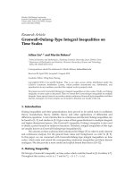
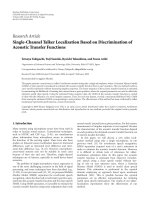
Figure 1: Convolutional face finder pipeline.
The remainder of this paper is organized as follows: an
overview of the convolutional face finder technique is given
in Section 2. Section 3 presents the methodology used for
embedding such an algorithm. Section 4 details this method-
ology on the CFF case study. Experimental results for DSP-
and RISC-based platforms are provided in Section 4. Finally,

conclusions and perspectives are drawn in Section 5.
2. CFF ALGORITHM OVERVIEW
The convolutional face finder was presented in [8]andrelies
on convolutional neural networks (CNN) introduced and
successfully used by LeCun et al. [14]. It consists of a pipeline
of convolutions and subsampling operations (see Figure 1).
This pipeline performs automatic feature extraction in image
areas of size 32
× 36, and classification of the extracted fea-
tures, in a single integrated scheme.
The convolutional neural network, shown in Figure 1,
consists of a set of three different kinds of layers. Layers C
i
are called convolutional layers, which contain a certain num-
ber of planes. Layer C
1
is connected to the retina, receiving
the image area to classify as face or non-face. Each unit in
a plane receives input from a small neighbourhood (biolog-
ical local receptive field) in the planes of the previous layer.
Each plane can be considered as a feature map that has a fixed
feature detector corresponding to a pure convolution with a
trainable mask, applied over the planes in the previous layer.
A trainable bias is added to the results of each convolutional
mask. Multiple planes are used in each layer so that multiple
features can be detected.
Once a feature has been detected, its exact location is less
important. Hence, each convolutional layer C
i
is typically fol-

lowed by another layer S
i
that performs local averaging and
subsampling operations. More precisely, each layer S
i
out-
put data is the result of the average of four input data in C
i
,
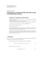
Conv olution 5 × 5 Subsampling
Figure 2: Receptive fields for convolution and subsampling for a
feature map of layers C
1
-S
1
.
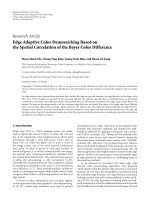
Coarse
detection
Fine
detection
Figure 3: Face detection block diagram.
(see Figure 2) multiplied by a trainable coefficient, added to a
trainable bias, and passed through a hyperbolic tangent func-
tion, used as an activation function. This subsampling op-
eration reduces the dimensionality of the input by two and
increases the degrees of invariance to translation, scale, and
deformation of the learnt patterns.
In CFF, la yers C
1
and C

2
perform convolutions with
trainable masks of dimensions 5
× 5and3× 3, respec-
tively. Layer C
1
contains four feature maps and therefore per-
forms four convolutions on the input image. Layers S
1
and C
2
are partially connected. Mixing the outputs of feature maps
helps in combining different features, thus in extracting more
complex information. Layer C
2
has 14 feature maps. Each of
the four subsampled feature maps of S
1
is convolved by two
different trainable masks 3
× 3, providing eight feature maps
in C
2
. The other six feature maps of C
2
are obtained by fus-
ing the results of two convolutions on each possible pair of
S
1
feature maps.

Layers N
1
and N
2
contain simple sigmoid neurons. The
role of these layers is to perform classification after feature ex-
traction and input dimensionality reduction are performed.
In layer N
1
, each neuron is fully connected to exactly one fea-
turemapoflayerS
2
. The unique neuron of layer N
2
is fully
connected to all the neurons of layer N
1
. The output of this
neuron is used to classify the input image as face (positive
answer) or nonface (negative answer). All parameters (con-
volution kernels, subsampling coefficients, biases) have been
learnt automatically using a modified version of the back-
propagation algorithm with momentum, from a large train-
ing set of faces [8].
As depicted in Figure 3, the process of face detection with
CFF is performed in two steps. The first one can be consid-
ered as a coarse detection and returns positive responses to
gather face candidate positions. The second one called fine
detection performs a refined search in an area around each
face candidate found in the first step.

Franck Mamalet et al. 3
In [8], the authors present both the training methodol-
ogy to learn the coefficients, and the face localization process
when training is completed. In this paper, we will focus on
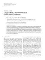
the face localization process. Figure 4 presents in detail the
steps of this face localization process.
(i) Coarse detection is processed as follows: CFF is ap-
plied on a pyramid of scaled versions of the original
image (see Figure 4-1) in order to handle faces of dif-
ferent sizes: each scale produces a map of face candi-
dates (see Figure 4-2) which is fused back to the in-
put image resolution and produces clusters of positive
answers (see Figure 4-3). For each cluster, a represen-
tative face is computed as the centroid of its candidate
face centers and sizes, weighted by their individual net-
work responses.
(ii) Fine detection takes those candidates as input and lo-
cally applies CFF on a small pyramid around the face
candidate center position (see Figure 4-4). The volume
of positive answers is considered in order to take the
classification decision, that is, face or non-face (see
Figure 4-5). Finally, overlapping candidates are fused
to suppress multidetection of the same face.
The acronym CFF will be used either for the detection
pipeline or for the entire algorithm.
3. PORTING CFF TO EMBEDDED PLATFORMS:
MAIN ISSUES AND METHODOLOGY
In order to implement complex algorithms on an embedded
target processor, compilers are the tools used to optimize the
instructions flow. In the last decade, many research activ-

ities have been carried out on instructions flow optimiza-
tions [15] and optimizing compilers [16], and some have
led to industrial products such as the Metrowerks compiler
for SC140 [17, 18]. However, compilers can only cope with
the inst ructions flow optimization and parallelization. Even
if these compilers mostly avoid human assembly program-
ming, they only deal with local optimizations and many op-
timizations still need to be carried out by high-le vel code
rewriting .
Other tools enable us to deal with these high level op-
timizations. First of all, high level profiling tools such as
VTune software [19] are dedicated to pointing out the most
consuming parts of the code using on-target time-sampling
simulations. Also, memory accesses analysis tools [20]can
be used to identify memory access bottlenecks. Some recent
works try to propose semiautomatic tools for data transfer
and storage optimizations [21]. This work relies on the fol-
lowing methodology which is only driven by high-level code
profiling; further investigation will be carried out to auto-
mate our optimization process.
Our approach is based on iterations of high-level code
optimizations and profiling to focus firstly on the most con-
suming functions of CPU resources. When dealing with an
algorithm such as CFF, the first step towards embedded im-
plementation is to avoid floating-point calculation. This step
is called data optimization in [22] and is achieved thanks
12
3
4
5

CFF
CFF
CFF
CFF
Figure 4: The different steps of the process of face localization.
Processor
architecture/
instruction set
Floating-point
code
Fixed-point
code
Data
dynamics
analysis
Algorithm
optimization
Code
optimization
Memory
optimization
Profiling
Timing
constraint
Memory
constraint
Figure 5: Diagram of followed methodology.
to a fractional transformation in accordance with data dy-
namics and processors data path. This also requires a strong
verification of the accuracy of these transformations which

can otherwise lead to incorrect results. The next steps of the
methodology are iterations of a tri-optimization flow (code,
memory, and algorithm) controlled by an on-target profiling
(see Figure 5).
Profiling tools depend on the target platfor m: for in-
stance, we use the VTune software [19] on an Xscale-based
platform to profile the compiled code directly on target, and
global timing information to evaluate the speed-up fac tor af-
ter each optimization iteration.
4 EURASIP Journal on Embedded Systems
Table 1: Results of CFF on different test sets for the floating- and fixed-point versions.
Faces size 36 to 300 pixels high 18 to 300
Threshold 10 17 17
Detection rate (%) False alarms Detection rate (%) False alarms Detectionrate(%) Falsealarms
Floating-
point
version
CMU 84,89 6 80,12 0 87,99 2
CINEMA
∗
87,32 8 82,97 1 82,97 4
WEB
∗
87,98 2 83,97 0 91,98 2
ATT 97,25 0 96,50 0 96,75 0
Total 89,20 22 85,71 1 90,47 8
Fixed-
point
version
CMU 86,75 4 81,37 0 88,20 3

CINEMA
∗
88,41 6 82,25 3 85,14 9
WEB
∗
88,98 1 86,17 1 92,38 5
ATT 99,25 0 97,50 0 96,50 0
Total 90,71 15 86,85 4 90,95 17
∗
CINEMA and WEB are test sets of, respectively, 276 and 499 faces kindly provided by GarciaandDelakis [8].
We will illustrate our methodology on the CFF imple-
mentation, whose starting point was a floating point arith-
metic version and required a memory allocation of 3.8 M-
Bytes to process a QCIF format image (176
×144 pixels). The
reference complexity analysis of the floating-point version of
the CFF shows that it requires 3 seconds to compute a sin-
gle QCIF image on a 624 MHz Xscale processor. Hereafter,
we present in detail each step of this methodology and the
achieved performance results.
4. OPTIMIZING THE CFF ALGORITHM
4.1. Fractional transformation
CFF reference software was entirely written using floating-
point arithmetic. Mobile-embedded target platforms lack
floating-point hardware accelerator for power consump-
tion reasons. Floating-point computations are usually im-
plemented by software, but these are high CPU consuming
functions. The first step towards embedding the algorithm
is to transform the floating-point computations into frac-
tional ones. Since one of our target platforms was the 16 bit

DSP Starcore SC140, fractional Q15 arithmetic [23]wasre-
quired (Q31 arithmetic may be used when more precision is
needed).
The main advantage of the CFF algorithm is that the re-
sults of the subsampling layers S
1
and S
2
pass through hy-
perbolic tangent functions (which limits the data dynam-
ics), thus reducing the risk for common issues of fixed-point
computations such as arithmetic dynamic expansion and
saturation. A simple methodology was used to normalize
and transform each neural network coefficient in fixed-point
arithmetic and compare the results with the floating-point
version. Each coefficients kernel for each layer is first nor-
malizedtopreventaccumulationoverflow(sumofabsolute
values strictly lower than one). Each coefficient is then fitted
to 16 bits fractional representation. Precision tests are carried
out experimentally on standard face databases.
The main constraint of this transformation was to main-
tain the efficiency of the face detector. The benchmarking was
done on different test sets of images, including the CMU test
set (the most widely used data set in the literature). Ta ble 1
gives the detection rates of the floating- and fixed-point ver-
sions on four test sets for different CFF configurations (vary-
ing output volume threshold and minimum allowed face
size).
The comparison of the floating-point and fixed-point
versions shows no significant loss in efficiency and detection

rates are equivalent to the ones previously published in [8].
They are even better on some parts of the selected test sets.
What is especially noticeable about the CFF efficiency is the
very low level of false alarms, even after the fractional trans-
formation.
4.2. Memory optimization
Due to the computational redundancy in the CFF algorithm,
the reference software was processing layer by layer on the
whole image (and scaled versions of the original image). This
configuration is not suitable for an embedded platform since
even for small QCIF images, 3.8 MBytes were allocated (e.g.,
the targeted SC140 DSP platform embeds only 512 kB of
SRam).
In order to reduce this memory allocation without in-
creasing the required amount of computations, a study
was carried out on the data dependency in the algorithm.
Figure 6(a) shows the amount of data needed in each layer
in order to compute a single output of each neuron in layer
N
1
. This figure is similar to Figure 1 restricted to one feature
map by layer.
Figure 6(b) illustrates the differential computation be-
tween two neighbouring outputs (south side) of neuron layer
N
1
. Slashed (resp., unslashed) grey parts are unused (resp.,
reused) previously computed data, whereas dark rectangles
are newly computed data.
Franck Mamalet et al. 5

6
7
12
14
16
14
28
32
36
32
Layer N
1
:
convolve
6 × 7
Layer S
2
:
subsample
Layer C
2
:
convolve
3 × 3
Layer S
1
:
subsample
Layer C
1

:
convolve
5 × 5
(a)
67
12
2
4
14
28
4
8
32
N
1
S
2
C
2
S
1
C
1
(b)
Figure 6: CFF data flow. (a) Amount of data needed in each layer,
(b) differential computation between two neighbouring outputs
(south side).
Since Figure 6(b) shows that intermediate computation
from previous lines has to be kept as input of layers C
2

and
N
1
, the maximum gain in terms of memory footprint is
achieved for a line-by-line processing of the output of layer
N
1
. Thus, in the final implementation, in order to compute
one output line of layer N
1
, we use 7 input lines of this layer.
These input lines can be computed line by line in layer S
2
using two o utput lines of layer C
2
. These two output lines re-
quire four input lines for layer C
2
. Two of these four output
lines are common with the previously computed lines, and
the two others require four output lines of layer C
1
. These
four output lines of layer C
1
are computed using eight lines
of the input image.
Tab le 2 represents the memory allocation analysis for the
full image processing and the line-by-line processing. Each
stage of output memory is parameterized by W and H, the

width and height of the input image.
For a QCIF image, the gain in memory footprint is about
21. Other memory allocation optimizations (e.g., on-scaled
images computation) have been made on the reference soft-
ware leading to a memory footprint of 220 kB compared to
the 3.8 Mbytes of the original version.
4.3. Code optimization: parallelism exploitation
One of our target-embedded platforms is a Starcore SC140
DSP which has 4 ALUs and multiplier capabilities. This pro-
cessor is able to load eight 16 bits words and to compute
4 multiplication-accumulations (MACs) in one cycle. The
main limitation to taking advantage of this parallelism is
that the data’s alignment constraints need to be satisfied: the
Move.4F instruction [24] which loads four 16 bits-word data
Table 2: Memory allocation for full image and line-by-line process-
ing.
Layer
Number of Full image Line-by-line
branches processing processing
C
1
output 4 (W − 4)
∗
(H − 4) (W − 4)
∗
4
S
1
Output 4 (W − 4)/2
∗

(H − 4)/2 (W − 4)/2
∗
4
C
2
Output 14 (W − 8)/2
∗
(H − 8)/2 (W − 8)/2
∗
2
S
2
Output 14 (W − 8)/4
∗
(H − 8)/4 (W − 8)/4
∗
7
N
1
Output 14 (W − 28)/4
∗
(H − 32)/4 (W − 28)/4
∗
1
Total — 10.25
∗
W
∗
H + ··· 66
∗

W + ···
is only allowed for an eight-bytes aligned pointer and can
be generated automatically by the compiler by appropriate
C code rewriting and alignment directive use.
Let us analyze the first layer (C
1
) which the profiling tool
points out as being the most complex step of the CFF al-
gorithm: each of the four feature maps of this layer con-
sists of a convolution by a 5
× 5 kernel. Without any par-
allelization one convolution requires 25 data loads, 25 coef-
ficient loads, 25 MACs instructions, and one store instruc-
tion. Since the Starcore is able to compute four MACs in one
cycle, the theoretical minimum cycle count for processing
25 MACs (without load and store count) is [25/4]
= 7cy-
cles. Without aligned load instructions, the Starcore is able
to process two 16 bits load instructions by cycle (in parallel
with the MACs instructions). Thus, due to the number of
load and store instructions, one convolution would require
at least [(25 + 25 + 1)/2]
= 26 cycles. The main goal in or-
der to optimize such a function is to reduce the number of
load and store instructions by using the Move.4F instruc-
tion.
Input data and coefficients are 16 bits words. Assuming
that the first element is 8 bytes aligned, the Starcore should
be able to load 4 data and/or coefficients in a single cycle.
But, the 5

× 5 convolution processing is done on any image
of the pyramid w hose width is not necessarily multiple of 4.
Thus if the first top-left pixel in the image is 8 bytes aligned,
the first pixel on the second line will probably not be aligned
preventing any use of multiple load instruction on these data.
On the other hand, using aligned loads on coefficients would
imply dividing the 5
× 5 kernel matrix into several matrices
4
× 4, 1 × 4, and 5 × 1, making the convolution processing
more complex.
In order to reduce the number of load instructions per
convolution, the proposed solution consists of factorizing the
coefficients loads in order to process the 5
× 5 convolution
several times (multisample processing).
Figure 7 presents the factorization process. Convolutions
are done by 25 iterations on the whole block of pixels. At
each iteration, groups of four multiplication-accumulations
with a single coefficient are performed. This requires a
temporal store and load of intermediate processing (e.g.,
c[0, 0]
· x[0, 0], ), but, since this intermediate matrix can
be 8 bytes aligned, four intermediate computations can be
loaded or saved in a single instruction. Ta ble 3 sums up
the amount of load and store instructions needed for the
6 EURASIP Journal on Embedded Systems
y
0
0

= c
0
0
· x
0
0
+ c
1
0
· x
1
0
+ ···+ c
3
4
· x
3
4
+ c
4
4
· x
4
4
y
1
0
= c
0
0

· x
1
0
+ c
1
0
· x
2
0
+ ···+ c
3
4
· x
4
4
+ c
4
4
· x
5
4
y
2
0
= c
0
0
· x
2
0

+ c
1
0
· x
3
0
+ ···+ c
3
4
· x
5
4
+ c
4
4
· x
6
4
y
3
0
= c
0
0
· x
3
0
+ c
1
0

· x
4
0
+ ···+ c
3
4
· x
6
4
+ c
4
4
· x
7
4
.
.
.
Group 0
y
i
j
= c
0
0
· x
i
j
+ c
1

0
· x
i+1
j
+ ···+ c
3
4
· x
i+3
j+4
+ c
4
4
· x
i+4
j+4
.
.
.
y
W−5
H
−5
= c
0
0
· x
W−5
H
−5

+ c
1
0
· x
W−4
H
−5
+ ···+ c
3
4
· x
W−2
H
−1
+ c
4
4
· x
W−1
H
−1
Group N
Iter. 0 Iter. 0 Iter . 23 Iter. 24
Figure 7: Parallelism exploitation: parallelization process.
Table 3: Load and store count for the 5
× 5 convolution of a block
of size S
= (W − 4)
∗
(H − 4).

Initial version Modified version
Nb load coef. instructions 25
∗
S 25
Nb load data instructions
25
∗
S 25
∗
S
Nb load/store instructions for
0 25
∗
S/4+25
∗
S/4
intermediate results
Final store instructions S 0
Total 51
∗
S 25 + 37.5
∗
S
5 × 5 convolution of an image of size W
∗
H in function of
S
= (W − 4)
∗
(H − 4), the number of convolutions.

When processing four output lines of layer C
1
as depicted
in the previous paragraph, the gain in terms of load/store
instructions is for a QCIF image (W
= 176, H = 8):
51
∗
S − 25 − 37.5
∗
S
51
∗
S
=
27
102
−
25
51
∗
4
∗
(W − 4)
= 26, 4%.
(1)
We achieve the same gain in terms of the number of cycles
by convolution with this factorized version (the inner loop
takes 3 cycles to compute 4 MACs, compared to the 4 cycles
required by the original version).

This optimization may also be applied on processors us-
ing SIMD instructions such as WMMX instructions on an
Xscale-embedded processor. The efficiency of this optimiza-
tion on these processors has not yet been evaluated.
4.4. Algorithm optimization
In this section, we present two examples of algorithmic op-
timization applied on the CFF which lead to a great increase
in performance.
N
N +1
2

p
k,l
p
i,j
C
(N+1)×(N+1)
4
∗
C
N×N
p

m,n
S
Figure 8: Convolution and subsampling fusion process.
Table 4: Instruction counts for sequential and fused versions.
Number of Mac instructions
C

N×N
+ S 4
∗
N2+4
C
(N+1)×(N+1)
(N +1)
2
Gain (3
∗
N
2
− 2
∗
N +3)/(4
∗
N
2
+4)
Gain (N
= 5) 65%
Gain (N
= 3) 60%
4.4.1. Convolution and subsampling fusion
When considering the data dependency (see Figure 6), we
can see that, at each subsampling layer, there is no overlap-
ping between input data to produce two neighbor subsam-
pled elements.
The output element value p
i, j

(cf. Figure 8)ofaC
i
-S
i
(i =
{
1, 2}) couple can be expressed as follows:
p
i, j
= α
∗

p

2i,2 j
+ p

2i,2 j+1
+ p

2i+1,2 j
+ p

2i+1,2 j+1

,
p

m,n
=

N

k=0
N

l=0
c
k,l
∗

p
m+k,n+l
,
p
i, j
= α
∗

N

k=0
N

l=0
c
k,l
∗

p
2i+k,2 j+l

+ ···
+
N

k=0
N

l=0
c
k,l
∗

p
2i+1+k,2 j+1+l

=
N+1

k=0
N+1

l=0
c
k,l
∗

p
k,l
,
(2)

where N is the convolution size, α is the subsampling coeffi-
cient, c
k,l
are the convolution coefficients, p

i, j
are the inputs
of the subsampling,

p
k,l
are the inputs of the convolution, c
k,l
are the weighted sums of one-to-four c
k,l
coefficients.
So, we propose fusing each N by N convolution (C
N×N
)
followed by subsampling (S) into a (N +1)by(N +1)con-
volution (C
(N+1)×(N+1)
) (see Figure 8).
Tab le 4 gives the computational and memory access com-
plexities for each version. The gain achieved by this algorith-
mic optimization is huge in terms of the computational cost,
65% (resp., 60%) is obtained for the first layer C
1
-S
1

(resp.,
second layer C
2
-S
2
) of the CFF.
Franck Mamalet et al. 7
Coarse
detection
Fine
detection
n
n +1
> Th.
?
Figure 9: Functional diagram of the CFF video.
Furthermore, the merging of convolution and sub-
sampling coefficients avoids multiple fractional arithmetic
rounding, enabling slight improvements of benchmark re-
sults (e.g., on CMU test set +0, 2% on face detection r ate and
2 false alarms versus 4).
4.4.2. Tracking adaptation
The CFF algorithm was first dedicated to still-image index-
ing, and thus, the process considers only an input image. One
of our aims was to adapt this algorithm to video indexing.
Since the algorithm was organized in two stages; one
coarse detection on the whole image and a second one in a
finer pyramid centered at each candidate’s face location, we
have used this second stage for tracking the detected faces in
successive frames.

The proposed video-based CFF algorithm can be seen as
an intra and inter processing of images by analogy with im-
age coding (H26x or Mpeg, [25]). One image among N is
computed by the coarse detection (intra detection), and we
do only apply the fine detection on the following images at
each candidates’ face location given by the prev ious image
(inter detection). Fine detection using a local pyramid en-
ables us to cope with the face size variation (zoom), and the
window search area being 20 pixels around the previous face
center enables us to handle most face motion issues.
In order to avoid the false detection alarms on “In-
tra” images, an adaptive volume threshold has been intro-
duced downstream to the coarse detection. This threshold is
adapted using an infinite impulse response filter whenever an
Intra detection and its fol lowing Inter detection have contra-
dictory answers. Figure 9 gives a functional description of the
video adaptation.
Since profiling on coarse and fine detect ion was balanced
(54% for coarse detection and 46% for fine detection under
a Vtune profiling on Xscale PXA27x processor), we may at
least foresee a speed-up factor of two. But, simulations and
profiling on several platforms point out that this video-based
CFF is about 3 times faster than the image-based one (for
N
= 6). This is mainly due to false detections of the coarse
detection being removed by the first iteration of the fine de-
tection, and so no longer tracked on the following images.
4.5. Performance results
Tab le 5 summar izes the speed-up factor obtained on a QCIF
video test sequence (120 first frames of the Mpeg Foreman

Table 5: CFF and CFF video processing speed.
Xscale
PXA27x @
624 MHz
Starcore
SC140 @
275 MHz
Pentium IV
@3.2GHz
Floating-point
0.3 fr/s — 10 fr/s
reference
Fixed-point
4.5 fr/s 7fr/s 32 fr/s
version
Code
— 9fr/s —
optimization
Algorithm
6.5 fr/s 13 fr/s 58 fr/s
optimization (4.4.1)
Tracking
16.5 fr/s 35 fr/s 180 fr/s
adaptation (4.4.2)
sequence) for each kind of optimizations done on the face
detector.
A speed-up factor of 55 is obtained between the orig-
inal floating-point version and the fixed-point face tracker
on the Xscale platform enabling face-tracking-based services
on mobile terminals. Without tracking adaptation, the im-

provement is still huge (22 times). Real-time face detection
is also achieved on highly parallel DSP architecture. Tabl e 5
also points out the strong impact of algorithm optimization
on the application performance. Optimizations carried out
for embedded platforms are also useful on a PC target a ble to
process real time TV format video streams.
As a comparison with other embedded robust face de-
tection implementations, we consider the works presented
in [9, 11] that both propose AdaBoost-optimized solutions
(based on the Viola and Jones approach [10]), respectively,
on an ARM926 processor and a TI TMS320C6205. The Vi-
ola and Jones method is known to be less efficient than CFF
[8], with a good detection rate of 76.1% w ith 10 false alarms
for the CMU test set. The number of frames per second
achieved by these implementations is, respectively, about 4
and 3 Hz for QVGA-like video format which is comparable
to our frame-by-frame implementation of the CFF process-
ing. However, the tracking adaptation enables us to 3 times
outperform these frame rates.
Furthermore, as depicted before, the memory footprint
has been reduced from 3.8 MBytes to 220 kBytes by the mem-
ory optimization step.
5. CONCLUSION AND PERSPECTIVES
In this paper, we have presented the implementation of a
state-of-the-art face detector on two kinds of programmable
embedded platforms. We have shown that both high de-
tection rates and fast processing are achieved by apply-
ing our optimization flow methodology. Memory and code
restructuring in conjunction with algorithm adaptation
lead to significant improvement. This study proves that

CNN algorithms are well suited for embedded implementa-
tion since they stand up to fractional transformations and
they offer good opportunities for memory and algorithm
8 EURASIP Journal on Embedded Systems
optimizations. Indeed, we obtain a speed-up factor of 55 on
an Xscale-PXA27x-based platform and real-time video pro-
cessing(upto35QCIFfr/s)onaStarcoreDSP.Higheffi-
ciency is maintained, with a detection rate of 87% on the
CMU test set and only 4 false alarms.
One of our final objectives is to provide an embedded
face recognition system for biometrics applications. Usually,
face-based identification systems require precise face and fa-
cial feature localization and also fine facial feature position-
ing. The first step depicted in this paper was the real-time im-
plementation of this face detector by software optimizations.
The second step is to precisely locate facial features, and we
are now working on the implementation of a facial feature
detector based on the same principles which is called C3F for
convolutional face feature finder [26].
Furthermore, this study points out that the pipeline of
convolutional and subsampling filters denotes high intrin-
sic and hidden parallelisms which will be exploited in future
works with dedicated hardware implementation of CFF and
C3F.
REFERENCES
[1]M H.Yang,D.J.Kriegman,andN.Ahuja,“Detectingfaces
in images: a survey,” IEEE Transactions on Pattern Analysis and
Machine Intelligence, vol. 24, no. 1, pp. 34–58, 2002.
[2] K. C. Yow and R. Cipolla, “Feature-based human face detec-
tion,” Image and Vision Computing, vol. 15, no. 9, pp. 713–735,

1997.
[3] C C. Lin and W C. Lin, “Extracting facial features by an in-
hibitory mechanism based on gradient distributions,” Pattern
Recognition, vol. 29, no. 12, pp. 2079–2101, 1996.
[4] I. Craw, D. Tock, and A. Bennett, “Finding face features,” in
Proceedings of the 2nd European Conference on Computer Vision
(ECCV ’92), pp. 92–96, Santa Margherita Ligure, Italy, May
1992.
[5] A. Lanitis, C. J. Taylor, and T. F. Cootes, “Automatic face iden-
tification system using flexible appearance models,” Image and
Vision Computing, vol. 13, no. 5, pp. 393–401, 1995.
[6] B. Moghaddam and A. Pentland, “Probabilistic visual learning
for object representation,” IEEE Transactions on Pattern Anal-
ysis and Machine Intelligence, vol. 19, no. 7, pp. 696–710, 1997.
[7] K K. Sung and T. Poggio, “Example-based learning for view-
based human face detection,” IEEE Transactions on Pattern
Analysis and Machine Intelligence, vol. 20, no. 1, pp. 39–51,
1998.
[8] C. Garcia and M. Delakis, “Convolutional face finder: a neural
architecture for fast and robust face detection,” IEEE Trans-
actions on Pattern Analysis and Machine Intelligence, vol. 26,
no. 11, pp. 1408–1423, 2004.
[9] X. Tang, Z. Ou, T. Su, and P. Zhao, “Cascade AdaBoost clas-
sifiers with stage features optimization for cellular phone em-
bedded face detection system,” in Proceedings of the 1st Inter-
national Conference on Natural Computation (ICNC ’05),pp.
688–697, Changsha, China, August 2005.
[10] P. Viola and M. Jones, “Rapid object detection using a boosted
cascade of simple features,” in Proceedings of the IEEE Com-
puter Society Conference on Computer Vision and Pattern

Recognition, vol. 1, pp. 511–518, Kauai, Hawaii, USA, Decem-
ber 2001.
[11] J B. Kim, Y. H. Sung, and S C. Kee, “A fast and robust face
detection based on module switching network,” in Proceedings
of the 6th IEEE International Conference on Automatic Face and
Gesture Recognition (FGR ’04) , pp. 409–414, Seoul, Korea, May
2004.
[12] T. Theocharides, G. Link, N. Vijaykrishnan, M. J. Irwin, and
W. Wolf, “Embedded hardware face detection,” in Proceedings
of the 17th IEEE International Conference on VLSI Design,pp.
133–138, Mumbai, India, January 2004.
[13] H. A. Rowley, S. Baluja, and T. Kanade, “Neural network-
based face detection,” IEEE Transactions on Pattern Analysis
and Machine Intelligence, vol. 20, no. 1, pp. 23–38, 1998.
[14] Y. LeCun, L. Bottou, Y. Beng io, and P. Haffner, “Gradient-
based learning applied to document recognition,” Proceedings
of the IEEE, vol. 86, no. 11, pp. 2278–2324, 1998.
[15] V. Tiwari, S. Malik, and A. Wolfe, “Compilation techniques for
low energy: an overview,” in Proceedings of IEEE Symposium
on Low Power Electronics, pp. 38–39, San Diego, Calif, USA,
October 1994.
[16] S. Muchnick, Advanced Compiler Design & Implementation,
Morgan Kaufmann, San Francisco, Calif, USA, 1997.
[17] J. C. Bauer, E. Closse, E. Flamand, M. Poize, J. Pulou, and P.
Penier, “SAXO: a retargetable optimized compiler for DSPs,”
in Proceedings of the 8th International Conference on Signal
Processing Applications & Technology (ICSPAT ’97),SanDiego,
Calif, USA, September 1997.
[18] V. Palanciuc, D. Badea, C. Ilas, and E. Flamand, “A spill code
reduction technique for EPIC architectures,” in Proceedings of

the 1st Workshop on Explicitly Parallel Instruction Computing
Architectures and Compiler Technology (EPIC-1 ’01)
, Austin,
Tex, USA, September 2001.
[19] INTEL PCA Optimization guide, el.
com/pcadn/.
[20] T. Van Achteren, G. Deconinck, F. Catthoor, and R. Lauwere-
ins, “Data reuse exploration techniques for loop-dominated
applications,” in Proceedings of Design, Automation and Test
in Europe Conference and Exhibition (DATE ’02), pp. 428–435,
Paris, France, March 2002.
[21] F. Catthoor, K. Danckaert, C. Kulkarni, et al., Data Access and
Storage Management for Embedded Programmable Processors,
Kluwer Academic, Boston, Mass, USA, 2002.
[22] T. Simunic, L. Benini, G. De Micheli, and M. Hans, “Source
code optimization and profiling of energy consumption in
embedded systems,” in Proceedings of the 13th International
Symposium on System Synthesis (ISSS ’00), pp. 193–198,
Madrid, Spain, September 2000.
[23] A. Bateman and I. Paterson-Stephens, The DSP Handbook, Al-
gorithms, Applications and Design Techniques, Prentice-Hall,
Upper Saddle River, NJ, USA, 2002.
[24] “SC140 DSP Core Reference Manual Second Revision,” Mo-
torola Corporation, 2001.
[25] MPEG-4 visual version 1, “Coding of audio-visual objects—
Part 2: visual,” ISO/IEC JTC1 14 496-2, 1999.
[26] S. Duffner and C. Garcia, “A connexionist approach for ro-
bust and precise facial feature detection in complex scenes,” in
Proceedings of the 4th International Symposium on Image and
Signal Processing and Analysis (ISPA ’05), pp. 316–321, Zagreb,

Croatia, September 2005.