Báo cáo hóa học: " Research Article Analysis of Transient and Steady-State Behavior of a Multichannel Filtered-x Partial-Error Affine Projection Algorithm" docx
Bạn đang xem bản rút gọn của tài liệu. Xem và tải ngay bản đầy đủ của tài liệu tại đây (1.39 MB, 15 trang )
Hindawi Publishing Corporation
EURASIP Journal on Audio, Speech, and Music Processing
Volume 2007, Article ID 31314, 15 pages
doi:10.1155/2007/31314
Research Article
Analysis of Transient and Steady-State Behavior
of a Multichannel Filtered-x Partial-Error Affine
Projection Algorithm
Alberto Carini
1
and Giovanni L. Sicuranza
2
1
Information Science and Technology Institute, University of Urbino “Carlo Bo”, 61029 Urbino, Italy
2
Department of Electrical, Electronic and Computer Engineering, University of Trieste, 34127 Trieste, Italy
Received 28 April 2006; Revised 24 November 2006; Accepted 27 November 2006
Recommended by Kutluyil Dogancay
The paper provides an analysis of the transient and the steady-state behavior of a filtered-x par tial-error affine projection algo-
rithm suitable for multichannel active noise control. The analysis relies on energy conserv ation arguments, it does not apply the
independence theory nor does it impose any restriction to the signal distributions. The paper shows that the partial-error filtered-x
affine projection algorithm in presence of stationary input signals converges to a cyclostationar y process, that is, the mean value of
the coefficient vector, the mean-square error and the mean-square deviation tend to periodic functions of the sample time.
Copyright © 2007 A. Carini and G. L. Sicuranza. This is an open access article distributed under the Creative Commons
Attribution License, which permits unrestricted use, distribution, and reproduction in any medium, provided the original work is
properly cited.
1. INTRODUCTION
Active noise controllers are based on the destructive inter-
ference in given locations of the noise produced by some
primary sources and the interfering signals generated by
some secondary sources driven by an adaptive controller [1].
A commonly used strategy is based on the so-called feed-
forward methods, where some reference signals measured in
the proximity of the noise source are available. These signals
are used together with the error signals captured in the prox-
imity of the zone to be silenced in order to a dapt the con-
troller. Single-channel and multichannel schemes have been
proposed in the literature according to the number of ref-
erence sensors, error sensors, and secondary sources used.
A single-channel active noise controller makes u se of a sin-
gle reference sensor, actuator, and error sensor and it gives,
in principle, attenuation of the undesired disturbance in the
proximity of the point where the error sensor is located. In
the multichannel approach, in order to spatially extend the
silenced region, multiple reference sensors, actuators and er-
ror sensors are used. Due to the multiplicity of the signals in-
volved, to the strong correlations between them and to the
long impulse response of the acoustic paths, multichannel
active noise controllers suffer the complexity of the coeffi-
cient updates, the data storage requirements, and the slow
convergence of the adaptive algorithms [2]. To improve the
convergence speed, different filtered-x affine projection (FX-
AP) algorithms have been used [3, 4] in place of the usual
filtered-x LMS algorithms, but at the expense of a further,
even though limited, increment of the complexity of updates.
Various techniques have been proposed in the literature to
keep low the implementation complexity of adaptive FIR fil-
ters having long impulse responses. Most of them can be use-
fully applied to the filtered-x algor ithms, too, especially in
the multichannel situations. A first approach is based on the
so-called interpolated FIR filters [5], where a few impulse re-
sponse samples are removed and then their values are derived
using some type of interpolation scheme. However, the suc-
cess of this implementation is based on the hypothesis that
practical FIR filters have an impulse response with a smooth
predictable envelope, which is not applicable to the acous-
tic paths. Another approach is based on data-selective up-
dates which are sparse in time. This approach can be suit-
ably described in the framework of the set-membership fil-
tering (SMF) where a filter is designed to achieve a specified
bound on the magnitude of the output error [6]. Finally, a
set of well-established techniques is based on selective partial
updates (PU) where selected blocks of filter coefficients are
updated at every iteration in a sequential or periodic manner
[7] or by using an appropriate selection criterion [8]. Among
2 EURASIP Journal on Audio, Speech, and Music Processing
the partial update str ategies, a simple yet effective approach
is provided by the partial error (PE) technique, which has
been first applied in [7] for reducing the complexity of linear
multichannel controllers equipped with the filtered-x LMS
algorithm. The PE technique consists in using sequentially at
each iteration only one of the K error sensor signals in place
of their combination and it is capable to reduce the adap-
tation complexity with a factor K.In[9], the PE technique
was applied, together with other methods, for reducing the
computational load of multichannel active noise controllers
equipped with filtered-x affine projection (AP) algorithms.
When dealing with novel adaptive filters, it is important to
assess their performance not only through extensive simu-
lations but also with theoretical analysis results. In the lit-
erature, very few results deal with the analysis of filtered-x,
affine projection or partial-update algorithms. The conver-
gence analysis results for these algorithms are often based on
the independence theory (IT) and they constrain the proba-
bility distribution of the input signal to be Gaussian or spher-
ically invariant [10]. The IT hypothesis assumes statistical
independence of time-lagged input data vectors. As it is too
strong for filtered-x LMS [11] and AP algorithms [12], dif-
ferent approaches have been studied in the literature in order
to overcome this hypothesis. In [11], an analysis of the mean
weight behavior of the filtered-x LMS algorithm, based only
on neglecting the correlation between coefficient and signal
vectors, is presented. Moreover, the analysis of [11]doesnot
impose any restriction on the signal distributions. Another
analysis approach that avoids IT is applied in [12] for the
mean-square performance analysis of AP algorithms. This
relies on energy conservation arguments, and no restriction
is imposed on the signal distributions. In [4], we applied and
adapted the approach of [12] for analyzing the convergence
behavior of multichannel FX-AP algorithms. In this paper,
we extend the analysis approach of [4] and study the tran-
sient and steady-state behavior of a filtered-x partial error
affine projection (FX-PE-AP) algorithm. The paper shows
that the FX-PE-AP algorithm in presence of stationary input
signals converges to a cyclostationary process, that is, that the
mean value of the coefficient vector, the mean-square-error,
and the mean-square-deviation tend to periodic functions of
the sample time. We also show the FX-PE-AP algorithm is
capable to reduce the adaptation complexity with a factor K
with respect to an approximate FX-AP algorithm introduced
in [4], but it also reduces the convergence speed by the same
factor.
The paper is orga nized as follows. Section 2 reviews
the multichannel feedforward active noise controller struc-
ture and introduces the FX-PE-AP algorithm. Section 3
discusses the asymptotic solution of the FX-PE-AP algo-
rithm and compares it with that of FX-AP algorithms and
with the minimum-mean-square solution of the ANC prob-
lem. Section 4 presents the analysis of the transient and
steady-state behavior of the FX-PE-AP algorithm. Section 5
provides some experimental results. Conclusions follow in
Section 6.
Throughout this paper, small boldface letters are used to
denote vectors and bold capital letters are used to denote ma-
trices, for example, x and X, all vectors are column vectors,
the boldface symbol I
indicates an identity matrix of appro-
priate dimensions, the symbol
denotes linear convolution,
diag
{···}is a block-diagonal matrix of the entries, E[·]de-
notes mathematical expectation,
·
2
Σ
is the weighted Eu-
clidean norm, for example,
w
2
Σ
= w
T
Σw with Σ a symmet-
ric positive definite matr ix, vec
{·} indicates the vector oper-
ator and vec
−1
{·} the inverse vector operator that returns a
square matrix from an input vector of appropriate dimen-
sions,
⊗ denotes the Kronecker product, a%b is the remain-
der of the division of a by b,and
|a| is the absolute value
of a.
2. THE PARTIAL-ERROR FILTERED-x AP ALGORITHM
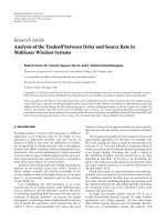
The schematic description of a multichannel feedforward ac-
tive noise controller (ANC) is provided in Figure 1. I ref-
erence sensors collect the corresponding input signals from
the noise sources and K error sensors collect the error sig-
nals at the interference locations. The signals coming from
these sensors are used by the controller in order to adap-
tively estimate J output signals which feed J actuators. The
corresponding block diagram is reported in Figure 2.The
propagation of the original noise up to the region to be si-
lenced is described by the transfer functions p
k,i
(z)repre-
senting the primary paths. The secondary noise signals prop-
agate through secondary paths, which are characterized by
the transfer functions s
k, j
(z). We assume there is no feedback
between loudspeakers and reference sensors. The primary
source signals filtered by the impulse responses of the sec-
ondary paths model, with transfer functions
s
k, j
(z), are used
for the adaptive filter update, and for this reason the adap-
tation algorithm is called filtered-x. Figure 2 illustrates also
the delay-compensation scheme [13] that is used through-
out the paper. To compensate for the propagation delay in-
troduced by the secondary paths, the output of the primary
paths d(n) is estimated with
d(n) by subtracting the output
of the secondary paths model from the error sensors signals
d(n), and the error signal
e(n)between
d(n) and the output
of the adaptive filter is used for the adaptation of the filter
w(n). A copy of this filter is used for the actuators’ output
estimation.
Preliminary and independent evaluations of the sec-
ondary paths transfer functions are needed. For generality
purposes, the theoretical results we present assume imper-
fect modelling of the secondary paths (we consider
s
k, j
(z) =
s
k, j
(z) for any choice of j and k), but all the results hold also
for perfect modelling (i.e., for
s
k, j
(z) = s
k, j
(z)). Indeed, the
experimental results of Section 5 refer to ANC systems with
perfect modelling of the secondary paths. When necessary,
we will highlight in the paper the different behavior of the
system under perfect and imperfect estimations of the sec-
ondary paths.
Very mild assumptions are posed in this paper on the
adaptive controller. Indeed, we assume that any input i of the
controller is connected to any output j through a filter whose
output depends linearly on the filter coefficients, that is, we
assume that the jth actuator output is given by the following
A. Carini and G. L. Sicuranza 3
Noise
source
Primary
paths
.
.
.
.
.
.
Reference
microphones
x
1
(n) x
2
(n) x
i
(n)
Secondary
paths
y
1
(n) y
2
(n) y
J
(n)
.
.
.
I
J
K
.
.
.
Adaptive
controller
Error
microphones
e
1
(n)
e
2
(n)
.
.
.
e
K
(n)
Figure 1: A schematic description of multichannel feedforward active noise control.
I primary
signals x(n)
Primary paths
p
k,i
(z)
d(n)
J secondary
signals y(n)
Secondary paths
s
k, j
(z)
Adaptive filter
copy w(n)
Secondary paths
model
s
k, j
(z)
Secondary paths
model
s
k, j
(z)
Filtered-x
signals u(n)
Adaptive filter
w(n)
+
+
K error
sensor
signals e(n)
+
+
+
d(n)
+
+
+
K error
signals
e(n)
Adaptive controller
Figure 2: Delay-compensated filtered-x structure for active noise control.
vector equation:
y
j
(n) =
I
i=1
x
T
i
(n)w
j,i
(n), (1)
where w
j,i
(n) is the coefficient vector of the filter that con-
nects the input i to the output j of the adaptive controller,
and x
i
(n) is the ith primary source input signal vector. In
particular, x
i
(n) is here expressed as a vector function of the
signal samples x
i
(n) whose general form is given by
x
i
(n) =
f
1
x
i
(n)
, f
2
x
i
(n)
, , f
N
x
i
(n)
T
,(2)
where f
i
[·], for any i = 1, , N, is a time-invariant func-
tional of its argument. Equations (1)and(2) include lin-
ear filters, truncated Volterra filters of any order p [14], ra-
dial basis function networks [15], filters based on functional
expansions [16], and other nonlinear filter structures. In
Section 5 we provide experimental results for linear filters,
where the vector x
i
(n)reducesto
x
i
(n) =
x
i
(n), x
i
(n − 1), , x
i
(n − N +1)
T
,(3)
and for filters based on a piecewise linear functional expan-
sion with the vector x
i
(n)givenby
x
i
(n) =
x
i
(n), x
i
(n − 1), , x
i
(n − N +1),
x
i
(n) − a
, ,
x
i
(n − N +1)− a
T
,
(4)
where a is an appropriate constant.
4 EURASIP Journal on Audio, Speech, and Music Processing
To introduce the PE-FX-AP algorithm analyzed in subse-
quent sections, we make use of quantities defined in Tab le 1.
Our objective is to estimate the coefficient vector w
o
=
w
T
1
, w
T
2
, , w
T
J
]
T
that minimizes the cost function given in
J
o
= E
K
k=1
d
k
(n)+
J
j=1
s
k, j
(n)
w
T
j
x(n)
2
. (5)
Several adaptive filters have been proposed in the literature
to estimate the filter w
o
.In[4], we have analyzed the conver-
gence properties of the approximate FX-AP algorithm with
adaptation rule given by
w(n +1)
= w(n) − μ
K
k=0
U
k
(n)
R
−1
k
(n)e
k
(n), (6)
where
R
k
(n) =
U
T
k
(n)
U
k
(n)+δI. (7)
In this paper, we consider the FX-PE-AP algorithm charac-
terized by the adaptation rule of
w(n +1)
= w(n) − μ
U
n%K
(n)
R
−1
n%K
(n)e
n%K
(n), (8)
where n%K is the remainder of the division of n by K.The
adaptation rule in (8) has been obtained by applying the PE
methodology to the approximate FX-AP algorithm of (6).
At each iteration, only one of the K error sensor signals is
used for the controller adaptation. The error sensor signal
employed for the adaptation is chosen with a round-robin
strategy. Thus, compared with (6), the FX-PE-AP adaptation
in (8) reduces the computational load by a factor K.
Theexactvalueoftheestimatedresidualerror
e
k
(n)is
given by
e
k
(n) = d
k
(n)+
J
j=1
s
k, j
(n) − s
k, j
(n)
w
T
j
(n)x(n)
+
J
j=1
w
T
j
(n)u
k, j
(n).
(9)
In order to analyze the FX-PE-AP algorithm, we introduce in
(9) the approximation
J
j=1
s
k, j
(n) − s
k, j
(n)
w
T
j
(n)x(n)
∼
=
J
j=1
w
T
j
(n) ·
s
k, j
(n) − s
k, j
(n)
x(n)
,
(10)
which allows us to simplify (9) and to obtain
e
k
(n) = d
k
(n)+
J
j=1
w
T
j
(n)u
k, j
(n). (11)
Note that the expression in (11)iscorrectwhenweper-
fectly estimate the secondary paths or when w(n) is constant,
that is, when we work with small step-size values. On the
contrary, the expression in (11) is only an approximation
for large step-sizes and in presence of secondary path estima-
tion errors, but it allows an insightful analysis of the effects
of these estimation errors.
By introducing the result of (11)in(8), we obtain the
following equation:
w(n +1)
= w(n) − μ
U
n%K
(n)
R
−1
n%K
(n)
×
d
n%K
(n)+U
T
n%K
(n)w(n)
,
(12)
which can also be written in the compact form of
w(n +1)
= V
n%K
(n)w(n) − v
n%K
(n), (13)
with
V
k
(n) = I − μ
U
k
(n)
R
−1
k
(n)U
T
k
(n),
v
k
(n) = μ
U
k
(n)
R
−1
k
(n)d
k
(n).
(14)
By iterating K times (13)fromn
= mK + i till n = mK +
i+K
−1, with m ∈ N and 0 ≤ i<K, we obtain the expression
of (15), which will be used for the algorithm analysis,
w(mK + i + K)
= M
i
(mK + i)w(mK + i) − m
i
(mK + i),
(15)
where
M
i
(n) = V
(i+K−1)%K
(n + K − 1)V
(i+K−2)%K
(n + K − 2)
×···V
i%K
(n),
(16)
m
i
(n) = V
(i+K−1)%K
(n + K − 1) ···V
(i+1)%K
(n +1)v
i%K
(n)
+ V
(i+K−1)%K
(n + K − 1) ···V
(i+2)%K
(n +2)
× v
(i+1)%K
(n +1)
+
···+ v
(i+K−1)%K
(n + K − 1).
(17)
3. THE ASYMPTOTIC SOLUTION
For i ranging from 0 to K
− 1, (15) provides a set of K in-
dependent equations that can be separately studied. The sys-
tem matrix M
i
(n) and excitation matrix m
i
(n)havedifferent
statistical properties for different indexes i.Foreveryi, the
recursionin(15)convergestoadifferent asymptotic coef-
ficient vector and it provides different values of the steady-
state mean-square error a nd the mean-square deviation. If
the input signals are stationary and if the recursion in (15)
is convergent for every i, it can be shown that the algorithm
converges to a cyclostationary process of periodicity K.
For every index i, the coefficient vector w(mK + i) tends
for m
→ +∞ to an asymptotic vector w
∞,i
, which depends on
the statistical properties of the input signals. In fact, by taking
the expectation of (15) and considering the fixed point of this
equation, it can be easily deduced that
w
∞,i
=
E
M
i
(n)
− I
−1
E
m
i
(n)
. (18)
A. Carini and G. L. Sicuranza 5
Table 1: Quantities used for the algorithms definition.
Quantity Dimensions Description
I 1 Number of primary source signals.
J 1 Number of secondary source signals.
K 1 Number of error sensors.
L 1APorder.
N 1 Number of elements of vectors x
i
(n)andw
j,i
(n).
M
= N · I · J 1 Number of coefficients of w(n).
s
k, j
(n)1
Impulse response of the secondary path that connects
the jth secondary source to the kth error sensor.
s
k, j
(n)1
Estimated secondary path impulse response from the
jth secondary source to the kth error sensor.
x
i
(n) N × 1 ith primary source input signal vector.
x(n)
= [x
T
1
(n), , x
T
I
(n)]
T
, N · I × 1 Full primar y source input signal vector.
w
j,i
(n) N × 1
Coefficient vector of the filter that connects the input i
to the output j of the ANC.
w
j
(n) = [w
T
j,1
(n), , w
T
j,I
(n)]
T
N · I × 1
Aggregate of the coefficient vectors related to the output
j of ANC.
w(n)
= [w
T
1
(n), , w
T
I
(n)]
T
M × 1Fullcoefficient vector of ANC.
y
j
(n) = w
T
j
(n)x(n)1jth secondary source signal.
d
k
(n)1Outputofthekth primary path.
d
k
(n) = [d
k
(n), , d
k
(n − L +1)]
T
L × 1VectoroftheL past outputs of the kth primary path.
d(n)
= [d
T
1
(n), , d
T
K
(n)]
T
L · K × 1 Full vector of the L past outputs of the primary paths.
d
k
(n) = d
k
(n)+
J
j
=1
(s
k, j
(n) − s
k, j
(n)) y
j
(n) 1 Estimated output of the kth primary path.
u
k, j
(n) = s
k, j
(n) x(n) N · I × 1
Filtered-x vector obtained by filtering, sample by
sample, x(n) with s
k, j
(n).
u
k
(n) = [u
T
k,1
(n), , u
T
k,J
(n)]
T
M × 1Aggregateofthefiltered-x vectors associated with output k.
U
k
(n) = [u
k
(n), u
k
(n − 1), , u
k
(n − L +1)] M × L Matrix constituted by the last L filtered-x vectors u
k
(n).
u
k, j
(n) = s
k, j
(n) x(n) N · I × 1
Filtered-x vector obtained by filtering, sample by
sample, x(n) with
s
k, j
(n).
u
k
(n) = [u
T
k,1
(n), , u
T
k,J
(n)]
T
M × 1
Aggregate of the filtered-x vectors associated with
estimated output k.
U
k
(n) = [u
k
(n), u
k
(n − 1), , u
k
(n − L +1)] M × L Matrix constituted by the last L filtered-x vectors u
k
(n).
e
k
(n) =
d
k
(n)+
J
j
=1
u
T
k, j
(n)w
j
(n)1kth error signal.
e
k
(n) = [e
k
(n), , e
k
(n − L +1)]
T
L × 1VectorofL past errors on kth primary path.
e(n) = [e
T
1
(n), , e
T
K
(n)]
T
L · K × 1Fullvectoroferrors.
Since the matrices E[M
i
(n)] and [m
i
(n)] vary with i,sodo
the asymptotic coefficient vectors w
∞,i
. Thus, the vector w(n)
for n
→ +∞ tends to the periodic sequence formed by the
repetition of the K vectors w
∞,i
with i = 0, 1, , K − 1.
The asymptotic sequence varies with the step-size μ and
with the estimation errors
s
k, j
(z) − s
k, j
(z) of the secondary
paths. As we already observed for FX-AP algorithms [4],
the asymptotic solution in (18)differs from the minimum-
mean-square (MMS) solution of the active noise control
problem, which is given by (19)[17],
w
o
=−R
−1
uu
R
ud
, (19)
6 EURASIP Journal on Audio, Speech, and Music Processing
where R
uu
and R
ud
are defined, respectively, in
R
uu
= E
K
k=1
u
k
(n)u
T
k
(n)
,
R
ud
= E
K
k=1
u
k
(n)d
k
(n)
.
(20)
Moreover, w
∞,i
for every i differs also from the asymptotic
solution w
∞
of the adaptation rule in (6), which is given by
[4]
w
∞
=−E
K
k=1
U
k
(n)
R
−1
k
(n)U
T
k
(n)
−1
× E
K
k=1
U
k
(n)
R
−1
k
(n)d
k
(n)
.
(21)
Nevertheless, when μ tends to 0, the vectors w
∞,i
tend to the
same asymptotic solution w
∞
of (6). In fact, it can be verified
that the expression in (18), when μ tends to 0, converges to
the following expression:
w
∞,i
=−E
K
k=1
U
(i+K−k)%K
(n+K−k)
R
−1
(i+K
−k)%K
(n+K−k)
× U
T
(i+K
−k)%K
(n + K − k)
−1
× E
K
k=1
U
(i+K−k)%K
(n+K−k)
R
−1
(i+K
−k)%K
(n+K−k)
× d
(i+K−k)%K
(n + K − k)
,
(22)
which in the hypothesis of stationary input signals is equal to
the expression in (21).
4. TRANSIENT ANALYSIS AND STEADY-
STATE ANALYSIS
The transient analysis aims to study the time evolution of
the expectation of the weighted Euclidean norm of the co-
efficient vector E[
w(n)
2
Σ
] = w(n)
T
Σw(n) for some choices
of the symmetric positive definite matrix Σ [12]. Moreover,
the limit for n
→ +∞ of the same quantity, again for some
appropriate choices of the matrix Σ, is needed for the steady-
state analysis. For simplicity, in the following we assume to
work with stationary input signals and, according to (15), we
separately analyze the evolution of E[
w(mK + i)
2
Σ
] for the
different indexes i.
4.1. Energy conservation relation
We first derive a recursive relation for
w(mK +i)
2
Σ
.Bysub-
stituting the expression of (15) in the definition of
w(mK +
i + K)
2
Σ
, we obtain the relation of
w(mK + i + K)
2
Σ
= w
T
(mK + i + K)Σw(mK + i + K)
= w
T
(mK + i)Σ
i
(mK + i)w(mK + i)
− 2w
T
(mK + i)q
Σ,i
(mK + i)
+ m
T
i
(mK + i)Σm
i
(mK + i),
(23)
where we have introduced the quantities Σ
i
(n)andq
Σ,i
(n)
which are defined, respectively, in
Σ
i
(n) = M
T
i
(n)ΣM
i
(n),
q
Σ,i
(n) = M
T
i
(n)Σm
i
(n).
(24)
Equation (23) provides an energy conservation relation,
which is the basis of our analysis. The relation of (23)has
the same role of the energy conservation relation employed
in [12]. No approximation has been used for deriving the ex-
pression of (23).
4.2. Transient analysis
We are now interested in studying the time evolution of
E[
w(mK + i)
2
Σ
]whereΣ is a symmetric and positive defi-
nite square matrix. For this purpose, we follow the approach
of [12, 18, 19].
In the analysis of filtered-x and AP algorithms, it is com-
mon to assume w(n) to be uncorrelated with some functions
of the filtered input signal [11, 12]. This assumption provides
good results and is weaker than the hypothesis of the inde-
pendence theory, which requires the statistical independence
of time-lagged input data vectors.
Therefore, in what follows, we introduce the following
approximation.
(A1) For every i with 0
≤ i<Kand for m ∈ N, we assume
w(mK +i) to be uncorrelated with M
i
(mK +i)andwith
q
Σ,i
(mK + i).
In the appendix, we prove the following theorem that de-
scribes the transient behavior of the FX-PE-AP algorithm.
Theorem 1. Under the assumption (A1), the transient behav-
ior of the FX-PE-AP algorithm with updating rule given by
(15) is described by the state recursions
E
w(mK + i + K)
=
M
i
E
w(mK + i)
−
m
i
,
W
i
(mK + i + K) = G
i
W
i
(mK + i)+y
i
(mK + i),
(25)
A. Carini and G. L. Sicuranza 7
where
M
i
= E
M
i
(n)
,
m
i
= E
m
i
(n)
,
G
i
=
⎡
⎢
⎢
⎢
⎢
⎢
⎢
⎣
010··· 0
001
··· 0
.
.
.
.
.
.
.
.
.
.
.
.
.
.
.
000
··· 1
−p
0,i
−p
1,i
−p
2,i
··· −p
M
2
−1,i
⎤
⎥
⎥
⎥
⎥
⎥
⎥
⎦
,
W
i
(n) =
⎡
⎢
⎢
⎢
⎢
⎢
⎢
⎢
⎢
⎣
E
w(n)
vec
−1
{σ}
E
w(n)
vec
−1
{F
i
σ}
.
.
.
E
w(n)
vec
−1
{F
M
2
−1
i
σ}
⎤
⎥
⎥
⎥
⎥
⎥
⎥
⎥
⎥
⎦
,
y
i
(n) =
⎡
⎢
⎢
⎢
⎢
⎢
⎢
⎢
⎢
⎣
g
T
i
− 2E
w
T
(n)
Q
i
σ
g
T
i
− 2E
w
T
(n)
Q
i
F
i
σ
.
.
.
g
T
i
− 2E
w
T
(n)
Q
i
F
M
2
−1
i
σ
⎤
⎥
⎥
⎥
⎥
⎥
⎥
⎥
⎥
⎦
,
(26)
the M
2
× M
2
matrix F
i
= E[M
T
i
(n) ⊗ M
T
i
(n)],theM × M
2
matrix Q
i
= E[m
T
i
(n) ⊗ M
T
i
(n)],theM
2
× 1 vector g
i
=
vec{E[m
i
(n)m
T
i
(n)]},thep
j,i
are the coefficients of the charac-
teristic polynomial of F
i
,thatis,p
i
(x) = x
M
2
+ p
M
2
−1,i
x
M
2
−1
+
···+ p
1,i
x + p
0,i
= det(xI − F
i
),andσ = vec{Σ}.
Note that since the input signals are stationary, M
i
, m
i
,
G
i
, F
i
, Q
i
,andg
i
, are time-independent. On the contrary,
y
i
(n) depends from the time sample n through E[w(n)].
According to Theorem 1, for ev ery index i the transient
behavior of the FX-PE-AP algorithm is described by the cas-
cade of two linear systems, with system matrices M
i
and
G
i
, respectively. The stability in the mean sense and in the
mean-square sense can be deduced by the stability proper-
ties of these two linear systems. Indeed, the FX-PE-AP al-
gorithm will converge in the mean for any step-size μ such
that for every i,
|λ
max
(M
i
)| < 1. The algorithm will con-
verge in the mean-square sense if, in addition, for every i it is
|λ
max
(F
i
)| < 1.
It should be noted that the matrices M
i
and F
i
are ma-
trix polynomials in μ with degrees K and 2K,respectively.
Therefore, with the mild hypotheses of Theorem 1,anup-
per bound on the step-size that guarantees the mean and
mean-square stabilities of the algorithm cannot be trivially
determined. Nevertheless, the result of Theorem 1 could be
used together with other more restrictive assumptions, for
example on the statistics of the input signals, for deriving fur-
ther descriptions of the transient behavior of the FX-PE-AP
algorithm.
It should also be noted that the matrices M
i
and F
i
are nonsymmetric for both perfect and imperfect secondary
path estimates. Thus, the algorithm could originate an oscil-
latory convergence behavior.
4.3. Steady-state behavior
We are here interested in the estimation of the mean-square
error (MSE) and the mean-square deviation (MSD) at steady
state. The adaptation rule of (15)providesdifferent values of
MSE and MSD for the different indexes i. Therefore, in what
follows, we define
MSD
i
= lim
m→+∞
E
w(mK + i) − w
∞,i
2
=
lim
m→+∞
E
w
T
(mK + i)w(mK + i)
−
w
∞,i
2
,
(27)
MSE
i
= lim
m→+∞
E
K
k=1
e
2
k
(mK + i)
. (28)
Note that the definition of the MSD in (27) refers to the
asymptotic solution w
∞,i
instead of the mean-square solution
w
o
as in [11, 12, 20]. We adopt the definition in (27)because
when μ tends to zero, also the MSD in (27)convergestozero,
that is, lim
μ→0
MSD
i
= 0foralli.
Similar to [4], we make use of the following hypothesis:
(A2) We assume w(n) to be uncorrelated with
K
k=1
u
k
(n) ×
u
T
k
(n)andwith
K
k=1
d
k
(n)u
k
(n).
By exploiting the hypothesis in (A2), the MSE can be ex-
pressed as
MSE
i
= S
d
+2R
T
ud
w
∞,i
+lim
m→+∞
E
w
T
(mK + i)R
uu
w(mK + i)
,
(29)
where
S
d
= E
K
k=1
d
2
k
(n)
, (30)
and R
uu
and R
ud
are defined in (20), respectively.
The computations in (27)and(29) require the evalua-
tion of lim
m→+∞
E[w(mK + i)
Σ
], where Σ = I in (27)and
Σ
= R
uu
in (29 ). This limit can be estimated with the same
methodology of [12].
If we assume the convergence of the algorithm, when
m
→ +∞, the recursion in (A.1)becomes
lim
m→+∞
E
w(mK + i)
2
vec
−1
{σ}
=
lim
m→+∞
E
w(mK + i)
2
vec
−1
{F
i
σ}
−
2w
T
∞,i
Q
i
σ + g
T
i
σ,
(31)
which is equivalent to
lim
m→+∞
E
w(mK + i)
2
vec
−1
{(I−F
i
)σ}
=−
2w
T
∞,i
Q
i
σ + g
T
i
σ.
(32)
8 EURASIP Journal on Audio, Speech, and Music Processing
Table 2: First eight coefficients of the MMS solution (w
o
) and of the asymptotic solutions of FX-PE-AP (w
∞,0
, w
∞,1
) and of FX-AP algorithm
(w
∞
) with the linear controller.
L = 1 L = 2 L = 3
w
o
w
∞,0
w
∞,1
w
∞
w
∞,0
w
∞,1
w
∞
w
∞,0
w
∞,1
w
∞
0.808 0.868 0.886 0.847 0.735 0.746 0.787 0.799 0.796 0.818
−0.692 −0.749 −0.769 −0.732 −0.620 −0.604 −0.679 −0.755 −0.717 −0.738
0.352
0.387 0.406 0.376 0.306 0.281 0.344 0.423 0.390 0.390
−0.232 −0.256 −0.272 −0.247 −0.184 −0.167 −0.219 −0.276 −0.260 −0.260
0.154
0.159 0.168 0.158 0.136 0.112 0.154 0.201 0.181 0.183
−0.086 −0.083 −0.093 −0.082 −0.060 −0.052 −0.075 −0.099 −0.088 −0.093
0.071
0.049 0.052 0.052 0.055 0.043 0.053 0.076 0.060 0.057
−0.007 −0.008 −0.008 −0.007 −0.008 0.006 −0.005 −0.015 0.000 −0.007
To estimate the MSE, we have to choose σ such that (I −
F
i
)σ = vec{R
uu
}, that is, σ = (I − F
i
)
−1
vec{R
uu
}. Therefore,
the MSE can be evaluated as in
MSE
i
=S
d
+2R
T
ud
w
∞,i
+
g
T
i
− 2w
T
∞,i
Q
i
I − F
i
−1
vec
R
uu
.
(33)
To estimate the MSD, we have to choose σ such that (I
−
F
i
)σ = vec{I}, that is, σ = (I − F
i
)
−1
vec{I}. Thus, the MSD
can be evaluated as in
MSD
i
=
g
T
i
− 2w
T
∞
i
Q
i
I − F
i
−1
vec{I}−
w
∞,i
2
. (34)
5. EXPERIMENTAL RESULTS
In this section, we provide a few experimental results that
compare theoretically predicted values with values obtained
from simulations.
We first considered a multichannel active noise controller
with I
= 1, J = 2, K = 2. The transfer functions of the
primary paths are given by
p
1,1
(z) = 1.0z
−2
− 0.3z
−3
+0.2z
−4
,
p
2,1
(z) = 1.0z
−2
− 0.2z
−3
+0.1z
−4
,
(35)
and the transfer functions of the secondary paths are
s
1,1
(z) = 2.0z
−1
− 0.5z
−2
+0.1z
−3
,
s
1,2
(z) = 2.0z
−1
− 0.3z
−2
− 0.1z
−3
,
s
2,1
(z) = 1.0z
−1
− 0.7z
−2
− 0.2z
−3
,
s
2,2
(z) = 1.0z
−1
− 0.2z
−2
+0.2z
−3
.
(36)
For simplicity, we provide results only for a per fect estimate
of the secondary paths, that is, we consider
s
i, j
(z) = s
i, j
(z).
The input signal is the normalized logistic noise, which has
been generated by scaling the signal ξ(n) obtained from the
logistic recursion ξ(n +1)
= λξ(n)(1 − ξ(n)), with λ = 4
and ξ(0)
= 0.9, and by adding a white Gaussian noise to get
a 30 dB signal-to-noise ratio. It has been proven for single-
channel active noise controllers that in presence of a nonmin-
imum phase secondary path, the controller acts as a predic-
tor of the reference signal and that a nonlinear controller can
better estimate a non-Gaussian noise process [15, 21]. In the
case of our multichannel active noise controller, the exact so-
lution of the multichannel ANC problem requires the inver-
sion of the 2
× 2matrixS formed with the transfer functions
s
k, j
. The inverse matrix S
−1
is formed by IIR transfer func-
tions whose poles are given by the roots of the determinant
of S. It is easy to verify that in our example, there is a root out-
side the unit circle. Thus, also in our case the controller acts
as a predictor of the input signal and a nonlinear controller
can better estimate the logistic noise. Therefore, in what fol-
lows, we provide results for (1) the two-channel linear con-
troller with memory length N
= 8 and (2) the two-channel
nonlinear controller with memory length N
= 4 whose in-
put data vector is given in (4), with the constant a set to 1.
Note that despite the two controllers have different memory
lengths, they have the same total number of coefficients, that
is, M
= 16. In all the experiments, a zero mean, white Gaus-
sian noise, uncorrelated between the microphones, has been
added to the error microphone signals d
k
(n)togeta40dB
signal-to-noise ratio and the parameter δ was set to 0.001.
Tab les 2 and 3 provide with three-digits precision the first
eight coefficients of the MMS solution, w
o
, and of the asymp-
totic solutions of the FX-PE-AP algorithm at even samples,
w
∞,0
, and odd samples, w
∞,1
, and of the approximate FX-AP
algorithm of (6), w
∞
,forμ = 1.0 and for the AP orders L = 1,
2, and 3. Tab le 2 refers to the linear controller and Table 3 to
the nonlinear controller, respectively. From Tables 2 and 3,it
is evident that the asymptotic vector varies with the AP or-
der and that the asymptotic solutions w
∞,0
, w
∞,1
,andw
∞
are
different. However, we must point out that their difference
reduces with the step-size, and for smaller step-sizes it can be
difficulty appreciated.
Figure 3 diagrams the steady-state MSE, estimated with
(33) or obtained from simulations with time averages over
ten million samples, versus step-size μ and for AP orders
L
= 1, 2, and 3. Similarly, Figure 4 diagrams the steady-state
MSD, estimated with (34) or obtained from simulations with
time averages over ten million samples. From Figures 3 and 4,
we see that the expressions in (33) and in (34)provideaccu-
rate estimates of the steady-state MSE and of the steady-state
A. Carini and G. L. Sicuranza 9
Table 3: First eight coefficients of the MMS solution (w
o
) and of the asymptotic solutions of FX-PE-AP (w
∞,0
, w
∞,1
) and of FX-AP algorithm
(w
∞
) with the nonlinear controller.
L = 1 L = 2 L = 3
w
o
w
∞,0
w
∞,1
w
∞
w
∞,0
w
∞,1
w
∞
w
∞,0
w
∞,1
w
∞
0.566 0.699 0.673 0.644 0.445 0.481 0.560 0.600 0.602 0.625
−0.352 −0.448 −0.459 −0.415 −0.259 −0.259 −0.333 −0.394 −0.354 −0.370
0.172
0.163 0.169 0.168 0.216 0.175 0.173 0.194 0.152 0.141
0.042
−0.005 0.021 0.022 0.029 0.048 0.039 0.030 0.044 0.039
−0.877 −0.755 −0.745 −0.816 −1.021 −0.991 −0.884 −0.801 −0.809 −0.736
0.755
0.865 0.792 0.821 0.659 0.754 0.731 0.636 0.711 0.682
−0.230 −0.434 −0.406 −0.367 0.005 −0.122 −0.201 −0.177 −0.234 −0.247
0.268
0.269 0.307 0.292 0.276 0.255 0.266 0.269 0.229 0.220
MSD, respectively, when L = 2andL = 3. The estimation
errors can be both positive or negative depending on the AP
order, the step-size, and the odd or even sample times. On
the contrary, for the AP order L
= 1, the estimations are in-
accurate. The large estimation errors for L
= 1aredueto
the bad conditioning of the matrices M
i
− I that takes to a
poor estimate of the asymptotic solution. For larger AP or-
ders, the data reuse property of the AP algorithm takes to
more regular matrices M
i
. Indeed, Table 4 compares the con-
dition number, that is, the ratio between the mag nitude of
the largest and the smallest of the eigenvalues of the matr ix
M
i
− I of the nonlinear controller at even-time indexes for
the AP orders L
= 1, 2, and 3 and for different values of the
step-size.
Figures 5 and 6 diagram the ensemble averages, estimated
over 100 runs of the FX-PE-AP and the FX-AP algorithms
with step-size equal to 0.032, of the mean value of the resid-
ual power of the error computed on 100 successive samples
for the nonlinear and the linear controllers, respectively. In
the figures, the asymptotic values (dashed lines) of the resid-
ual power of the errors are also shown. From Figures 5 and
6, it is evident that the nonlinear controller outperforms the
linear one in terms of residual error. Nevertheless, it must
be observed that the nonlinear controller reaches the steady-
state condition in a slightly longer time than the linear con-
troller. This behavior could also be predicted by the maxi-
mum eigenvalues of the matrices M
i
and F
i
,whicharere-
ported in Tab le 5. Since the step-size μ assumes a small value
(μ
= 0.032), in the table we have the same maximum eigen-
value for M
0
and M
1
and for F
0
and F
1
. Moreover, as already
observed for the filtered-x PE LMS algorithm [2], from Fig-
ures 5 and 6 it is apparent that for this step-size, the FX-PE-
AP algorithm has a convergence speed that is half (i.e., 1/K)
of the approximate FX-AP algorithm. In fact, the diagrams
on the left and the right of the figures can be overlapped but
the time scale of the FX-PE-AP algorithm is the double of the
FX-AP algorithm. The same observation applies also when a
larger number of microphones are considered. For example,
Figures 7 and 8 plot the ensemble averages, estimated over
100 runs of the FX-PE-AP and the FX-AP algorithm with
step-size equal to 0.032, of the mean value of the residual
power of the error computed on 100 successive samples for
the nonlinear controller with I
= 1, J = 2, K = 3, and with
I
= 1, J = 2, K = 4, respectively. In the case I = 1, J = 2,
K
= 3, the transfer functions of the primary paths, p
1,1
(z)
and p
2,1
(z), and of the secondary paths, s
1,1
(z), s
1,2
(z), s
2,1
(z),
and s
2,2
(z), are given by (35)-(36), while the other primary
and secondary paths are given by
p
3,1
(z) = 1.0z
−2
− 0.3z
−3
+0.1z
−4
,
s
3,1
(z) = 1.6z
−1
− 0.6z
−2
+0.1z
−3
,
s
3,2
(z) = 1.6z
−1
− 0.2z
−2
− 0.1z
−3
.
(37)
In the case I
= 1, J = 2, K = 4, the transfer functions of
the primary paths, p
1,1
(z), p
2,1
(z), and p
3,1
(z), and of the sec-
ondary paths, s
1,1
(z), s
1,2
(z), s
2,1
(z), s
2,2
(z), s
3,1
(z), and s
3,2
(z),
are given by (35)–(37), and the other primary and secondary
paths are given by
p
4,1
(z) = 1.0z
−2
− 0.2z
−3
+0.2z
−4
,
s
4,1
(z) = 1.3z
−1
− 0.5z
−2
− 0.2z
−3
,
s
4,2
(z) = 1.3z
−1
− 0.4z
−2
+0.2z
−3
.
(38)
All the other experimental conditions are the same of the case
I
= 1, J = 2, K = 2. Figures 7 and 8 confirm again that for
μ
= 0.032, the FX-PE-AP algorithm has a convergence speed
that is reduced by a factor K with respect to the approximate
FX-AP algorithm. Nevertheless, we must point out that for
larger values of the step-size, the reduction of convergence
speed of the FX-PE-AP algorithm can be even larger than a
factor K.
We have also performed the same simulations by reduc-
ing the SNR at the error microphones to 30, 20, and 10 dB
and we have obtained similar convergence behaviors. The
main difference, apart from the increase in the residual error,
has been that the lowest is the SNR at the error microphones,
the lowest is the improvement in the convergence speed ob-
tained by increasing the affine projection order.
10 EURASIP Journal on Audio, Speech, and Music Processing
L = 1
10
1
10
2
10
1
10
0
L = 2
10
1
10
2
10
1
10
0
L = 3
10
1
10
2
10
1
10
0
(a)
10
1
10
2
10
1
10
0
10
1
10
2
10
1
10
0
10
1
10
2
10
1
10
0
(b)
10
1
10
2
10
1
10
0
10
1
10
2
10
1
10
0
10
1
10
2
10
1
10
0
(c)
10
1
10
2
10
1
10
0
10
1
10
2
10
1
10
0
10
1
10
2
10
1
10
0
(d)
Figure 3: Theoretical (- -) and simulation values (–) of steady-state MSE versus step-size of the FX-PE-AP algor i thm (a) at even samples
with a nonlinear controller, (b) at odd samples with a nonlinear controller, (c) at even samples with a linear controller, (d) at odd samples
with a linear controller, for L
= 1, 2, and 3.
A. Carini and G. L. Sicuranza 11
L = 1
10
0
10
1
10
2
10
3
10
4
10
5
10
1
10
0
L = 2
10
0
10
1
10
2
10
3
10
4
10
5
10
1
10
0
L = 3
10
0
10
1
10
2
10
3
10
4
10
5
10
1
10
0
(a)
10
0
10
1
10
2
10
3
10
4
10
5
10
1
10
0
10
0
10
1
10
2
10
3
10
4
10
5
10
1
10
0
10
0
10
1
10
2
10
3
10
4
10
5
10
1
10
0
(b)
10
0
10
1
10
2
10
3
10
4
10
5
10
1
10
0
10
0
10
1
10
2
10
3
10
4
10
5
10
1
10
0
10
0
10
1
10
2
10
3
10
4
10
5
10
1
10
0
(c)
10
0
10
1
10
2
10
3
10
4
10
5
10
1
10
0
10
0
10
1
10
2
10
3
10
4
10
5
10
1
10
0
10
0
10
1
10
2
10
3
10
4
10
5
10
1
10
0
(d)
Figure 4: Theoretical (- -) and simulation values (–) of steady-state MSD versus step-size of the FX-PE-AP algorithm (a) at even samples
with a nonlinear controller, (b) at odd samples with a nonlinear controller, (c) at even samples with a linear controller, (d) at odd samples
with a linear controller, for L
= 1, 2, and 3.
12 EURASIP Journal on Audio, Speech, and Music Processing
10
1
10
2
Residual power
0 50 100 150 200
Time
L
= 3
L
= 2
L
= 1
10
3
(a)
10
1
10
2
Residual power
0 25 50 75 100
Time
L
= 3
L
= 2
L
= 1
10
3
(b)
Figure 5: Evolution of residual power of the error of (a) the FX-PE-AP algorithm and (b) FX-AP algorithm with a nonlinear controller and
I
= 1, J = 2, K = 2. The dashed lines diagram the asymptotic values of the residual power.
10
1
10
2
Residual power
0 50 100 150 200
Time
L
= 3 L = 2
L
= 1
10
3
(a)
10
1
10
2
Residual power
0 50 100 150 200
Time
L
= 3 L = 2
L
= 1
10
3
(b)
Figure 6: Evolution of residual power of the error of (a) the FX-PE-AP algori thm and (b) FX-AP algorithm with a linear controller and
I
= 1, J = 2, K = 2. The dashed lines diagram the asymptotic values of the residual power.
10
1
10
2
Residual power
0 75 150 225 300
Time
L
= 3 L = 2
L
= 1
10
3
(a)
10
1
10
2
Residual power
0 25 50 75 100
Time
L
= 3 L = 2
L
= 1
10
3
(b)
Figure 7: Evolution of residual power of the error of (a) the FX-PE-AP algorithm and (b) FX-AP algorithm with a nonlinear controller and
I
= 1, J = 2, K = 3. The dashed lines diagram the asymptotic values of the residual power.
A. Carini and G. L. Sicuranza 13
10
1
10
2
Residual power
0 100 200 300 400
Time
L
= 3 L = 2
L
= 1
10
3
(a)
10
1
10
2
Residual power
0 25 50 75 100
Time
L
= 3 L = 2
L
= 1
10
3
(b)
Figure 8: Evolution of residual power of the error of (a) the FX-PE-AP algorithm and (b) FX-AP algorithm with a nonlinear controller and
I
= 1, J = 2, K = 4. The dashed lines diagram the asymptotic values of the residual power.
Table 4: Condition number of the matrix M
0
− I for different step-
sizes and for the AP orders L
= 1, 2, and 3 with the nonlinear con-
troller.
L μ = 1.0 μ = 0.25 μ = 0.0625
L = 1 33379 36299 36965
L
= 2 6428 9711 10575
L
= 3 2004 3290 3623
Table 5: Maximum eigenvalues of the matrices M
i
and F
i
for the AP
orders L
= 1, 2, and 3 with the linear and the nonlinear controllers.
Controllers L = 1 L = 2 L = 3
Nonlinear
λ
max
(M
i
) 0.999999 0.999996 0.999987
λ
max
(F
i
) 0.999998 0.999992 0.999974
Linear
λ
max
(M
i
) 0.999991 0.999972 0.999957
λ
max
(F
i
) 0.999981 0.999944 0.999914
6. CONCLUSION
In this paper, we have provided an analysis of the t ransient
and the steady-state behavior of the FX-PE-AP algorithm.
We have shown that the algorithm in presence of station-
ary input signals converges to a cyclostationary process, that
is, the asymptotic value of the coefficient vector, the mean-
square error and the mean-square deviation tend to peri-
odic functions of the sample time. We have shown that the
asymptotic coefficient vector of the FX-PE-AP algorithm dif-
fers from the minimum-mean-square solution of the ANC
problem and from the asymptotic solution of the AP algo-
rithm from which the FX-PE-AP algorithm was derived. We
have proved that the transient behavior of the algorithm can
be studied by the cascade of two linear systems. By studying
the system matrices of these two linear systems, we can pre-
dict the stability and the convergence speed of the algorithm.
Expressions have been derived for the steady-state MSE and
MSD of the FX-PE-AP algorithm. Eventually, we have com-
pared the FX-PE-AP with the approximate FX-AP algorithm
introduced in [4]. Compared with the approximate FX-AP
algorithm, the FX-PE-AP algorithm is capable of reducing
the adaptation complexity with a factor K. Nevertheless, also
the convergence speed of the algorithm reduces of the same
value.
APPENDIX
PROOF OF THEOREM 1
If we apply the expectation operator to both sides of (23),
and if we take into account the hypothesis in (A1), we can
derive the result of
E
w(mK + i + K)
2
Σ
=
E
w(mK + i)
2
Σ
i
−
2E
w
T
(mK + i)
E
q
Σ,i
(mK + i)
+ E
m
T
i
(mK + i)Σm
i
(mK + i)
,
(A.1)
where
Σ
i
= E
M
T
i
(n)ΣM
i
(n)
. (A.2)
Moreover, under the same hypothesis (A1), the evolution
of the mean of the coefficient vector from (15)isdescribedby
E
w(mK + i + K)
=
E
M
i
(mK + i)
E
w(mK + i)
− E
m
i
(mK + i)
.
(A.3)
We manipulate (A.1), (A.2), and (A.3) by taking advan-
tage of the properties of the vector operator vec
{·} and of the
Kronecker product,
⊗. We introduce the vectors σ = vec{Σ}
and σ
= vec{Σ
}. Since for any matrices A, B,andC,itis
vec
{ABC}=
C
T
⊗ A
vec{B},(A.4)
we have from (A.2) that
σ
= F
i
σ (A.5)
14 EURASIP Journal on Audio, Speech, and Music Processing
where F
i
is the M
2
× M
2
matrix defined by
F
i
= E
M
T
i
(n) ⊗ M
T
i
(n)
. (A.6)
The product E[q
T
Σ,i
(n)]E[w(n)] can be evaluated as in
E
w
T
(n)
E
q
Σ,i
(n)
=
Tr
E
w
T
(n)
E
q
Σ,i
(n)
=
E
w
T
(n)
vec
E
q
Σ,i
(n)
,
(A.7)
with
vec
E
q
Σ,i
(n)
=
vec
E
M
T
i
(n)Σm
i
(n)
=
E
m
T
i
(n) ⊗ M
T
i
(n)
σ = Q
i
, σ ,
(A.8)
and the M
× M
2
matrix Q
i
is given by
Q
i
= E
m
T
i
(n) ⊗ M
T
i
(n)
. (A.9)
Moreover, the last term of (A.1) can be computed as in
Tr
E
m
T
i
(n)Σm
i
(n)
=
g
T
i
σ, (A.10)
where
g
i
= vec
E
m
i
(n)m
T
i
(n)
. (A.11)
Accordingly, introducing σ and σ
instead of Σ and Σ
and using the results of (A.5), (A.7), (A.8), and (A.10), the
recursionin(A.1) can be rewritten as follows:
E
w(mK + i + K)
2
vec
−1
{σ}
=
E
w(mK +i)
2
vec
−1
{F
i
σ}
−
2E
w
T
(mK +i)
Q
i
σ +g
T
i
σ.
(A.12)
The recursion in (A.12) shows that in order to evaluate
E[
w(mK +i+K)
2
vec
−1
{σ}
], we need E[w(mK +i)
2
vec
−1
{F
i
σ}
].
This quantity can be inferred from (A.12) by replacing σ with
F
i
σ, obtaining the following relation:
E
w(mK + i + K)
2
vec
−1
{F
i
σ}
=
E
w(mK + i)
2
vec
−1
{F
2
i
σ}
−
2E
w
T
(mK + i)
Q
i
F
i
σ + g
T
i
F
i
σ.
(A.13)
This procedure is repeated until we obtain the following ex-
pression [12, 18, 19]:
E
w(mK + i + K)
2
vec
−1
{F
M
2
−1
i
σ}
=
E
w(mK + i)
2
vec
−1
{F
M
2
i
σ}
−
2E
w
T
(mK + i)
Q
i
F
M
2
−1
i
σ + g
T
i
F
M
2
−1
i
σ.
(A.14)
According to the Cayley-Hamilton theorem, the matrix F
i
satisfies its own characteristic equation. Therefore, if we in-
dicate with p
i
(x) the characteristic polynomial of F
i
, p
i
(x) =
det(xI − F
i
), for the Cayley-Hamilton theorem we have that
p
i
(F
i
) = 0. The characteristic polynomial p
i
(x)isanorder
M
2
polynomial that can be wr itten as in
p
i
(x) = x
M
2
+ p
M
2
−1,i
x
M
2
−1
+ ···+ p
0,i
, (A.15)
where we indicate with
{p
j,i
} the coefficients of the polyno-
mial. Since p
i
(F
i
) = 0, we deduce that [12, 18, 19]
E
w(n)
2
vec
−1
{F
M
2
i
σ}
=−
M
2
−1
j=0
p
j,i
E
w(n)
2
vec
−1
{F
j
i
σ}
.
(A.16)
The results of (A.3), (A.12)–(A.14), and (A.16)prove
Theorem 1 that describes the transient behavior of the FX-
PE-AP algorithms.
ACKNOWLEDGMENT
This work was supported by MIUR under Grant PRIN
2004092314.
REFERENCES
[1] P. A. Nelson and S. J. Elliott, Active Control of Sound,Academic
Press, London, UK, 1995.
[2] S. C. Douglas, “Fast implementations of the filtered-X LMS
and LMS algorithms for multichannel active noise control,”
IEEE Transactions on Speech and Audio Processing, vol. 7, no. 4,
pp. 454–465, 1999.
[3] M. Bouchard, “Multichannel affine and fast affine projection
algorithms for active noise control and acoustic equalization
systems,” IEEE Transactions on Speech and Audio Processing,
vol. 11, no. 1, pp. 54–60, 2003.
[4] A. Carini and G. L. Sicuranza, “Transient and steady-state
analysis of filtered-x affine projection algorithms,” IEEE Trans-
actions on Signal Processing, vol. 54, no. 2, pp. 665–678, 2006.
[5] Y. Neuvo, C Y. Dong, and S. K. Mitra, “Interpolated finite im-
pulse response filters,” IEEE Transactions on Acoustics, Speech,
and Signal Processing, vol. 32, no. 3, pp. 563–570, 1984.
[6] S. Werner and P. S. R. Diniz, “Set-membership affine projec-
tion algorithm,” IEEE Signal Processing Letters, vol. 8, no. 8, pp.
231–235, 2001.
[7] S. C. Douglas, “Adaptive filters employing partial updates,”
IEEE Transactions on Circuits and Systems II: Analog and Digi-
tal Signal Processing, vol. 44, no. 3, pp. 209–216, 1997.
[8] K. Do
˘
ganc¸ay and O. Tanrikulu, “Adaptive filtering algorithms
with selective partial updates,” IEEE Transactions on Circuits
and Systems II: Analog and Digital Signal Processing, vol. 48,
no. 8, pp. 762–769, 2001.
[9] G. L. Sicuranza and A. Carini, “Nonlinear multichannel active
noise control using partial updates,” in Proceedings of IEEE In-
ternational Conference on Acoustics, Speech, and Signal Process-
ing ( ICASSP ’05), vol. 3, pp. 109–112, Philadelphia, Pa, USA,
March 2005.
[10] E. Bjarnason, “Analysis of the filtered-X LMS algorithm,” IEEE
Transactions on Speech and Audio Processing,vol.3,no.6,pp.
504–514, 1995.
[11]O.J.Tobias,J.C.M.Bermudez,andN.J.Bershad,“Mean
weight behavior of the filtered-X LMS algorithm,” IEEE Trans-
actions on Signal Processing, vol. 48, no. 4, pp. 1061–1075,
2000.
A. Carini and G. L. Sicuranza 15
[12] H C. Shin and A. H. Sayed, “Mean-square performance of a
family of affine projection algorithms,” IEEE Transactions on
Signal Processing, vol. 52, no. 1, pp. 90–102, 2004.
[13] M. Bouchard and S. Quednau, “Multichannel recursive-least-
squares algorithms and fast-transversal-filter algorithms for
active noise control and sound reproduction systems,” IEEE
Transactions on Speech and Audio Processing, vol. 8, no. 5, pp.
606–618, 2000.
[14] V. J. Mathews and G. L. Sicuranza, Polynomial Signal Process-
ing, John Wiley & Sons, New York, NY, USA, 2000.
[15] P. Strauch and B. Mulgrew, “Active control of nonlinear noise
processes in a linear duct,” IEEE Transactions on Signal Process-
ing, vol. 46, no. 9, pp. 2404–2412, 1998.
[16] D. P. Das and G. Panda, “Active mitigation of nonlinear noise
processes using a novel filtered-s LMS algorithm,” IEEE Trans-
actions on Speech and Audio Processing, vol. 12, no. 3, pp. 313–
322, 2004.
[17] S. J. Elliott, I. Stothers, and P. A. Nelson, “A multiple error LMS
algorithm and its application to the active control of sound
and vibration,” IEEE Transactions on Acoustics, Speech, and Sig-
nal Processing, vol. 35, no. 10, pp. 1423–1434, 1987.
[18] A. H. Sayed, Fundamentals of Adaptive Filtering, John Wiley &
Sons, New York, NY, USA, 2003.
[19] T. Y. Al-Naffouri and A. H. Sayed, “Transient analysis of data-
normalized adaptive filters,” IEEE Transactions on Signal Pro-
cessing, vol. 51, no. 3, pp. 639–652, 2003.
[20] S. Haykin, Adaptive Filter Theory , Prentice-Hall, Englewood
Cliffs, NJ, USA, 2002.
[21] L. Tan and J. Jiang, “Adaptive Volterra filters for active con-
trol of nonlinear noise processes,” IEEE Transactions on Signal
Processing, vol. 49, no. 8, pp. 1667–1676, 2001.