Báo cáo hóa học: " Fast Iterative Subspace Algorithms for Airborne STAP Radar" potx

Hindawi Publishing Corporation
EURASIP Journal on Applied Signal Processing
Volume 2006, Article ID 37296, Pages 1–8
DOI 10.1155/ASP/2006/37296
Fast Iterative Subspace Algorithms for Airborne STAP Radar
Hocine Belkacemi and Sylvie Marcos
Laboratoire des Signaux et Syst
`
emes (LSS), CNRS, Sup
´
elec, 3 rue Joliot-Curie, Plateau du Moulon, Gif-sur-Yvette Cedex 91192, France
Received 16 December 2005; Revised 30 May 2006; Accepted 16 July 2006
Space-time adaptive processing (STAP) is a crucial technique for the new generation airborne radar for Doppler spread com-
pensation caused by the platform motion. We here propose to apply range cell snapshots-based recursive algorithms in order to
reduce the computational complexity of the conventional STAP algorithms and to deal with a possible nonhomogeneity of the data
samples. Subspace tracking algorithms as PAST, PASTd, OPAST, and more recently the fast approximate power iteration (FAPI)
algorithm, which are time-based recursive algorithms initially introduced in spectral analysis, array processing, are good candi-
dates. In this paper, we more precisely investigate the performance of FAPI for interference suppression in STAP radar. Extensive
simulations demonstrate the outperformance of FAPI algorithm over other subspace trackers of similar computational complexity.
We demonstrate also its effectiveness using measured data from the multichannel radar measurements (MCARM) program.
Copyright © 2006 H. Belkacemi and S. Marcos. This is an open access article distributed under the Creative Commons Attribution
License, which permits unrestricted use, distribution, and reproduction in any medium, provided the original work is properly
cited.
1. INTRODUCTION
Space-time adaptive processing (STAP) is a technique for
suppressing clutter and jamming in airborne radar [1]. Em-
ploying an adaptive array antenna (spatial dimension) and
a coherent (pulse) processing interval (CPI), the joint spa-
tiotemporal domain optimization can provide far superior
interference mitigation compared to the classical moving
target indicator (MTI) methods [2]. In the optimum pro-

cessor, the weight vector which maximizes the signal-to-
interference-plus-noise ratio (SINR) is given by w
opt
=
κR
−1
s,whereR is the covariance matrix of the interferences
and κ a constant gain. Since the covariance matrix is not
known, Brennan and Reed [3] proposed the sample matrix
inversion (SMI) based on replacing R by the sample aver-
age estimate

R. In general, there are two computational crite-
ria that a practical implementation should ideal ly possess to
achieve sufficient interference suppression: a rapid conver-
gence (i.e., sample support size) to reduce nonhomogenous
samples that contribute for the interference covariance es-
timation and a low computational complexity for real-time
processing. Thus the SMI is a poor technique for the weight
computation because it converges slowly requiring a w ide-
sense stationary (WSS) sample support of K
= 2NM sam-
ples to obtain an SINR perform ance within 3 dB of the op-
timal one in the Gaussian case, with a computational lo ad
of O((NM)
3
). The STAP interference covariance matrix is
in general of low-rank. Subspace techniques exploit the low
rank property of the interference covariance matrix to sup-
press the interferences. The key idea is the separation of

the overall space into interference subspace and noise sub-
space followed by a projection into the interference-free sub-
space to suppress the interference [4]. A common method
to obtain these subspaces is via singular value decomposi-
tion (SVD) of the interference-plus-noise covariance matrix.
Such methods can reduce the sample support requirement to
O(2r), where r is the rank of the covariance matrix, but at the
expense of a considerable computational complexity due to
the SVD O((NM)
3
). This complexity prevents real-time ap-
plications. To reduce the computational burden linked to the
SVD, many algorithms have been proposed in spectral anal-
ysis and spatial array processing literature. Among them, we
have recursive subspace tracking algorithms that update the
subspace estimate as long as a new snapshot is received. They
can be classified depending on their computational complex-
ities into O((NM)
2
r), O(NMr
2
), and O(NMr)operationsat
each iteration (update) [5]. In this paper, only the class of
the lowest computational complexity referred to as the linear
subspace tracking algorithms is considered. The application
of such algorithms in STAP radar problems is novel, since to
our knowledge, the transcription of the recursive updating to
the range cells has not been successfully performed until now
in STAP radar problems. We more precisely propose the ap-
plication of the fast approximate power iteration algorithm

(FAPI) [6] in order to deal with the interference suppres-
sion in STAP radar. A comparison of the suggested algorithm
2 EURASIP Journal on Applied Signal Processing
12 M
N
.
.
.
1
Antenna elements
M
Pulses
1
K
Range cells
A snapshot vector
for a given range cell
x
11
x
21
.
.
.
x
N1
x
12
.
.

.
x
N2
.
.
.
x
1M
.
.
.
x
NM
Figure 1: Illustration of the data cube and the construction of a
STAP snapshot vector.
to other existing linear subspace tracking algorithms such as
PAST,PASTd,OPAST[7, 8] is given. the proposed STAP-
FAPI algorithm is also tested on the MCARM real data [9].
This paper is organized as follows. In sections 2 and 3, we in-
troduce the data model and the STAP fundamentals, respec-
tively. The concept of the projection approximate subspace
tracking algorithms is revisited in Section 4. The fast approx-
imate power iteration algorithm is presented in Section 5 .Af-
ter simulations both on synthetic and real data in Section 6,
a few concluding remarks are drawn in Section 7.
2. DATA MODEL
We consider a pulse-Doppler radar mounted on an airborne
platform moving at a constant speed v
p
. The radar antenna is

a uniformly spaced linear array consisting of N elements. The
radar transmits a coherent burst of M pulses at a constant
pulse-repetition frequency (PRF) f
r
= 1/T
r
.Thereturned
signals are collected over K range directions of interest. The
collected data in a coherent processing interval (CPI) can be
represented by a 3D data cube as shown in Figure 1.The
returned MN-dimensional space-time vector at one range
of interest t represents the concatenated elements of a slice
in the data cube (see Figure 1). It may consist of the target
echo embedded into interferences such as jammer, clutter,
and thermal noise, and is given by [10]
x(t)
= α
t
v


t
, ν
t

+ x
c
(t)+x
j
(t)+n(t), (1)

where the following hold.
(i) x(t)
= [x
1
(t), , x
MN
(t)]
T
is the array output vector.
(ii) α
t
and v(
t
, ν
t
) = b(
t
) ⊗ a(ν
t
) are the complex target
attenuation factor and target steering signal vector, re-
spectively, associated with the spatial and Doppler pa-
rameters 
t
, ν
t
[10]with
(1) a(ν
t
) = [

1 e
j2πν
t
··· e
j2π(M−1)ν
t
]
T
is the tem-
poral steering vector (ν
t
= f
t
/f
r
, f
t
is the target’s
Doppler frequency);
(2) b(
t
) = [
1 e
j2π
t
··· e
j2π(N−1)
t
]
T

is the spa-
tial steering vector (
t
= (d/λ)sin(θ
t
), d is the
element separation distance and λ is the wave-
length, and θ
t
is the target’s azimuth angle).
(iii) The radar clutter returns vector x
c
(t) is generated ac-
cording to Ward’s model [10]. It consists of a super-
position of a large number N
c
of clutter sources that
are evenly distributed in a circular ring about the radar
platform. The location of the ith clutter patch is de-
scribed by its azimuth θ
i
and normalized Doppler fre-
quency ν
i
, the clutter component of the space-time
snapshot is given by
x
c
=
N

c

i=1
γ
i
v
i


i
, ν
i

,(2)
where v
i
(
i
, ν
i
) is the space-time steering vector of the
ith clutter patch, and γ
i
is its random amplitude as-
sumed to be Gaussian distributed (note that the range
index t is omitted in the following notations in the
model).
(iv) The component x
j
represents the narrowband noise

jamming signals. A commonly employed model for
such N
j
jammingsignalsis[10]
x
j
=
N
j

m=1
γ
m
⊗ b


m

,(3)
where γ
m
contains the mth jammer amplitudes taken
at a pulse repetition interval (PRI)
(v) The component n is due to the thermal noise and it is
spatially and temporally white.
If we suppose that these components are uncorrelated then
the interference (clutter + jammer + thermal noise) space-
time covariance matrix R is
R
= R

c
+
N
j

i=1
R
j
(i)+σ
2
I
NM
,(4)
where R
c
is the clutter covariance matrix, N
j
is the number
of jammers, R
j
(i) is the covariance matrix of the ith jammer,
σ
2
is the noise variance, and I
NM
denotes the identity matrix
of dimension NM
× NM.
3. STAP FUNDAMENTALS
STAP is a two-dimensional adaptive filtering technique pro-

posed as an alternative for one-dimensional techniques (spa-
tial or temporel methods) to suppress interferences (clut-
ter and jamming) and to achieve both target detection and
parameter estimation in airborne or spaceborne radar [10].
H. Belkacemi and S. Marcos 3
Inverse temporal clutter filter
Stop
band
Inverse spatial
clutter filter
Stop
band
Fast target
Doppler
frequency
Slow target
Angle-Doppler
clutter spectrum
Space-time
clutter filter
Spatial frequency
Clutter notch
Figure 2: Illustration of the principle of the STAP filtering for a
sidelooking radar [1].
Tapped delay lines, M taps
ττ τ
w
H
11
w

H
12
w
H
1M
τ
ττ
w
H
21
w
H
22
w
H
2M
N spatial elements
.
.
.
τ
ττ
w
H
N1
w
H
N2
w
H

NM

Figure 3: Space-time filter.
Figure 2 shows clearly that by using a 1D conventional fil-
ter, the slow moving target is masked by the clutter. The
data cube is generally interrogated for presence or absence
of targets. This is done by utilizing an adaptive 2D STAP
beamformer at each range cell t to maximize the SINR (see
Figure 3). The optimum weight vector which maximizes the
SINR is given by
w
opt
= κR
−1
v
t
,(5)
where R is the interference + noise covariance matrix as de-
fined in (4), κ is a constant gain, and v
t
is the space-time
target search steering vector.
0 20 40 60 80 100 120
Eigenvalues index
10
0
10
20
30
40

50
60
Eigenvalue (dB)
No jammer
One jammer
Two jammers
Three jammers
N
= 12, M = 10
CNR
= 40 dB
β
= 1
JNR
= 30 dB
Figure 4: Eigenspectra for known STAP covariance matrices with
target azimuth angle at 0
◦
and normalized Doppler frequency ν
t
=
0.25; N = 12, M = 10, CNR = 40 dB, β = 1, JNR = 30 dB.
In practice, the covariance matrix R is not known and
must be estimated from a given number of snapshots. A com-
monly used technique is the sample covariance estimation

R =
1
K
K


t=1, t=l
x(t)x
H
(t), (6)
index l corresponds to the cell under test (CUT) which must
be excluded from the covariance estimation to avoid target
cancellation. Substituting R by

R in (5), we get the well-
known SMI method
w
SMI
= κ

R
−1
v
t
. (7)
This method has many drawbacks as a high computational
complexity due to the matrix inversion, a slow convergence
(it requires 2NM i.i.d snapshots to achieve 3 dB of SINR
below the optimum), and high sidelobes. Thus this tech-
nique is not suitable for a real radar application. To over-
come this problem, the authors in [4]proposedasubspace
technique known as eigencanceller (EC). It requires O(2r)
snapshots (r is the rank of the interference covariance ma-
trix) to achieve an SINR of 3 dB below the optimum. EC ex-
ploits the low-rank property of the interference covariance

matrix to calculate the STAP weight vector. It is based on de-
composing the observation space into interference subspace
and noise subspace and then calculating a STAP weight vec-
tor that is orthogonal to the interference subspace. Figure 4
shows the eigenspectra of known STAP covariance matrices.
We note a clear distinction between the interferences eigen-
values and the floor of identical eigenvalues (noise subspace).
Brennan and Reed [3] found the following rule (Brennan’s
4 EURASIP Journal on Applied Signal Processing
0.5 0.4 0.3 0.2 0.100.10.20.30.40.5
Normalized Doppler frequency
60
50
40
30
20
10
0
Normalized amplitude (dB)
Optimal
2NM SMI
EC K
= 50
Figure 5: A cut of the 2D STAP pattern at the radar look angle
(0
◦
) for EC, SMI, and optimum STAP. N = 12, M = 10, θ
t
= 0
◦

,
ν
t
= 0.2.
rule)
1
for the number of the effective ranks of the space-time
interfernce STAP covariance matrix of a side-looking radar
r
= N + β(M − 1).
The STAP covariance matrix can be w ritten as
R
= UΛU
H
+ σ
2
VV
H
,(8)
where the diagonal of the r
× rΛ matrix consists of the dom-
inant eigenvalues and U is the matrix of the corresponding
eigenvectors, V is the matrix of the remaining eigenvectors.
The weight vector of the eigencanceller is given by [4]
w
ec
=

I − UU
H


v
t
. (9)
Figure 5 shows that the EC using the covariance estimate (6)
has a performance near the optimum with low sidelobes and
short sample support compared to the SMI. Our objective is
to calculate an estimate of the interference subspace

U that
does not resort to the eigendecomposition of

R with lower
computational cost.
4. PROJECTION APPROXIMATE SUBSPACE
TRACKING ALGORITHMS
Projection approximation subspace tracking (PAST) [7]is
one successful subspace tracking algorithm due to its sim-
plicity and efficiency. Consider the following optimization
criterion:
J(W)
= E



x − WW
H
x



2

(10)
1
An extension to Brenann’s rule has been derived recently [11] and is given
by r
= N +(β + J)(M − 1), where J denotes the number of jammers.
Initialization:
W(0)
=
I
r
O
(NM−r)×r
, Z(0) = I
r
For t = 1, 2, do
y( t)
= W(t − 1)
H
x(t)
h(t)
= Z(t − 1)y(t)
g(t)
= h(t)/

μ + y(t)
H
h(t)



h(t) = y
H
(t)Z(t − 1)
Z(t) = (1/μ)

Z(t − 1) − g(t)

h(t)

e(t) = x(t) − W(t − 1)y(t)
W(t)
= W(t − 1) + e(t)g(t)
H
End for
Algorithm 1: PAST algorithm.
with W ∈ C
NM×r
. The criterion in (10) has the following
properties which are summarized in the following theorem.
Theorem 1. The matrix W is a stationary point of J(W) if and
only if W
= U
d
Q,whereU
d
∈ C
NM×d
contains any distinct
eigenvectors of R,andQ

∈ C
d×d
is an arbitrary unitar y ma-
trix. At each stationary point, J(W) is equal to the sum of the
eigenvalues whose eigenvectors are not involved in U
d
.More-
over, all stationary p oints of J(W) are saddle p oints, except
when U
d
= U.Inthiscase,J(W) attains the global minimum.
It is shown in [5] that minimizing (10) results in the fol-
lowing batch form of the PAST method:
W(t)
= R ( t)W(t − 1)

W
H
(t − 1)R(t)W(t − 1)

−1
= C(t)Z(t),
(11)
where C(t)
= R(t)W(t − 1) is the compression step as in the
power iteration method and Z(t)
= (W
H
(t − 1)R(t)W(t −
1))

−1
corresponds to the orthonormalization step [5]. A fast
recursive implementation of (11)isproposedin[7]. It is
based on the following projection approximation:
W(t)
≈ W(t − 1). (12)
ThecompletepseudocodeisdepictedinAlgorithm 1.Itre-
sults from replacing the covariance matrix R(t) with its re-
cursive version R(t)
= μR(t − 1) + x(t)x
H
(t), and imple-
menting recursively the inverse matrix Z(t) via the matrix
inversion lemma. Note that the author in [7]proposedan-
other version of the algorithm based on the deflation tech-
nique and referred to as the PASTd algorithm [7].
The PAST algorithm does generally not converge to an
orthonormal basis. The classic methods for imposing or-
thonormality are based on a QR or Gram-Schmidt proce-
dure. Such methods require at least O(NMr
2
)operations
per update. In [8], the authors proposed a fast (O(NMr))
orthonormal version of the PAST algorithm denoted by
OPAST. It consists of the PAST (11) plus an orthonormal-
ization step via the square root inverse [12] to force the or-
thonormality of W(t)ateachiteration
W(t):
= W(t)


W
H
(t)W(t)

−1/2
. (13)
H. Belkacemi and S. Marcos 5
Initialization:
W(0)
=
I
r
O
(NM−r)×r
, Z(0) = I
r
For t = 1, 2, do
Past main section:
y( t)
= W
H
(t − 1)x(t)
h(t)
= Z(t − 1)y(t)
γ(t)
= 1/

μ + y
H
(t)h(t)


g(t) = γ(t)h(t)
OPAST main section:
(t) = γ(t)

x(t) − W(t − 1)y ( t)

τ(t) =

1/

1/μ
2



h(t)


2


1/

1+

1/μ
2





(t)


2


h(t)


2

e(t) =

τ(t)/μ

W(t − 1)h(t)+

1+

τ(t)/μ
2



h(t)


2



(t)

h(t) = y
H
(t)Z(t − 1)
Z(t)
= (1/μ)Z(t − 1) − (1/μ)g(t)

h(t)
W(t)
= W(t − 1) + e(t)g
H
(t)
End for
Algorithm 2: OPAST algorithm.
Using the fact that W(t − 1) is an orthonormal matrix and
employing the orthogonality of e(t)withW(t
− 1), (13)can
be wr itten as
W(t):
= W(t)

I
r
+


e(t)



2
g(t)g
H
(t)

−1/2
. (14)
A fast implementation of the inverse square root in (14)isde-
scribed in detail in [8]
2
. The complete pseudocode of OPAST
is shown in Algorithm 2.
Note that the PAST algorithm in its first version by B.
Yang which inspired some other works [5, 8, 13], the recur-
sive updating of the inverse of the matrix Z(t)is
Z(t)
=
1
μ

Z(t − 1) − g(t)h(t)
H

(15)
which suggests that Z(t
− 1) = Z
H
(t − 1). This is theori-

cally true. However, in a stochastic updating as it is done in
the PAST or OPAST algorithm, Z(t
− 1) and Z
H
(t − 1) may
differ due to rounding errors causing the divergence of the
algorithms. To overcome this proplem, Yang [7]hadforced
Z(t) to be Hermitian. This constraint was not considered in
the OPAST [8]. The proposed version in Algorithms 1 and 2
does not diverge for all simulations.
5. FAST APPROXIMATE POWER
ITERATION ALGORITHM
The approximate power iteration algorithm (API) consists of
a less restrictive approximation in implementing (11) than it
is done in PAST [7]. Indeed, in [6] it is assumed that

W(t)
≈

W(t−1)
, (16)
2
One way to get the inverse square root is via the following identity:
(I + xx
H
)
1/2
= I +(1/x
2
)(1/


1+x
2
) − 1xx
H
.
Initialization:
W(0)
=
I
r
O
(NM−r)×r
, Z(0) = I
r
For t = 1, 2, do
PAST main section:
y( t)
= W(t − 1)
H
x(t)
h(t)
= Z(t − 1)y(t)
g(t)
= h(t)/

μ + y(t)
H
h(t)


FAPI main section:
ε
2
(t) =


x(t)


2
−


y( t)


2
τ(t) = ε
2
(t)/

1+ε
2
(t)


g(t)


2

+

1+ε
2
(t)


g(t)


2

η(t) = 1 − τ(t)


g(t)


2
y(t) = η(t)y(t)+τ(t)g(t)

h(t) = Z(t − 1)y(t)
(t) =

τ(t)/η(t)

Z(t − 1)g(t) −


h(t)

H
g(t)

g(t)

Z(t) = (1/μ)

Z(t − 1) − g(t)

h(t)
H
+ (t)g(t)
H

e(t) = η(t)x (t) − W(t − 1)y(t)
W(t)
= W(t − 1) + e(t)g(t)
H
End for
Algorithm 3: FAPI algorithm.
where

W(t)
= W(t)W
H
(t). Equation (16)isequivalentto
writing
W(t)
≈ W(t − 1)Θ(t) (17)
with Θ(t)  W

H
(t − 1)W(t).
Using this modification, the normalization matrix Z(t)
and the subspace matrix W(t) (see Algorithm 1)canbeesti-
mated recursively as follows (for more details, the reader can
refer to [6]):
Z(t)
=
1
μ
Θ
H
(t)

I
r
− g(t)
H
y(t)

Z(t − 1)Θ
−H
(t), (18)
W(t)
=

W(t − 1) + e(t)g
H
(t)


Θ
H
(t), (19)
where I
r
denotes the r × r identity matrix, e(t), g(t)andy( t)
are as defined in the PAST algorithm (Algorithm 1).
By using (19) and keeping in mind that W(t
− 1) and its
update W(t) are orthonormal matrices in addition to the fact
that the error vector e(t) is orthogonal to W(t
−1), then Θ(t)
can be written as
Θ(t)
=

I
r
+


e(t)


2
g(t)g
H
(t)

−1/2

. (20)
We can note that by setting Θ(t)
= I
r
,bothmatricesZ(t)
and W(t)asdefinedin(18)and(19) reduce to those of PAST
algorithm. However, for the OPAST algorithm, the Θ(t)ma-
trix is kept for W(t).
FAPI is a fast implementation of API (O(NMr)) which
consists in substituting Θ(t) by a faster computation of the
inverse square root. The pseudocode of the algorithm is given
in Algorithm 3.
6 EURASIP Journal on Applied Signal Processing
6. SIMULATION RESULTS
6.1. Example 1: simulated data
The simulation model consists of a unifor m linear array of
N
= 12 elements with M = 10 delay taps at each element.
The clutter is Gaussian distributed with clutter-to-noise ra-
tio CNR
= 20 dB at each element (no jammer and internal
clutter motion ICM are present). The target is assumed in the
main beam direction 0
◦
with SNR = 0dB.As ameasure of
performance, we use the SINR loss as defined below:
SINR
Loss
=
σ

2
NM


w
H
v
t


2
w
H
R
i
w
. (21)
w denotes the STAP weight vector using the subspace esti-
mates. All the simulations were carried out over 2 0 Monte
Carlo runs, the forgetting factor is μ
= 0.99 for all the al-
gorithms. The rank of the interference subspace is approxi-
mated via Brennan’s rule [10](r
= N + β(M − 1)).
Figures 6 and 7 show the SINR
Loss
as a function of the
sample support. In this example, both PAST and PASTd re-
quire an orthonormalization step to accelerate their con-
vergence.

3
This is performed with the Gram-Schmidt pro-
cedurewhichneedsextracomputationofO(NMr
2
). The
PASTd algorithm outperforms PAST algorithm because un-
like PAST, PASTd is based on the sequential estimation of
the principal components which mitigate the effect of the
eigenvalue spread. FAPI converges much faster than al l the
algorithms and it exhibits a very close performance to the
EC. This can be justified by the less restrictive approxima-
tion in FAPI W(t)W(t)
H
 W(t − 1)W(t − 1)
H
rather than
W(t)
 W(t−1) in the projection approximation algorithms.
As expected, the OPAST algorithm performance is in be-
tween PAST and FAPI algorithms. In Figure 7, we show a cut
of the SINR loss at the main beam look angle as a function of
the normalized Doppler frequency using K
= 50 snapshots.
We can note that the FAPI algorithm notch filter has a very
close performance to that of the EC which is near the opti-
mum filter (for which the interference-plus-noise covariance
matrix is known) compared to the loaded SMI [15].
6.2. Example 2: experimental data
In this example, we briefly evaluate the performance of FAPI
algorithm using data from the multichannel airborne radar

measurements (MCARM). The sensor is an L-band phased
array antenna using 22 elements arranged in a 2
× 11 grid
(N
= 22). Each CPI comprises 128 pulses (M = 128). There
are 630 independent range samples available for the training-
data support. The subject data comes from flight 5, acqui-
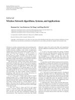
sition 575. Figure 8 shows the 2D spectrum of the MCARM
radar data [9] at range cell 200, we can clearly note the mono-
static STAP clutter ridge. Its slope is approximately β
 1.
3
The slow convergence is mainly due to the high-input eigenvalue spread
of the STAP covariance matrix which is a problem inherent in adaptive
algorithms [14](λ
max
 CNR + 10 log(NM)(dB)), see Figure 4.
0 100 200 300 400 500 600
Number of training samples
40
35
30
25
20
15
10
5
0
SINR loss (dB)
EC

PAST
PASTd
OPAST
FAPI
Figure 6: SINR loss as a function of the training data support K.
Forgetting factor μ
= 0.99.
0.5 0.4 0.3 0.2 0.100.10.20.30.40.5
Normalized Doppler frequency
45
40
35
30
25
20
15
10
5
0
SINR loss (dB)
Optimal
EC
FAPI
LSMI δ
= 10σ
2
Figure 7: SINR loss as a function of the normalized Doppler fre-
quency.
Figure 9 depicts power versus range at pulse 1, the first ra nge
cells represent transmit leakage [16]andarenotusedfor

our simulations. In this example, only range cells from 200
to 600, N
= 14 channels, and M = 16 pulses are used for
the performance evaluation. We inject artificially a target at
range cell 290 at angle bin 65 corresponding to 0
◦
(broad-
side) and normalized Doppler frequency of 0.3 with ampli-
tude 0.00003. Because of the nonavailability of the noise level
of the antenna in the MCARM data, we prefered to use the
modified sample matrix inversion (MSMI) as defined below:
η
=


w
H
x


2
w
H

Rw
. (22)
H. Belkacemi and S. Marcos 7
1 0.6 0.20.20.61
Sin (azimuth)
0.5

0.4
0.3
0.2
0.1
0
0.1
0.2
0.3
0.4
0.5
Normalized Doppler
55
50
45
40
35
30
25
20
15
10
5
0
Figure 8: Power spectrum for MCARM radar data range cell 200.
0 100 200 300 400 500 600 700
Range cell number
40
30
20
10

0
10
20
30
40
50
Received power (dB)
Figure 9: Output power of MCARM versus range at pulse 1.
Figure 10 shows the eigenspectrum of the sample covariance
matrix, the spectrum does not show a sharp cutoff at the in-
terference rank value as for simulated data. There is a gradual
decrease, this is mainly due to the crabbing ang l e. We choose
arankofr
= 90 corresponding to noise power of −55 dB
4
rather than the rank suggested by Brennan’s rule which is
r
= 14 − (16 − 1) = 29.
Figure 11 shows the MSMI statistics over range. We note
that the target is visible for both EC and FAPI with the same
level of power.
7. CONCLUSION
In this paper, the application of fast recursive subspace algo-
rithms for interference mitigation in STA P radar is consid-
ered. We evaluate the performance of a recently developed
4
The choice of this noise power level corresponds to realistic values [9].
0 50 100 150 200 250
Eigenvalue index
80

70
60
50
40
30
20
10
0
10
Eigenvalue (dB)
Figure 10: Eigenspectrum using the sample covariance matrix of
the MCARM data.
240 250 260 270 280 290 300 310 320 330 340
Range cell
30
20
10
0
10
20
30
Power (dB)
EC
FAPI
Figure 11: MSMI statistics over range for EC and FAPI, injected
target at range cell 290.
fast subspace algorithm known as FAPI. The results of sim-
ulation using synthetic data and measured data show that
FAPI algorithm approaches the same performance of the EC
with a linear computation complexity (O(NMr)) rather than

(O(NM)
3
) for the EC.
REFERENCES
[1] R. Klemm, Space-Time Adaptive Processing: Principles and Ap-
plications, vol. 9 of IEE Radar, Sonar, Navigation and Avionics,
IEE Press, London, UK, 2000.
[2] M. I. Skolnik, Radar Handbook, McGraw-Hill, New York, NY,
USA, 1990.
[3] L. E. Brennan and L. S. Reed, “Theory of adaptive radar,” IEEE
Transactions on Aerospace and Electronic Systems,vol.9,no.2,
pp. 237–252, 1973.
8 EURASIP Journal on Applied Signal Processing
[4] A. Haimovich, “Eigencanceler: adaptive radar by eigenanalysis
methods,” IEEE Transactions on Aerospace and Electronic Sys-
tems, vol. 32, no. 2, pp. 532–542, 1996.
[5] Y. Hua, Y. Xiang, T. Chen, K. Abed-Meraim, and Y. Miao, “A
new look at the power method for fast subspace tracking,” Dig-
ital Signal Processing, vol. 9, no. 4, pp. 297–314, 1999.
[6] R. Badeau, B. David, and G. Richard, “Fast approximated
power iteration subspace tracking,” IEEE Transactions on Sig-
nal Processing, vol. 53, no. 8, pp. 2931–2941, 2005.
[7] B. Yang, “Projection approximation subspace tracking,” IEEE
Transactions on Signal Processing, vol. 43, no. 1, pp. 95–107,
1995.
[8] K. Abed-Meraim, A. Chkeif, and Y. Hua, “Fast orthonormal
PAST algorithm, ” IEEE Signal Processing Lette rs, vol. 7, no. 3,
pp. 60–62, 2000.
[9] B. Himed, “MCARM/STAP data analysis,” Tech. Rep. AFRL-
SN-RS-TR-1999-48, Air Force Research Laboratory, Dayton,

Ohio, USA, May 1999, Vol II.
[10] J. Ward, “Space-time adaptive processing for airborne radar,”
Tech. Rep. 1015, MIT Lincoln Laboratory, Lexington, Mass,
USA, December 1994.
[11] P. G. Richardson, “STAP covariance matrix structure and its
impact on clutter plus jamming suppression solutions,” Elec-
tronics Letters, vol. 37, no. 2, pp. 118–119, 2001.
[12] Y. Hua, “Asymptotical orthonormalization of subspace ma-
trices without square root,” IEEE Signal Processing Magazine,
vol. 21, no. 4, pp. 56–61, 2004.
[13] Y. Jung-Lang, “A novel subspace tracking using correlation-
based projection approximation,” Signal Processing, vol. 80,
no. 12, pp. 2517–2525, 2000.
[14] M. Kamenetsky and B. Widrow, “A variable leaky LMS adap-
tive algorithm,” in Proceedings of the IEEE conference of the 38th
Asilomar on Signals, Systems and Computers, vol. 1, pp. 125–
128, Pacific Grove, Calif, USA, November 2004.
[15] Y. L. Kim, S. U. Pillai, and J. R. Guerci, “Optimal loading fac-
tor for minimal sample support space-time adaptive radar,” in
Proceedings of the IEEE International Conference on Acoustics,
Speech and Signal Processing (ICASSP ’98), vol. 4, pp. 2505–
2508, Seattler, Wash, USA, May 1998.
[16] J. S. Goldstein, I. S. Reed, and P. A. Zulch, “Multistage partially
adaptive stap cfar detection algorithm,” IEEE Transaction on
Aerospace and Electronic Systems, vol. 35, no. 2, pp. 645–662,
1999.
Hocine Belkacemi wasborninBiskra,Al-
geria. He received the Engineering degree
in electronics from the Institut National
d’Electricit

´
e et d’Electronique (INELEC),
Boumerdes, Algeria, in 1996, the Magist
´
ere
degree in electronic systems from
´
Ecole Mil-
itaire Polytechnique, Bordj El Bahri, Alge-
ria, in 2000, and the M.S. (DEA) degree in
control and signal processing, Universit
´
ede
Paris-Sud XI, Orsay, France, in 2002. He is
currently pursuing the Ph.D. degree in the field of signal process-
ing at the Signals and Systems Laboratory (LSS) at Sup
´
elec, Gif-sur-
Yvette. His research interests include array signal processing with
application to radar, detection and estimation, and model selec-
tion.
Sylvie Marcos received the Engineer degree
from the Ecole Centrale de Paris (1984) and
both the Doctorate (1987) and the Habil-
itation (1995) degrees from the Paris-Sud
XI University, Orsay, France. She is Direc-
tor of Research at the National Center for
Scientific Research (CNRS) and works in
the Signals and Systems Laboratory (LSS)
at Sup

´
elec, Gif-sur-Yvette, France. Her main
research interests are presently array pro-
cessing, spatiotemporal signal processing (STAP) with applications
in radar and radio communications, adaptive filtering, linear and
nonlinear equalizations, and multiuser detection for CDMA sys-
tems.