Báo cáo hóa học: " Blind Mobile Positioning in Urban Environment Based on Ray-Tracing Analysis" ppt
Bạn đang xem bản rút gọn của tài liệu. Xem và tải ngay bản đầy đủ của tài liệu tại đây (1.1 MB, 12 trang )
Hindawi Publishing Corporation
EURASIP Journal on Applied Signal Processing
Volume 2006, Article ID 38989, Pages 1–12
DOI 10.1155/ASP/2006/38989
Blind Mobile Positioning in Urban Environment
Based on Ray-Tracing Analysis
Shohei Kikuchi,
1
Akira Sano,
1
and Hiroyuki Tsuji
2
1
School of Integrated Design Engineering, Faculty of Science and Technology, Keio University, 3-14-1 Hiyoshi Kohoku-ku,
Yokohama, Kanagawa 223-8522, Japan
2
Wireless Communications Department, National Institute of Information and Communications Technology (NICT),
3-4 Hikarino-Oka, Yokosuka, Kanagawa 239-0847, Japan
Received 1 June 2005; Revised 27 October 2005; Accepted 13 January 2006
A novel scheme is described for determining the position of an unknown mobile terminal without any prior information of
transmitted signals, keeping in mind, for example, radiowave surveillance. The proposed positioning algorithm is performed by
using a single base station with an array of sensors in multipath environments. It works by combining the spatial characteristics
estimated from data measurement and ray-tracing (RT) analysis with highly accurate, three-dimensional terrain data. It uses two
spatial parameters in particular that characterize propagation environments in which there are spatially spreading signals due to
local scattering: the angle of arrival and the degree of scattering related to the angular spread of the received signals. The use of RT
analysis enables site-specific positioning using only a single base station. Furthermore, our approach is a so-called blind estimator,
that is, it requires no prior information about the mobile terminal such as the signal waveform. Testing of the s cheme in a city of
high density showed that it could achieve 30 m position-determination accuracy more than 70% of the time even under non-line-
of-sight conditions.
Copyright © 2006 Hindawi Publishing Corporation. All rights reserved.
1. INTRODUCTION
Interest in determining the position of wireless terminals
has been growing rapidly for a number of wireless applica-
tions, such as location-based services, navigation, and secu-
rity. In the United States, for example, the Federal Communi-
cations Commission (FCC) requires wireless carriers imple-
menting enhanced 911 (E-911) service to provide estimates
of a caller’s location within a given accuracy, for instance,
wireless E-911 callers have to be located w ithin 50 m of their
actual location at least 67% of the time [1–3]. In Japan, there
is a need to determine the locations of illegal wireless ter-
minals on vehicles that are interfering with wireless commu-
nication systems [4]. Position determination is also needed
for radiowave surveillance. The most widely used position-
determination scheme is the global positioning system (GPS)
[5]. Although it can be used to determine the locations of
things highly accurately, existing handsets have to be modi-
fied to function as a GPS receiver, and it does not work un-
less the mobile terminal has a line-of-sig ht (LOS) path to the
satellites [2]. Thus, it is not applicable to the detection of a
nonsubscriber such as the radiowave surveillance.
In a few decades, the use of array antennas is receiv-
ing much attention through the efficient use of information
carried in the spatial dimension [1, 6]. More and more mo-
bile positioning schemes using array antenna employed at a
high base station have been investigated as the number of
cellular handset subscribers increases. Until now, a number
of conventional position-determination methods have been
based on trilateration, which combines the received signal
strength (RSS), time-of-arrival (TOA), time-delay-of-arrival
(TDOA), and/or angle-of-arrival (AOA) of signals received a t
three receivers, for example, see [7–10]. This approach also
depends on there being an LOS path between each receiver
and transmitter, which is difficult to observe in urban envi-
ronments since a non-LOS (NLOS) condition significantly
degrades positioning accuracy. Although some NLOS miti-
gation stra tegies can partly improve accuracy by exploiting a
priori knowledge or using a sensor network to a certain ex-
tent [11, 12], the propagation characteristics greatly depend
on the measurement area and the location of the transmitters
and receivers.
On the other hand, database correlation methods, so-
called fingerprint methods, have been showing better detec-
tion capability rather than the trilateration in the last couple
of years, see [13–16] and the references therein. The received
signal fingerprints, such as RSS, TDOA, and angular profile,
are stored as a database by actual measurement in a testing
2 EURASIP Journal on Applied Signal Processing
area, and the estimated location is obtained by minimizing
the Euclidean distance between a sample signal vector a nd
the location fingerprints in the database. This site-specific
technique is especially popular in indoor location systems
such as existing wireless local area network (WLAN) infras-
tructure [14]. The straightforward extension to outdoor po-
sitioning in general cellular systems is unrealistic considering
an immense amount of time and effort to make a database
[16]. Furthermore, the dynamic nature of the outdoor radio
environments makes fingerprint methods infeasible. Instead
of the database made from measurement data, a model-based
approach is promising for outdoor positioning, for example,
the use of ray-tracing (RT) analysis that the radiowave prop-
agation in a testing area is virtually simulated by modeling
three-dimensional (3D) terrain data and propagation laws.
Ahonen and Eskelinen virtually predicted the site-specific
fingerprints of a testing area by using the RT analysis, and
compared RSSs of received signals with those of the RT anal-
ysis results obtained at 7 base stations (a ser ving cell and 6
strongest neighbors) [13]. Basically, however, the use of the
RSSs is not adequate to the applications such as surveillance
of illegal wireless terminals and emergency calls from non-
subscribers, since the RSS estimation needs prior informa-
tion of transmitted signals [10]. Furthermore, using fewer
base stations is important from the economic standpoint.
Although a positioning algorithm with a single base station
employing sensors of array was proposed [17], it utilized the
temporal information of impinging signals that also require
prior knowledge of transmitted signals [9, 18].
This work presents a novel positioning method for use in
multipath environments, which has three important features
as follows.
(i) It uses a “blind algorithm,” that is, it needs no prior
information about the transmitted signal, such as its
signal waveform.
(ii) It is site-specific in that it takes the propagation envi-
ronment into consideration by using RT analysis, and
pinpoints the location of a terminal using only a single
base station.
(iii) It exploits the characteristics of radiowave propagation
in urban environments considering a local scattering
model.
The algorithm consists of two steps. First, the parameters
characterizing the locations in the testing area (defined later)
are experimentally estimated from received signals. Second,
the RT simulations are virtually conducted for calculating
the parameters corresponding to those in the measurement
data analysis, and the estimated location is determined by
matching with the experimentally estimated parameters. The
preliminary calculation of the RT analysis reduces the com-
putational load; however, note that the use of the RT anal-
ysis makes a difference from the conventional fingerprint
methods in that the fingerprint does not always have to be
stored in advance. Further more, one of the notable features
of the proposed algorithm is to give a blind algorithm in or-
der to meet more variable requirements of positioning issues
such as surveillance of illegal wireless terminals as mentioned
Scattering circle
Base station
Mobile station
Local
scatterers
Figure 1: Conceptual diagram of local scattering.
above. The estimation of only spatial parameters realizes
the blind algorithm, while temporal parameter estimation
needs prior information of signal waveform [18]. Those us-
ing code-division multiple access (CDMA), like those de-
scribed by Caffery and St
¨
uber [7], are also considerable for
future communication systems, and the proposed position-
ing algorithm can be applied to the narrowband CDMA sys-
tems, for example, IS-95 [19], if code information for dis-
preading is known in advance. Another feature is to model
the received signal based on a local scattering model that as-
sumes scattering only in the vicinity of a mobile or some re-
flectors, for example, see [20, 21]. This signal model is suit-
able for the propagation environments of urban areas with
a high base station and a low mobile terminal. Then in ad-
dition to AOAs of the received signals, this work introduces
a new spatial parameter indicating the degree of scattering
(DOS) related to the angular spread under the assumption
of the local scattering model, like in Figures 1 and 2.The
two parameters of AOA and DOS are used for pinpointing
the location without any information of transmitted signal
waveform. The DOS is related to a parameter derived from
the first-order approximation of received signal model [20],
and the theoretical performance of the DOS will be also de-
rived in this paper. The matching of these two parameters
dramatically mitigates the computational burden, compared
to the case that angular profile between
−π/2 <θ<π/2 itself
is used for matching [22]. Furthermore, RT analysis [23]us-
ing highly accurate, 3D terrain data realizes site-specific posi-
tioning using only a single base station. Note that the RT an-
alyzer follows the fundamental property of radiowave prop-
agation, for example, geometrical optics (GO) and uniform
theory of diffraction (UTD) [24].
In this paper, the effectiveness of the proposed position-
ing method is evaluated through experimental data analysis
measured at Yokosuka City in Japan, and the results show
that the combination of measurement data and RT analysis
and exploitation of the AOA and DOS prominently improves
the positioning accuracy although the test range is limited
to approximately 500 m
× 500 m. This paper is organized as
follows. Section 2 outlines the basic concept of the proposed
position-determination scheme. The method for estimating
Shohei Kikuchi et al. 3
Transmi tt er
Base station
Multiple scattering
signals
Local scattering
circles
Figure 2: Local scattering on reflectors.
the AOA and DOS in the exper imental data analysis and the
theoretical behavior of the DOS are described in Section 3.
Section 4 mentions the fundamental property of the RT anal-
ysis and how to exploit the parameters corresponding to the
AOA and DOS from the RT analysis result. The parameter
estimation results obtained through experimental data anal-
ysis and the positioning accuracy of the proposed algorithm
are discussed in Section 5.WeconcludeinSection 6 with a
brief summary.
2. CONCEPT OF PROPOSED
POSITION-DETERMINATION SCHEME
2.1. Local scattering model and parameters
characterizing terminal location
Suppose that a transmitter in a general cellular system is
located in low positions outdoors and its scattered signals,
which deteriorate as a result of multipath propagation, are
measured at a receiver mounted on top of a building. If the
receiver is much higher than the transmitters, a local scatter-
ing model, like the one described by Aszt
´
ely and Ottersten
[20], that considers reflections and scattering in the vicinity
of each transmitter is an appropriate model of the received
signals. In such a model, spatially spread signals are observed
at the receiver, as illustrated in Figure 1.However,inprac-
tical situations, especially under NLOS conditions between
the transmitter and receiver, which is the case dealt with
throughout this paper, the spread signals are usually mea-
sured after propagating along several routes, as illustrated in
Figure 2. As a result, the received signal is expressed as the
summation of several local scatterers on some reflections. For
example, if there is an LOS between a transmitter and a re-
ceiver, the transmitter lies along the AOAs of the direct paths
to multiple base stations. If there is no LOS, the locations of
terminals cannot always be identified by using the AOA esti-
mates, making the position-determination more difficult.
Our proposed positioning method, using a single array of
sensors, uses two particular spatial parameters, the AOA and
DOS, to determine the location of a terminal. These param-
eters represent the path characteristics, which depend on the
propagation environment between the transmitter and re-
ceiver. The signals can be discriminated using the DOSs, even
if their AOAs are the same. Estimation of these two parame-
ters and the relationship between the angular spread and the
bit error rate (BER) are described elsewhere [25, 26].
2.2. Positioning method using ray-tracing analysis
The AOA and DOS estimated from the received sig nals are
not sufficient for determining the location of a mobile termi-
nal with a single base station, since the location of the mo-
bile is not always determined by such trilateration because of
an NLOS condition and/or multipath propagation. We also
have to use RT analysis. Using an RT simulator, we can vir-
tually analyze the radiowave propagation using the given ter-
rain data and some propagation parameters such as coeffi-
cients of reflection and diffraction. Since the rendering of ge-
ographical information has been attracting much attention,
this technology should become widely used in a variety of
applications in the near future. This work thus uses the RT
analysis with highly accurate 3D terrain data around the test-
ing area to estimate the location of a terminal, by comparing
with the results of the two spatial parameters from both ex-
perimental and RT analyses. In the RT analysis, these param-
eters can be calculated from all the rays between a transmitter
and receiver as shown in Figure 3. In addition, the estimated
AOAs and DOSs are virtually measured at all outdoor loca-
tions (e.g., every 10 m). The calculated AOAs and DOSs in
the RT analysis are used for estimating the location of the
terminal. Let
θ
k
and η
k
, k = 1, , K, denote, respectively,
the estimated AOA and DOS of the kth scatterer obtained
in the experimental analysis. Similarly, let θ
(RT)
k
(X, Y)and
η
(RT)
k
(X, Y), k = 1, , K, be, respectively, the estimates in
the RT analysis, where (X,Y) indicates the Cartesian coor-
dinate of the pseudotransmitters inside the testing area D.
Note that K is the number of scatterers in Figure 2, not that
of the total rays. We estimate the location of a terminal using
a cost function:
F(X,Y)
=
K
k=1
(1 − ν)
θ
k
− θ
(RT)
k
(X, Y)
2
+ ν
η
k
− η
(RT)
k
(X, Y)
2
1/2
,
(1)
where θ
k
is the radian measure, and 0 ≤ ν ≤ 1 is a weighting
factor that indicates the ratio between the correlation of the
AOAs and DOSs. The (X, Y) minimizing this cost function is
taken as the estimated position. That is,
X,
Y
= arg min
X,Y ⊆D
F(X,Y), (2)
where (
X,
Y) is the estimated position. The diagram of
this algorithm is illustrated in Figure 4. Combining the re-
sults for multiple signals from different directions enables to
use the multipath propagation, conventionally regarded as a
4 EURASIP Journal on Applied Signal Processing
Tx
Rx
Figure 3: 3D terrain data around testing area and RT analysis. A
number of rays from a transmitter (Tx) reach a receiver (Rx) via
different reflections and diffractions.
problem to be avoided, to pinpoint the locations of mobile
terminals using only a single receiver even under NLOS con-
ditions.
Remark 1. This work deals with the position determination
of one mobile terminal using a single base station. If the
number of users is more than one, then the total number
of scatterers is K
T
=
I
i=1
K
i
,whereI denotes the number
of transmitted sources, and K
i
is the number of scatterers
generated from the ith source. In order to determine the po-
sition of the mobiles, we need the identification of
{K
i
}
I
i
=1
and the association, that is, which transmitted source the kth
scatterer belongs to. This problem is called “source associa-
tion.” As one idea to solve the problem, Yan and Fan pro-
posed an algorithm for categorizing the distinc t K
T
AOAs
into I groups in the case that the ith group includes K
i
coher-
ent signals [27]. Note that the total number of scatterers K
T
has to meet the condition M>K
T
,whereM is the number of
sensors of array. Suppose I
= 1andK
T
= K
1
= K through-
out this paper.
3. DATA MODEL AND PARAMETER ESTIMATION
This section describes the received signal model for multi-
path environments, like the one illustrated in Figure 2,based
on the local scattering model. We also mention the estima-
tion of the AOA and DOS, and statistically derive the physical
properties of the DOS.
3.1. Signal model considering local scattering
The received signal model is expressed as the summation
of multiple local scatterers [25, 26, 28]. We assume that
the transmitter is stationary during observation and that
the time dispersion introduced by the multipath propaga-
tion is small compared to the reciprocal of the bandwidth of
the transmitted signals. An M-element uniform linear array
(ULA) is used as the base station; it is mounted on top of a
high building. A flat Rayleigh fading narrowband channel is
considered. The received signal consists of K scatterers; the
number depends on the physical propagation phenomena,
such as reflection and diffraction:
x(t)
=
K
k=1
L
k
l=0
β
kl
a
θ
k
+
θ
kl
s
t − τ
kl
+ n(t)(3)
≈
K
k=1
L
k
l=0
α
kl
a
θ
k
+
θ
kl
s
k
(t)+n(t), (4)
where L
k
and β
kl
are the total number of rays associated w ith
the kth scatterer and complex amplitude of the lth ray in the
kth scatterer, respectively. s
k
(t) is the signal of the kth scat-
terer , and n(t) is an additive white Gaussian noise (AWGN)
vector. We assume that the array response vector is perfectly
known from calibration. The mth factor of a(θ
k
) is expressed
as a
m
(θ
k
) = exp{j2πdsin θ
k
/λ} for ULAs. The quantities θ
k
and θ
k
+
θ
kl
represent the nominal AOA of the kth scatterer
and the arrival angle of the lth ray in the kth scatterer, respec-
tively. This means that
|β
k0
| is sufficiently large compared to
|β
kl
| under the condition that the kth scatterer includes a di-
rect path, while
|β
k0
| is at almost the same level as |β
kl
| if the
scatterer results from reflections. Note that this model covers
both LOS and NLOS conditions. Assuming narrowband sig-
nals, the time delay of the scattered signals is included in the
phase shift [20]. Thus, given the definitions s
k
(t)
= s(t −τ
k0
)
and Δτ
kl
= τ
kl
−τ
k0
,weobtain(4)from(3) using an approx-
imation:
s
t − τ
kl
≈ s
k
(t)exp
− j2πf
c
Δτ
kl
,
α
kl
= β
kl
exp
− j2πf
c
Δτ
kl
, k = 1, , K.
(5)
3.2. Scattering parameter
3.2.1. Definition
It is impossible to identify all the unknown parameters in (4)
since the number of scattered signals, L
k
, is too large and un-
countable. Therefore, a number of statistical approaches to
deal with the scattering model have been so far proposed.
For instance, the standard deviation of the distributed rays
is estimated by the weighted subspace fitting [21], which re-
quires heavy computational load. On the other hand, assum-
ing that the rays are independent and identical ly distributed
with phases uniformly distributed over [0, 2π], and that the
number of rays is sufficiently large, the central limit theorem
may be used to approximate the elements of the spatial signa-
ture as complex Gaussian random variables. Thus, (4)canbe
approximated using a first-order Taylor expansion under the
assumption that the angular spread is small, that is,
|
θ
kl
|→0
[20, 21]:
x(t)
≈
K
k=1
L
k
l=0
α
kl
a
θ
k
+
θ
kl
d
θ
k
s
k
(t)+n(t)
=
K
k=1
γ
k
a
θ
k
+ φ
k
d
θ
k
s
k
(t)+n(t)
=
K
k=1
a
θ
k
+ ρ
k
d
θ
k
s
k
(t)+n(t),
(6)
Shohei Kikuchi et al. 5
Measurement
data analysis
(Section 3)
3D data around
testing area
Ray-tracing
analysis
(Section 4)
Estimated
location
(
X,
Y)
x(t)
(X, Y)
F(X,Y)
θ , η
θ
(RT)
(X, Y)
η
(RT)
(X, Y)
Figure 4: Diagram of proposed positioning algorithm.
where d(θ)
=
∂a(θ)/∂θ,and
γ
k
=
L
k
l=0
α
kl
, φ
k
=
L
k
l=0
α
kl
θ
kl
. (7)
Including γ
k
in s
k
(t) as the complex amplitude, we define
ρ
k
= φ
k
/γ
k
and s
k
(t)
= γ
k
s
k
(t). Due to the definitions of
γ
k
and φ
k
of (7), the identification of the number of the rays
in a scatterer L
k
is unnecessar y. The model is then consistent
with flat Rayleigh fading since the magnitude of each element
of the spatial signature has a Rayleigh distribution. There are
three unknown parameters in (6), θ
k
, ρ
k
,ands
k
(t); ρ
k
has
been discussed elsewhere [20, 25]. Actually, however, ρ
k
tem-
porally fluctuates as a result of multipath fading in practical
situations. Thus, we define a new parameter called the “de-
gree of scattering (DOS)” using the expectations of the abso-
lute values of φ
k
and γ
k
as
η
k
=
E
φ
k
E
γ
k
,(8)
where E
{·} denotes the expectation. This parameter η
k
is
theoretically relevant to the angular spread of the kth scat-
terer, and the detailed behavior of the parameter is discussed
in Section 3.2.3. The DOS can be estimated without any prior
information such as signal waveform, and the identification
ofbothAOAandDOSisappropriateforfingerprint to deter-
mine the location under the assumption of the local scatter-
ing model.
3.2.2. Parameter estimation method
To estimate the AOAs and DOSs, we assume that the number
of scatterers K is correctly estimated in advance. Although
eigenvalue-based nonparametric source number detection
methods such as the Akaike information criterion (AIC) and
minimum description length (MDL) criterion are commonly
used [29], they does not work well in the presence of angular
spread. Recently, robust source number estimators have been
described elsewhere, for example, [30], based on the gener-
alized maximum-likelihood-ratio test principles, that work
well even for slightly scattered signals. The K nominal AOAs
are estimated from correlated sources by an AOA localizer
based on TLS-ESPRIT [31] with a spatial smoothing [32],
under the assumption that the angular distribution for a scat-
terer is symmetrical. The DOSs are obtained using the least-
squares (LSs) method:
s
k
(t), ρ
k
=
arg min
s
k
(t),ρ
k
J(t), (9)
where J(t) is the cost function used to estimate
s
k
(t)andρ
k
,
J(t)
=
x(t) −
K
k=1
a
θ
k
+ ρ
k
d
θ
k
s
k
(t)
2
. (10)
The K sets of DOS are recursively calculated using only the
x(t) of the received signals as follows.
Step 1. Obtain
θ
k
, k = 1, , K.
Step 2. Initialize K-column vector,
ρ
(0)
= [0, ,0]
T
,where
ρ
(i)
denotes the ith iteration of ρ = [ ρ
1
, , ρ
K
]
T
.
Step 3. Calculate ML estimate
s
k
(t):
s(t) =
V
H
V
−1
V
H
x(t), (11)
where
V =
K
k=1
a
θ
k
+ ρ
k
d
θ
k
,
s(t) =
s
1
(t), ,
s
K
(t)
T
.
(12)
Step 4. Estimate ρ
k
using an LS approach that minimizes the
following cost function:
J
2
= E
x(t) − x(t)
2
, (13)
where
x(t) =
K
k=1
a
θ
k
+ ρ
k
d
θ
k
s
k
(t) = A
Se + D
Sρ,
A
=
a
θ
1
, , a
θ
K
,
D
=
d
θ
1
, , d
θ
K
,
S = Diag
s
1
(t), ,
s
K
(t)
,
ρ
=
ρ
1
, , ρ
K
T
,
e
= [1, ,1]
T
.
(14)
6 EURASIP Journal on Applied Signal Processing
Diag{·}is a diagonal matrix whose diagonal elements are
{·}. Thus, the cost function (13) can be reobtained as
J
2
= E
A
Se + D
Sρ − x(t)
2
=
E
D
Sρ − z
2
, (15)
where z = x(t) − A
Se.
Step 5. Repeat Steps 4 and 5 until
ρ converges.
Step 6. Derive
|γ
k
| under the condition E{s
k
(t)s
∗
k
(t)}=1:
E
s
k
(t)s
∗
k
(t)
=
E
γ
k
s
k
(t)s
∗
k
(t)γ
∗
k
=
γ
k
2
. (16)
Step 7. Calculate
φ
k
=|γ
k
||ρ
k
|.
Step 8. Repeat the above steps for every time slot (includ-
ing enough samples). Determine expectations E
{|γ
k
|} and
E
{|
φ
k
|} by temporal averaging, and obtain η
k
from (8).
3.2.3. Theoretical behavior of scattering parameter
The theoretical performance of the proposed parameter η
k
is
considered to clarify its physical meaning. The resultant for-
mulations are applied to the RT analysis. First, the theoretical
behavior of the expectations E
{|γ
k
|} and E{|φ
k
|} are derived
for LOS and NLOS conditions, respectively.
From (16),
|γ
k
| means the amplitude envelope of the
signal received at the base station, and it varies based on
Nakagami-Rice fading, which has a probability density func-
tion (pdf) that follows the Ricean distribution. Note that
Nakagami-Rice fading includes Rayleigh fading as a special
case. Since the phase of α
kl
changes randomly during ob-
servation, the expected values and variances of
{α
kl
} and
{α
kl
} can be expressed, respectively, as
E
α
Re
=
E
α
Im
=
0,
Var
α
Re
=
E
α
2
Re
=
α
kl
2
2
,Var
α
Im
=
Var
α
Re
,
(17)
where [
·]
Re
and [·]
Im
denote, respectively, the real and imag-
inary parts, and Var
{·} is the variance. Let A
2
k
/2andμ
2
k
=
L
k
· Var{α
Re
}=L
k
· Var{α
Im
} be, respectively, the power of
the main wave and scattered waves. The Ricean factor is de-
fined as the ratio between their powers [24]:
K
k
=
A
2
k
2μ
2
k
. (18)
Basically, the propagation scenarios can be classified into
LOS and NLOS conditions depending on Ricean factor K
k
.
We consider the performance of the DOS in both cases. Since
|γ
k
| follows the Ricean distribution, the expectation E{|γ
k
|}
is
E
γ
k
=
π
2
μ
k
exp
− K
k
M
3
2
;1;K
k
, (19)
where M(
·) denotes Kummer’s confluent hypergeometric
function [33]. The detailed derivation of (19) is given in the
appendix. When K
k
1, the pdf of |γ
k
| is an approximately
Gaussian distribution since the scattered component orthog-
onal to the main wave can be neglected. The expected value
of
|γ
k
| can be approximated as
E
γ
k
≈
A
k
. (20)
On the other hand, without a high-powered main wave, that
is, under NLOS conditions, the level of the scattered waves
is almost the same as that of the main wave. Thus, we define
μ
2
k
= A
2
k
/2+μ
2
k
as the total wave power including the main
wave. Since the pdf of
|γ
k
| is approximated by a Rayleigh dis-
tribution, the expected value of
|γ
k
| can be then expressed
as
E
γ
k
≈
π
2
μ
k
=
π
2
A
2
k
2
+ μ
2
k
=
π
2
μ
k
K
k
+1. (21)
Next, the behavior of φ
k
is considered. From (7), the real
and imaginary parts of φ
k
are, respectively,
φ
Re,k
=
L
k
l=1
α
Re,k,l
θ
kl
, φ
Im,k
=
L
k
l=1
α
Im,k,l
θ
kl
, (22)
where
θ
k0
= 0 without loss of generality. Under the assump-
tion that
θ
kl
and α
kl
have no correlation, the pdfs of both
φ
Re,k
and φ
Im,k
can be approximated as Gaussian distribu-
tions. The expectations of φ
Re,k
and φ
Im,k
are given, respec-
tively, as
E
φ
Re,k
=
0, E
φ
Im,k
=
0. (23)
Thus, their variances are, respectively,
Var
φ
Re
=
L
k
E
θ
2
E
α
2
Re
=
μ
2
k
σ
2
θ
k
,
Var
φ
Im
=
L
k
E
θ
2
E
α
2
Im
=
μ
2
k
σ
2
θ
k
,
(24)
where σ
θ
k
denotes the standard deviation of the angular dis-
tribution, the so-called angular spread [21]. Since the dis-
tributions of φ
Re
and φ
Im
are Gaussian, the pdf of |φ|=
φ
2
Re
+ φ
2
Im
follows the Rayleigh distribution. From (24), the
expected value of
|φ
k
| is
E
φ
k
=
π
2
μ
k
σ
θ
k
. (25)
As shown by (8), the DOS is defined as the ratio between
E
{|γ
k
|} and E{|φ
k
|}. Under the condition K
k
1, that is,
an LOS condition, we derive the parameter η
LOS,k
using (20)
and (25):
η
LOS,k
=
E
φ
k
E
γ
k
≈
π
2
μ
k
σ
θ
k
A
k
=
π
4
σ
θ
k
K
k
, (26)
where η
LOS,k
is proportional to σ
θ
k
and inversely proportional
to
K
k
. Furthermore, when the level of the main wave is al-
most the same as that of the scattered waves, which occurs
mainly under NLOS conditions, η
NLOS,k
is given from (21)
and (25):
η
NLOS,k
=
E
φ
k
E
γ
k
≈
σ
θ
k
K
k
+1
, (27)
Shohei Kikuchi et al. 7
where η
NLOS,k
is pr oportional to σ
θ
k
, and inversely propor-
tional to
K
k
+ 1. Equations (26)and(27) mean that the
DOS η
k
depends on the Ricean factor K
k
and angular spread
σ
θ
k
of each AOA. This means the larger the DOS is, the more
widely the impinging kth signal is distr ibuted, and vice versa.
Thus, the DOS is an efficient criterion for describing the de-
gree of scattering.
4. RAY-TRACING ANALYSIS
Section 2 described the basic procedure of the proposed po-
sitioning method. In our scheme, the AOAs and DOSs ob-
tained by practical data analysis are compared w ith those by
RT analysis using the cost function of (1). This sect ion de-
scribes how the parameters are calculated in the RT analysis.
We use highly accurate, 3D terrain data for the experimen-
tal area. The data is collected for approximately 20 layers per
material including the conditions of the dielectric properties
regarding the materials of reflectors and the 3D coordinates
obtained within a height accuracy of
±25 cm. The RT analy-
sis follows propagation rules such as the GO and UTD [24],
and enables us to determine the position of terminals accu-
rately using site-specific information for the measurement
area.
In the analysis, the receiver is virtually located in the
same place as in the experiment described in the next section,
and the waves propagate following the geometr ic laws of ra-
diowave propagation. We use the ray-launching method [23]
for our RT simulator as it is more tractable and computa-
tionally reasonable than the other commonly used approach,
that is, the imaging method. The ray-launching method ra-
diates a ray at every angle Δθ from a transmitter, and the
path is traced through reflection, transmission, and diffrac-
tion points, while the imaging method traces a ray reflec-
tion and transmission route connecting a transmission point
with a reception point by obtaining an imaging point against
a reflection surface. Thus, the implementation of the imag-
ing method is unrealistic as the terrain data become huge.
As a result of the RT analysis, an angular profile can be ob-
tained like that shown in Figure 5, which indicates the valid-
ity of modeling the received signal using the local scattering
model. From the profile, a scatterer is defined as a signal clus-
ter including a nominal ray above 30 dB and rays 10 degrees
around when the least signal level that the receiver detects
is set at 0 dB. Therefore, Figure 5 can be regarded as a case
of K
= 2. The angular spread of each scatterer is calculated
using the second-order statistics:
σ
(RT)
θ
k
=
1
L
k
L
k
l
=1
θ
(RT)
kl
−
¯
θ
(RT)
k
2
·
P
(RT)
kl
¯
P
(RT)
k
, (28)
where
¯
θ
(RT)
k
and
¯
P
(RT)
k
are, respectively, the nominal AOA and
its power, θ
(RT)
kl
and P
(RT)
kl
are the AOAs and powers of the
scattered waves, respectively, and L
k
is the total number of
both nominal and scattered waves. The theoretical behavior
of the DOS derived above says that the DOS depends on the
standard deviation of the scattered sig nals and the Ricean
50403020100−10−20−30−40−50
Angle (deg)
0
10
20
30
40
50
DOA spectrum (dB)
1st scatterer 2nd scatterer
Additive noise
Figure 5: Example of angular profile by RT analysis (K = 2). It is
shown that some rays are launched from the Tx and reflected on the
reflector. At the end of the process, a fewer number of rays may be
received at the Rx.
factor. Thus, the DOS is also derived from those parame-
ters even in the RT analysis. The Ricean factor is given by
K
(RT)
k
=
¯
P
(RT)
k
/2
L
k
l
=1
P
(RT)
kl
since it is the ratio between the
powers of the main and scattered waves. Using (26), (27), and
(28), we can obtain the DO S under LOS conditions by
η
(RT)
LOS,k
=
π
4
σ
(RT)
k
K
(RT)
k
, (29)
and under NLOS conditions by
η
(RT)
NLOS,k
=
σ
(RT)
k
K
(RT)
k
+1
. (30)
Note that determining whether the mobile terminal is at an
LOS or NLOS location is obvious in the RT simulations. We
can thus obtain K
(RT)
, θ
(RT)
k
,andη
(RT)
k
for all points in the 3D
terrain and use for pinpointing the location of terminals, in
combination with the results of the experimental data analy-
sis.
5. EXPERIMENTAL DATA ANALYSIS AND
POSITION-DETERMINATION ACCURACY
We now consider the application of the parameter estima-
tion method described above to experimental data measured
using array antennas. The accuracy of the proposed position-
determination algorithm based on experimental data analy-
sis is also discussed.
5.1. Experimental conditions
We analyzed data obtained from field testing in Yokosuka
City, Japan, a city with a high housing density. An exper-
imental array used as the base station receiver (Rx) was
mounted on top of a 15 m high building, employing the
ULA with eight-element microstrip patch antenna. The an-
tenna elements were separated by half the wavelength of the
8 EURASIP Journal on Applied Signal Processing
Rx
Tx1
Tx2
Tx3
Tx4
Tx5
Tx6
0(degree)
Figure 6: Map around testing area.
Table 1: Angle, distance, and transmitted power regarding each Tx.
LOS NLOS
Tx1 Tx2 Tx3 Tx4 Tx5 Tx6
Angle (deg) −15.710.60−6.522.954.8
Distance (m)
215 200 100 300 200 210
Power (dBm)
010030 20 30
2.335 GHz carrier frequency. Figure 6 shows a map of the
testing area, and Table 1 summarizes the angles, distances,
and signal powers of the transmitters, which were 1.5 m high.
The transmitters (Tx1-6) were stationary; three of them (Tx1
to Tx3) were at LOS positions, while the others (Tx4 to Tx6)
were at NLOS positions. The transmitted signal was formed
by π/4-shift QPSK modulation. We took 1900 snapshots at
a sample rate of 2 MHz, which meant that the observation
time was only 10
−3
second. The other specifications and the
experimental system are described elsewhere [34]. The data
was collected at the base station. Note that the analysis was
done for one terminal at a time.
5.2. Experimental analysis
The AOAs and DOSs were estimated by using the proce-
dure described in Section 3.2.2. Tables 2 and 3 summarize
the AOAs and DOSs estimated under LOS and NLOS condi-
tions, respectively. We analyzed 1900 sample sig nals, divided
into 19 groups, and calculated E
{|γ
k
|} and E{|φ
k
|} by aver-
aging the estimates for those 19 periods to estimate the DOS,
η
k
.
The previous numerical simulations [26] showed that the
DOS was correlated with the BER of beamformed signals,
which meant that the DOS indicated the degree of scattering.
This is supported by the results shown in Tables 2 and 3.The
DOS of a direct path was much smaller than that of reflected
ones since the definition of the DOS in (26)and(27)says
that the DOS is smaller as the Ricean factor is larger. Thus,
since both AOA and DOS are appropriate parameters for de-
scribing the characteristics of each scatterer, we use them as
the key to obtain the locations of terminals.
5.3. Positioning method and its accuracy
We estimated the location of terminals using the results of
the field testing and RT analysis by the method described in
Section 2. First, using the RT simulator, pseudotransmitters
were positioned at 10 m intervals within about 500 m
×500 m
on the map in Figure 6 and the AOAs and DOSs were esti-
mated for each one. Note that the D O Ss were obtained sepa-
rately for the LOS and NLOS transmitter positions since the
DOSs in the RT analysis behave differently i n (29)and(30).
The results were matched with the experimental analysis re-
sults by using the cost function of (1) with the weighting fac-
tor ν
= 0.5.
Tables 4 and 5 show how accurately the location could
be estimated in terms of probability for 200 trials using tem-
porally different signals from the same point. For example,
the location of Tx4 under NLOS conditions was estimated
within 10 m in 31.5% of the trials, 20 m in 65.0%, and 30 m
in 83.5%. Overall, the results show that positioning accuracy
was within 30 m more than 73.5% of the time, even under
NLOS conditions. These results easily satisfy the E-911 re-
quirements of the FCC that the estimated location of a caller
is within 50 m of the caller’s actual location more than 67%
of the time [2], and they show that our scheme outperforms
other positioning schemes, such as [13, 17].
Shohei Kikuchi et al. 9
Table 2: Parameter estimation results using actual data in LOS conditions.
Tx no. Tx1 Tx2 Tx3
Path no. Path1 Path2 Path1 Path2 Path3 Path1 Path2 Path3
DOA (deg) −15.745.7 −24.610.317.5 −38.80.040.5
DOS
0.0102 0.2942 0.0912 0.0535 0.5013 0.1492 0.0116 0.2239
Table 3: Parameter estimation results using actual data in NLOS conditions.
Tx no. Tx4 Tx5 Tx6
Path no. Path1 Path2 Path3 Path1 Path2 Path1 Path2 Path3
DOA (deg) −18.212.544.8 −29.015.1 −40.13.149.4
DOS
0.0368 0.1674 0.0812 0.0952 0.0715 0.6824 0.1328 0.3972
5.4. Weighting factor and positioning accuracy
To prove the effectiveness of introducing DOS, the position-
ing accuracy was evaluated at different values of the weight-
ing factor ν in (1). Figure 6 shows the relationship between
the probability of accuracy within 20 m and the weighting
factor. The results confirm that introducing DOS, which re-
flects the propagation characteristics, dramatically improved
position-determination accuracy. Although the optimization
of the weighting factor is quite difficult since it depends on
the transmitter location, the results show that the accuracy
was approximately 15% to 40% better when both AOA and
DOS were used than when only AOA was used.
6. CONCLUSION
We have described the novel method for determining the po-
sition of a wireless terminal; it uses a single array antenna
and is suitable for use in multipath environments. It makes
use of two spatial parameters, the ang le of arrival and the de-
gree of scattering, which reflect the path characteristics be-
cause they depend on the propagation environment between
the transmitter and the receiver. These parameters are used
in combination with the results of ray-tracing analysis with
highly accurate 3D terrain data. The key features of our algo-
rithm are that it is “blind,” which needs no prior information
about the transmitted signal such as signal waveform, keep-
ing in mind the application of unknown source detection for
radiowave surveillance. Furthermore, it is based on a local
scattering model considering scattering in the vicinity of a
mobile or some reflectors. We achieved a site-specific scheme
with only a single base station by introducing the ray-tracing
analysis.
Field testing showed that the proposed method was su ffi-
ciently accurate to meet the Federal Communications Com-
mission requirements for mobile terminal position deter-
mination and that it outperformed other positioning al-
gorithms, although the experimental area was only about
500 m
×500 m. This site-specific method can be used in other
locations if only experimental data and 3D terrain data are
available.
APPENDIX
The expectation of
|γ
k
| in (19)isderivedasfollows.Firstwe
define r
=|γ
k
|, and the pdf p(r) follows the Ricean distribu-
tion:
p(r)
=
r
μ
2
k
exp
−
r
2
+ A
2
k
2μ
2
k
I
0
A
k
r
μ
2
k
,(A.1)
where μ
k
= L
k
·Var {α
Re
}=L
k
·Var {α
Im
},andI
0
(·)isazero-
order Bessel function of the first kind [33]. The expectation
of r is expressed as an integra l in terms of r:
E
{r}=
∞
0
r · p(r)dr =
∞
0
r
2
μ
2
k
exp
−
r
2
+ A
2
k
2μ
2
k
I
0
A
k
r
μ
2
k
dr.
(A.2)
This equation can be modified with the following mathemat-
ical formulae using a Gamma function and the Kummer’s
confluent hypergeometric function [33], respectively:
∞
0
x
ξ−1
exp
− a
2
x
2
I
υ
(bx)dx
=
Γ
(ξ + υ)/2
b
υ
2
υ+1
a
ξ+υ
Γ(υ +1)
· M
ξ + υ
2
; υ +1;
b
2
4a
2
,
M(c; d; z)
=
∞
k=0
(c)
k
(d)
k
z
k
k!
= 1+
c
d
z
1!
+
c(c +1)
d(d +1)
z
2
2!
+
c(c +1)(c +2)
d(d +1)(d +2)
z
3
3!
+
···,
(A.3)
where Γ(x) is the Gamma function, M(c; d; z) is the Kum-
mer’s confluent hypergeometric function, and we define
(x)
n
=
Γ(x + n)
Γ(x)
= x(x +1)···(x + n − 1). (A.4)
10 EURASIP Journal on Applied Signal Processing
Table 4: Positioning accuracy in LOS conditions: “Num.” denotes the number of successful estimations within each accuracy up to 200
trials, and “Prob.” is cumulative probability of correct positioning.
Positioning Tx1 Tx2 Tx3
accuracy Num. Prob. Num. Prob. Num. Prob.
Within 10 m 158 79.0% 123 61.5% 181 90.5%
Within 20 m
40 89.0% 49 86.0% 19 100%
Within 30 m
2 100% 28 100% 0 100%
Table 5: Positioning accuracy in NLOS conditions: “Num.” denotes the number of successful estimations within each accuracy up to 200
trials, and “Prob.” is cumulative probability of correct positioning.
Positioning Tx4 Tx5 Tx6
accuracy Num. Prob. Num. Prob. Num. Prob.
Within 10 m 63 31.5% 82 41.0% 19 9.5%
Within 20 m
68 65.0% 77 79.5% 72 45.5%
Within 30 m
36 83.5% 22 90.5% 56 73.5%
10.80.60.40.20
Weighting factor ν
20
40
60
80
100
Probability (%)
Tx1
Tx2
Tx3
(a)
10.80.60.40.20
Weighting factor ν
20
40
60
80
100
Probability (%)
Tx4
Tx5
Tx6
(b)
Figure 7: Positioning accuracy within 20 m in case of changing
weighting factor ν: (a) the result of detecting Tx1 to 3 located at
LOS positions, while (b) shows the detection probability of Tx4 to
6 at NLOS positions.
Substituting x = r, ξ = 3, υ = 0, a = 1/(
√
2μ
k
), and b = A
k
/
μ
2
k
into ( A.3), we obtain (19)from(A.2)as
E
γ
k
=
π
2
μ
k
exp
−
A
2
k
2μ
2
k
M
3
2
;1;
A
2
k
2μ
2
k
. (A.5)
REFERENCES
[1] T.S.Rappaport,J.H.Reed,andB.D.Woerner,“Positionloca-
tion using wireless communications on highways of the futur,”
IEEE Communications Magazine, vol. 34, no. 10, pp. 33–41,
1996.
[2] J.H.Reed,K.J.Krizman,B.D.Woerner,andT.S.Rappaport,
“An overview of the challenges and progress in meeting the E-
911 requirement for location service,” IEEE Communications
Magazine, vol. 36, no. 4, pp. 30–37, 1998.
[3] S. Tekinay, E. Chao, and R. Richton, “Performance bench-
marking for wireless location systems,” IEEE Communications
Magazine, vol. 36, no. 4, pp. 72–76, 1998.
[4] />[5] C. Drane, M. Macnaughtan, and C. Scott, “Positioning GSM
telephones,” IEEE Communications Magazine,vol.36,no.4,
pp. 46–54, 1998.
[6]S.U.Pillai,Array Signal Processing,Springer,NewYork,NY,
USA, 1989.
[7] J. J. Caffery Jr. and G. L. St
¨
uber, “Subscriber location in CDMA
cellular networks,” IEEE Transactions on Vehicular Technology,
vol. 47, no. 2, pp. 406–416, 1998.
[8] Y. T. Chan and K. C. Ho, “A simple and efficient estimator for
hyperbolic location,” IEEE Transactions on Signal Processing,
vol. 42, no. 8, pp. 1905–1915, 1994.
[9] I. Jami, M. Ali, and R. F. Ormondroyd, “Comparison of meth-
ods of locating and tracking cellular mobiles,” in Proceedings
of IEE Colloquium on Novel Methods of Location and Tracking
of Cellular Mobiles and Their System Applications, vol. 99/046,
pp. 1/1–6/1, London, UK, May 1999.
[10] A. J. Weiss, “On the accuracy of a cellular location sys-
tem based on received signal strength measurement,” IEEE
Shohei Kikuchi et al. 11
Transactions on Vehicular Technology, vol. 52, no. 6, pp. 1508–
1518, 2003.
[11] L. Cong and W. Zhuang, “Non-line-of-sight error mitigation
in mobile location,” IEEE Transactions on Wireless Communi-
cations, vol. 4, no. 2, pp. 560–573, 2005.
[12] R. J. Kozick and B. M. Sadler, “Source localization with dis-
tributed sensor arrays and partial spatial coherence,” IEEE
Transactions on Signal Processing, vol. 52, no. 3, pp. 601–616,
2004.
[13] S. Ahonen and P. Eskelinen, “Mobile terminal location for
UMTS,” IEEE Aerospace and Electronic Systems Magazine,
vol. 18, no. 2, pp. 23–27, 2003.
[14] K. Kaemarungsi and P. Krishnamurthy, “Modeling of indoor
positioning systems based on location fingerprinting,” in Pro-
ceedings of the 23th Annual Joint Conference of the IEEE Com-
puter and Communications Societies (INFOCOM ’04), vol. 2,
pp. 1012–1022, Hong Kong, March 2004.
[15] C. Nerguizian, C. Despins, and S. Aff
`
es, “Geolocation in mines
with an impulse response fingerprinting technique and neu-
ral networks,” in Proccedings of IEEE 60th Vehicular Technol-
og y Conference (VTC ’04) , vol. 5, pp. 3589–3594, Los Angeles,
Calif, USA, September 2004.
[16] C. M. Takenga, K. R. Anne, K. Kyamakya, and J. C. Ched-
jou, “Comparison of gradient descent method, Kalman filter-
ing and decoupled Kalman in training neural networks used
for fingerprint-based positioning,” in Proccedings of IEEE 60th
Vehicular Technology Conference (VTC ’04), vol. 6, pp. 4146–
4150, Los Angeles, Calif, USA, September 2004.
[17] M. Porretta, P. Nepa, F. Giannetti, et al., “A novel single base
station location technique for microcellular wireless networks:
description and validation by a deterministic propagation
model,” IEEE Transactions on Vehicular Technology, vol. 53,
no. 5, pp. 1502–1514, 2004.
[18] M. C. Vanderveen, A J. van der Veen, and A. Paulraj, “Esti-
mation of multipath parameters in wireless communications,”
IEEE Transactions on Signal Processing, vol. 46, no. 3, pp. 682–
690, 1998.
[19] D. N. Knisely, S. Kumar, S. Laha, and S. Nanda, “Evolution of
wireless data services: IS-95 to cdma2000,” IEEE Communica-
tions Magazine, vol. 36, no. 10, pp. 140–149, 1998.
[20] D. Aszt
´
ely and B. Ottersten, “The effects of local scattering on
direction of arrival estimation with MUSIC,” IEEE Transac-
tions on Signal Processing, vol. 47, no. 12, pp. 3220–3234, 1999.
[21] T. Trump and B. Ottersten, “Estimation of nominal direction
of arrival and angular spread using an array of sensors,” Signal
Processing, vol. 50, no. 1-2, pp. 57–69, 1996.
[22] M. Wax and O. Hilsenrath, “Signature matching for location
determination in wireless communication systems,” US patent
no. 6,112,095.
[23] M. C. Lawton and J. P. McGeehan, “The application of a de-
terministic ray launching algorithm for the prediction of ra-
dio channel characteristics in small-cell environments,” IEEE
Transactions on Vehicular Technology, vol. 43, no. 4, pp. 955–
969, 1994.
[24] M.P.M.Hall,L.W.Barclay,andM.T.Hewitt,Propagation of
Radiowaves, The Institution of Electrical Engineers, London,
UK, 1996.
[25] H. Tsuji, K. Yamada, and H. Ogawa, “A new approach to array
beamforming using local scattering modeling,” in Proccedings
of IEEE 54th Vehicular Technology Conference (VTC ’01), vol. 3,
pp. 1284–1288, Atlantic City, NJ, USA, October 2001.
[26] K. Yamada and H. Tsuji, “Using a model of scattering in a low-
intersymbol-interference channel for array beamforming,” in
Proceedings of the 11th European Signal Processing Conference
(EUSIPCO ’02), Toulouse, France, September 2002.
[27] H. Yan and H. H. Fan, “On source association of DOA esti-
mation under multipath propagation,” IEEE Signal Processing
Letters, vol. 12, no. 10, pp. 717–720, 2005.
[28] S. Kikuchi, H. Tsuji, R. Miura, and A. Sano, “Mobile local-
ization using local scattering model in multipath environ-
ments,” in Proccedings of IEEE 60th Vehicular Technology Con-
ference(VTC’04), vol. 1, pp. 339–343, Los Angeles, Calif, USA,
September 2004.
[29] M. Wax and T. Kailath, “Detection of signals by information
theoretic criteria,” IEEE Transactions on Acoustics, Speech, and
Signal Processing, vol. 33, no. 2, pp. 387–392, 1985.
[30] Y. Abramovich, N. K. Spencer, and A. Y. Gorokhov, “Bounds
on maximum likelihood ratio—part II: application to antenna
array detection—estimation with imperfect wavefront coher-
ence,” IEEE Transactions on Signal Processing,vol.53,no.6,pp.
2046–2058, 2005.
[31] S. Shahbazpanahi, S. Valaee, and M. H. Bastani, “Distributed
source localization using ESPRIT algorithm,” IEEE Transac-
tions on Signal Processing, vol. 49, no. 10, pp. 2169–2178, 2001.
[32] T J. Shan, M. Wax, and T. Kailath, “On spatial smoothing
for direction-of-arrival estimation of coherent signals,” IEEE
Transactions on Acoustics, Speech, and Signal Processing, vol. 33,
no. 4, pp. 806–811, 1985.
[33] Z. X. Wang and D. R. Guo, Special Functions, World Scientific,
Hackensack, NJ, USA, 1989.
[34] A. Kanazawa, H. Tsuji, H. Ogawa, Y. Nakagawa, and T. Fuka-
gawa, “An experimental study of DOA estimation in multipath
environment using an adaptive array antenna equipment,” in
Proceedings of the Asia-Pacific Microwave Conference, pp. 804–
807, Sydney, Australia, December 2000.
Shohei Kikuchi received the B.E., M.E., and
Ph.D. degrees in System Design Engineering
from Keio University, Japan, in 2002, 2003,
and 2006, respectively. Since April 2006,
he has been working for Toshiba Corpora-
tion. His research interests are in array sig-
nal processing and its applications for mo-
bile communication systems. He received a
Young Researcher’s Encouragement Award
from IEEE VTS Japan in 2003. He is a Mem-
ber of IEEE, IEICE, and SICE.
Akira Sano received the B.E., M.E., and
Ph.D. degrees in mathematical engineering
and information physics from The Univer-
sity of Tokyo, in 1966, 1968, and 1971, re-
spectively. He is currently a Professor De-
partment of System Design Engineering,
Keio University. He was a Visiting Research
Fellow at the University of Salford, Salford,
UK, from 1977 to 1978. His research inter-
ests include adaptive modeling and design
theory in control, signal processing, and communications, and ap-
plications to control of sounds and vibrations, mechanical systems,
and mobile communication systems. He received the Kelvin Pre-
mium from the Institute of Electrical Engineering in 1986. He is a
Fellow of the Society of Instrument and Control Engineers and is a
Member of the Institute of Electrical Engineering of Japan and the
Institute of Electronics, Information, and Communications Engi-
neers of Japan. He was General Cochair of 1999 IEEE Conference of
12 EURASIP Journal on Applied Signal Processing
Control Applications and served as Chair of IFAC Technical Com-
mittee on Modeling and Control of Environmental Systems from
1996 to 2001. He has also been Vice Chair of IFAC Technical Com-
mittee on Adaptive Control and Learning since 1999 and has been
Chair of the IFAC Technical Committee on Adaptive and Learning
Systems since 2002.
Hiroyuki Tsuji received the B.E., M.E., and
Ph.D. degrees from Keio University in 1987,
1989, and 1992, respectively. Since 1992, he
has been working in the National Institute
of Information and Communications Tech-
nology (NICT), Independent Administra-
tive Institution, Japan. In 1999, he was a Vis-
iting Researcher at University of Minnesota.
His research interests are in array signal pro-
cessing, particularly as applied to commu-
nications. He received the IEICE 1996 Young Engineer Award. He
is a Member of IEEE and IEICE.