Báo cáo hóa học: " Feedforward Delay Estimators in Adverse Multipath Propagation for Galileo and Modernized GPS Signals" pdf

Hindawi Publishing Corporation
EURASIP Journal on Applied Signal Processing
Volume 2006, Article ID 50971, Pages 1–19
DOI 10.1155/ASP/2006/50971
Feedforward Delay Estimators in Adverse Multipath
Propagation for Galileo and Modernized GPS Signals
Elena Simona Lohan, Abdelmonaem Lakhzouri, and Markku Renfors
Institute of Communications Engineering, Tampere University of Technology, P.O. Box 553, Tampere 33101, Finland
Received 31 May 2005; Revised 8 March 2006; Accepted 29 March 2006
The estimation with high accuracy of the line-of-sight delay is a prerequisite for all global navigation satellite systems. The delay
locked loops and their enhanced variants are the structures of choice for the commercial GNSS receivers, but their performance
in severe multipath scenarios is still rather limited. The new satellite positioning system proposals specify higher code-epoch
lengths compared to the traditional GPS signal and the use of a new modulation, the binary offset carrier (BOC) modulation,
which triggers new challenges in the delay tracking stage. We propose and analyze here the use of feedforward delay estimation
techniques in order to improve the accuracy of the delay estimation in severe multipath scenarios. First, we give an extensive
review of feedforward delay estimation techniques for CDMA signals in fading channels, by taking into account the impact of
BOC modulation. Second, we extend the techniques previously proposed by the authors in the context of wideband CDMA delay
estimation (e.g., Teager-Kaiser and the projection onto convex sets) to the BOC-modulated signals. These techniques are presented
as possible alternatives to the feedback tracking loops. A particular attention is on the scenarios with closely spaced paths. We also
discuss how these feedforward techniques can be implemented via DSPs.
Copyright © 2006 Elena Simona Lohan et al. This is an open access article distributed under the Creative Commons Attribution
License, which permits unrestricted use, distribution, and reproduction in any medium, provided the original work is properly
cited.
1. BACKGROUND AND MOTIVATION
Applications of GNSS are rapidly evolving. A new European
satellite system, Galileo, is currently in standardization pro-
cess [1, 2]. Modernized GPS proposals have also been in-
troduced recently [3–5]. Galileo signals, as well as GPS sig-
nals, are based on direct-sequence code division multiple ac-
cess (DS-CDMA) technique. Spread spectrum systems are
known to offer better frequency reuse, better multipath di-

versity, better narrowband interference rejection, and, poten-
tially, better capacity compared to narrowband techniques
[6]. On the other hand, code and frequency synchroniza-
tion are fundamental prerequisites for a good performance
of the receiver. These two tasks pose several problems in the
presence of mobile wireless channels, due to the various ad-
verse effects of the channel, such as the multipath propaga-
tion, the possibility of having the line-of-sight (LOS) compo-
nent obstructed by closely spaced non-line-of-sight (NLOS)
components, or even the absence of LOS, and the high level
of noise (especially in indoor scenarios). Moreover, the fad-
ing statistics of the channel and the possible variations of the
oscillator clock limit the coherent integration length at the
receiver (i.e., the receiver filters which are used to smooth
the various estimates of channel parameters cannot have the
bandwidth smaller than the maximum Doppler spread of the
channel without introducing significant er rors in the esti-
mation process) [7–11]. The Doppler shift induced by the
satellite movement is also prone to deteriorate the receiver
performance, unless correctly estimated and removed. More-
over, the fading behavior of the channel paths induces a cer-
tain Doppler spread, directly related to the terminal velocity.
Typical GNSS receivers estimate jointly the code phase and
the Doppler shifts/spreads via a two-dimensional search in
time-frequency plane. The delay-Doppler estimation is usu-
ally done in two stages: acquisition (or coarse estimation),
followed by tracking (or fine estimation). The acquisition
and tracking stages will be treated here together, assuming
implicitly that the frequency-time search space is reduced, for
example, via some assistance data (e.g., Doppler assistance,

knowledge of previous delay estimates, etc.). In this situa-
tion, the delay estimation problem can be seen as a tracking
problem (i.e., very accurate delay estimates are desired) with
initial code misalignment of several chips or tens of chips and
initial Doppler shift not higher than few tens of Hertz.
One particular situation in multipath propagation is the
situation when LOS component is overlapping with one or
several closely spaced NLOS components [7, 9–16], mak-
ing the delay estimation process more difficult. This closely
2 EURASIP Journal on Applied Signal Processing
spaced path scenario is likely to be encountered in indoor
positioning applications or in outdoor urban environments,
and will be the main focus of our paper.
The multipath delay estimation problem (including
closely spaced path situation) has been widely studied for ter-
restrial CDMA receivers (e.g., WCDMA) and for the tradi-
tional C/A GPS signal. Nevertheless, the introduction of the
new modulation type, namely, the BOC modulation (both
sine and cosine BOC variants) has triggered new potential
challenges in the delay-Doppler estimation process. BOC
modulation has been proposed in [4] in order to improve the
spectral efficiency of the L band, by moving the signal energy
away from the band center, thus offering a higher degree of
spectral separation between BO C-modulated signals and the
other signals which use traditional phase-shift-keying modu-
lation. Recently, BOC modulation has been selec ted in most
of the proposals regarding Galileo and modernized GPS sig-
nals [1, 2, 5].
The main algorithms used for GPS and Galileo code
tracking, provided a certain sufficiently small Doppler shift,

are based on what is typically called a feedback delay estima-
tor and they are implemented based on a feedback loop. The
most known feedback delay estimators are the delay-locked
loops (DLLs) [13, 17–21]. The classical DLLs fail to cope
with multipath propagation [6]. Therefore, several enhanced
DLL-based techniques have been introduced in order to mit-
igate the effect of multipaths, especially in closely spaced path
scenarios.
One class of these enhanced DLL techniques is based on
the idea of narrowing the spacing between early and late
correlators (i.e., narrow correlator class) [22–24]. Another
class of enhanced DLL structures uses a modified reference
waveform for the correlation at the receiver, that narrows the
main lobe of the cross-correlation function, at the expense
of a deterioration of signal power. Examples belonging to
this class are the gated correlator [24], the strobe correlators
[23, 25], the pulse aperture correlator [26], and the modified
correlator reference waveform [23, 27]. Another category of
improved DLL techniques uses some for m of multipath in-
terference cancellation, by estimating not only the delay of
the LOS path, but also the delays, phases, and amplitudes of
the NLOS paths [13, 21, 28].
Another family of the feedback delay estimators is based
on the extended Kalman filters (EKF) and it has been studied
in the context of WCDMA systems [8, 9, 29, 30]. The EKF
approach was shown to provide accurate delay estimates in
the presence of closely spaced paths and to converge fast to
the correct solution. However, due to the complexity and to
the high sensitivity of the EKF algorithm to the initialization
conditions, such as the error covariance matrices [8], the use

of EKF estimators is not widespread in the today’s research
community. Moreover, since their complexity is directly re-
lated to the code epoch length (or, equivalently, the spread-
ing factor), EKF estimators are clearly not suitable for Galileo
and modernized GPS applications.
An alternative to the above-mentioned feedback loop so-
lutions is based on the open-loop (or feedforward) solutions,
which constitutes the topic of our study. Feedforward solu-
tions refer to the solutions which make the delay estimation
in a single step, without requiring a feedback loop. A gen-
eral classification of open-loop solutions for WCDMA ap-
plications can be found in [9, 30]. Among the open-loop
solutions, we mention the deconvolution a lgorithms, the
Teager-Kaiser (TK)-based algorithms, the subspace-based
approaches, the algorithms based on quadratic program-
ming (QP), and the suboptimal ML-based algorithms [9, 30–
32]. The subspace-based solutions seem infeasible for GNSS
applications nowadays, due to their high complexity (pro-
portional to the length of the code epoch in samples). The
QP and ML-based solutions were shown in [9, 30]togive
worse results than TK and POCS algorithms for WCDMA
signals.
The most promising approaches in WCDMA applica-
tions were found to be the deconvolution algorithms [7, 10],
and, especially, the projection onto convex sets POCS algo-
rithm [9, 12, 14, 30, 33], as well as the Teager-Kaiser-based
algorithms [9, 30 , 34, 35]. These last two approaches (POCS
and TK) proved to give the best results for WCDMA scenar-
ios in the presence of overlapping paths [9, 30].
The feedforward approaches have not been studied yet

for BOC-modulated signals. Our paper addresses the prob-
lem of estimating the delay of the first arriving path via feed-
forward approaches, which represent an alternative to the ex-
isting feedback solutions. After presenting the signal model
in the presence of BOC modulation, we continue with a dis-
cussion regarding the advantages and drawbacks of feedback
delay estimation algorithms in multipath propagation and
we show that feedforward delay estimators may be used as
viable alternatives, in order to attain good accuracy via sim-
ple implementation. A performance comparison between the
feedback and feedforward solutions is out of the scope of this
paper, since the assumptions for the two types of methods are
clearly different, as it will be explained in Section 3.Themain
target is to show here the viability of feedforward solutions as
delay estimation blocks in modernized GNSS receivers.
We explain how the existing feedforward e stimators may
be extended in the presence of BOC-modulated pseudoran-
dom (PRN) codes, and we compare their algorithmic and
computational performance. We include simulation results
showing the performance of various feedforward algorithms
in multipath fading channels, as well as the implementa-
tional complexity of the most promising feedforward tech-
niques for Galileo and modernized GPS signals, focusing on
the programmable typ e of implementation. The signal used
in the simulations and in the complexity calculations is a
sine BOC(1, 1)-modulated signal, as that one proposed for
Galileo open ser vices [2].
In Section 2 we present the signal model in the presence
of BOC modulation. Section 3 starts with a discussion re-
garding the main feedback algorithms (their main advan-

tages and drawbacks), and continues with the comprehen-
sive description of feedforward algorithms that can be used
for accurate multipath delay estimation. The description of
the cost functions for various feedforward algorithms is given
in Section 3.2. Section 3.3 discusses the choice of the thresh-
old needed for feedforward delay estimators: the feedforward
ElenaSimonaLohanetal. 3
algorithms are based on the idea that all the local maxima
of a certain cost function that are above a threshold are sig-
nalling the multipath components. Section 4 compares the
feedforward algorithms in terms of detection probability and
root-mean-square error and discusses the possible advan-
tages of feedforward delay estimators. Section 5 compares the
most promising delay estimation algorithms in terms of ex-
ecution time and memory requirements, by focusing on the
programmable type of implementation, via two fixed point
digital signal processors (DSPs) from Texas Instruments: the
TMS320C64x and TMS 320C55x families. Section 6 presents
the conclusions and the steps to be taken when designing a
feedforward delay estimator for positioning applications.
2. SIGNAL MODEL IN THE PRESENCE OF
BOC MODULATION
For clarity of the notations, the continuous-time model is
mostly employed in what follows. The extension to the dis-
crete-time model is straightforward and all the estimation re-
sults of this paper are based on the discrete-time implemen-
tation.
For simplicity reasons (and due to the fact that Sin-
BOC(1, 1) modulation is the modulation of choice for Gal-
ileo open services), we present here only the case of sine

BOC modulation. The extension to cosine BOC modulation
is however straightforward, by using the definition of cosine
BOC modulation given in [36, 37]. The sine BO C modula-
tion is a square subcarrier modulation, where the PRN sig-
nal (including data modulation) s
PRN
(t) is multiplied by a
rectangular subcarrier s
BOC
(t)offrequency f
sc
, which splits
the spectrum of the signal [4, 5]. Formally, the sine BOC-
modulated PRN waveform x
BOC
(t), can be written as the
convolution between a PRN sequence s
PRN
(t)andaBOC
waveform s
BOC
(t) as follows [36, 37]:
x
BOC
(t) = s
BOC
(t)  s
PRN
(t), (1)
where [36, 37]

s
BOC
(t) 
N
BOC
−1

i=0
(−1)
i
p
BOC

t − i
T
c
N
BOC

(2)
and  is the convolution operator. Above, T
c
is the chip
period and N
BOC
is the BOC modulation order, defined as
twice the ra tio between the subcarrier frequency f
sc
and the
chip rate f

c
[4](i.e.,N
BOC
= 2 f
sc
/f
c
and N
BOC
is an in-
teger number). The usual notation for BOC modulation is
BOC( f
sc
, f
c
). For Galileo sig nals, the notation BOC(n
1
, n
2
)
is also used, where n
1
and n
2
are two indices (not neces-
sarily integers), satisfying the relationships n
1
= f
sc
/f

ref
and
n
2
= f
c
/f
ref
,respectively,where f
ref
is a reference frequency
(typically, f
ref
= 1.023 MHz) [1, 4]. In (2), p
BOC
(t)isarect-
angular pulse of support T
c
/N
BOC
,namely
p
BOC
(t) =
⎧
⎪
⎨
⎪
⎩
1if0≤ t<

T
c
N
BOC
,
0 otherwise.
(3)
Above, s
PRN
(t) is the pseudorandom (PRN) code se-
quence (including the data modulation) of the satellite of
interest. The interference of the other satellites is modeled
as additive white Gaussian noise here. The data-modulated
PRN signal can be written as
s
PRN
(t) =
+∞

n=−∞
S
F

k=1
b
n
c
k,n
δ


t − nT − kT
c

if N
BOC
= 1orN
BOC
even ,
s
PRN
(t) =
+∞

n=−∞
S
F

k=1
b
n
(−1)
n
c
k,n
δ

t − nT − kT
c

if N

BOC
odd and N
BOC
> 1,
(4)
where b
n
is the data symbol corresponding to the nth code
epoch(e.g.,itiseither1,ifnodatamodulationispresent,or
constant over 20 ms, if a data rate of 50 bps is employed), c
k,n
is the kth chip of the nth code epoch, T
c
is the chip interval,
T is the code epoch per iod, S
F
is the spreading factor or the
number of chips per code epochs (i.e., T
= S
F
T
c
), and δ(·)
is the Dirac pulse. We remark that an additional factor (
−1)
n
is multiplied with the chip sequence in the lower part of (4),
in order to take explicitly into account the odd BOC modu-
lation orders, similar with [4, 38]. This means that in order
to be able to model the BOC modulation in a unified format

(for both even and odd BOC modulations, via (1)to(4)),
we need the above convention: for odd BOC-modulation or-
ders, the chip sequence is first multiplied with an alternate
sequence of +1 s and
−1 s and for even BOC-modulation or-
der, the chip sequence remains unchanged. This multiplica-
tion will not change the signal auto- and cross-correlation
functions in a significant way, since the randomness of the
code is still preserved after chip inversion of every s econd bit.
Also, the power spec tral densities will remain unchanged.
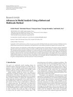
An example of sine BOC-modulated waveforms for N
BOC
= 1, 2, 3 is shown in Figure 1.Weremark,from(1), (2), and
(4), that N
BOC
= 1 corresponds to a BPSK-modulated PRN
sequence.
The normalized baseband power spectral density (PSD)
1
of a sine BOC-modulated signal is given in [4, 36, 37]:
X
BOC
( f )
=
⎧
⎪
⎪
⎪
⎪
⎪

⎪
⎨
⎪
⎪
⎪
⎪
⎪
⎪
⎩
1
T
c

sin

πfT
c
/N
BOC

sin

πfT
c

πf cos

πfT
c
/N

BOC


2
, N
BOC
even,
1
T
c

sin

πfT
c
/N
BOC

cos

πfT
c

πf cos

πfT
c
/N
BOC



2
, N
BOC
odd.
(5)
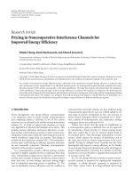
An example of the PSD for several BOC-modulated signals
(with N
BOC
from 1 to 4) is shown in Figure 2. The situa-
tion with N
BOC
= 1 coincides with BPSK modulation (e.g.,
such as for GPS C/A code). The even-modulation orders en-
sure a splitting of the spectrum into two symmetrical parts,
by moving the energy of the signal away from the DC fre-
quency, and therefore allowing for less interference in the
1
ThenormalizationwasdonewithrespecttothechipintervalT
c
,or,
equivalently, to the signal power over infinite bandwidth, similar to [4].
4 EURASIP Journal on Applied Signal Processing
012345
Chips
−1
0
1
BOC-modulated
code

PRN sequence (N
BOC
= 1)
(a)
012345
Chips
−1
0
1
BOC-modulated
code
PRN sequence (N
BOC
= 2)
(b)
012345
Chips
−1
0
1
BOC-modulated
code
PRN sequence (N
BOC
= 3)
(c)
Figure 1: Examples of time-domain waveforms for BOC-modulat-
ed signals.
existing GPS bands. The most representative case is that
one for N

BOC
= 2, which corresponds to the currently se-
lected modulation format by the Galileo Signal Task Force
(i.e., sine BOC(1, 1)). The cases with odd modulation index
(e.g., N
BOC
= 3) do not suppress completely the interference
around the DC frequency.
The baseband model of the received signal after the fad-
ing channel can be w ritten as
r(t)
=

E
b
e
+ j2πf
D
t
L

l=1
α
n,l
(t)x
BOC
(t − τ
l
)+η(t), (6)
where E

b
is the bit or symbol energy of the signal (one symbol
here is equivalent with one code epoch, and it typically has a
duration of T
= 1ms), f
D
is the Doppler shift introduced
by the channel, L is the number of channel paths, α
l,n
(t)is
the time-varying complex fading coefficient of the lth path
during the nth code epoch, τ
l
is the corresponding path de-
lay (assumed to be constant during the observation inter-
val), and η(
·) is an additive noise component of double-sided
wideband power spectral density N
w
, which incorporates the
additive white noise of the channel and the interference com-
ing from the other satellites. We remark that the relationship
between the bit energy-to-noise ratio E
b
/N
w
(in dB) and the
−15 −10 −50 51015
Frequency (MHz)
−80

−70
−60
−50
−40
−30
−20
PSD (dB-Hz)
N
BOC
= 1(BPSK)
N
BOC
= 2 (e.g., BOC(1, 1))
N
BOC
= 3 (e.g., BOC(15, 10))
N
BOC
= 4 (e.g., BOC(10, 5))
Figure 2: Examples of baseband PSD for BOC-modulated signals,
f
c
= 10.23 MHz.
carrier-to-noise ratio (CNR, in dB-Hz) is [39]
E
b
N
w
[dB] = CNR [dB-Hz] + 10log
10


T
c

. (7)
The acquisition and tracking of the received signal are
based on the correlation with the reference PRN code with
different time lags τ and frequency shifts f . After the data
modulation removal,
2
the correlation with the reference
PRN code, and the coherent integration over N
c
T seconds
at the receiver (N
c
is the coherent integration time in code
epochs or in ms if T
= 1 ms), we can obtain, after straightfor-
ward computations, a two-dimensional time-frequency ma-
trix R with elements R( f , τ) as follows:
R( f ,τ)
=

E
b
e
jπ( f
D
− f )N

c
T
sinc

π

f
D
− f

N
c
T

×
L

l=1
α
l
R
BOC

τ − τ
l

+ η( f , t),
(8)
where sinc(x)  sin(x)/x and the subscript n has been
dropped for simplicity. Above, the filtered noise

η(·) incor-
porates the intersymbol interference as well. By virtue of cen-
tral limit theorem, we assume that
η(·) is a zero-mean Gaus-
sian noise process. The notation
α
l
stands for the averaged
channel coefficients over N
c
code epochs. Clearly, if the co-
herent integration time is higher than the coherence time of
the channel, the received signal will be severely distorted. The
2
Here, we assume either that the data bits have been previously estimated
and removed from the received signal, or that a pilot signal is available.
Errors in data bit estimates are not analyzed here, but may deteriorate the
performance of the algorithms.
ElenaSimonaLohanetal. 5
−1 −0.500.51
Chips
−1
−0.5
0
0.5
1
Normalized ACF
Ideal ACF for BOC-modulated signals
N
BOC

= 1(BPSK)
N
BOC
= 2 (e.g., BOC(1, 1))
N
BOC
= 3 (e.g., BOC(15, 10))
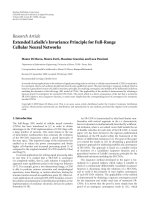
Figure 3: Examples of the real part of the ACF for BOC-modulated
signals.
term sinc(π( f
D
− f )N
c
T)in(8) is modeling the deterioration
due to a frequency error f
D
− f .In(8) R
BOC
(·) is the ideal
ACF of a sine BOC-modulated PRN sequence, given by (di-
rect consequence of (1)and(2), after several manipulations)
R
BOC
(τ) =
N
BOC
−1

i=0
N

BOC
−1

j=0
(−1)
i+ j
Λ
BOC

τ − (i − j)T
BOC

,
(9)
and Λ
BOC
(·) is the triangular-shaped ACF of an ideal PRN
sequence of period T
BOC
= T
c
/N
BOC
:
Λ(τ)
=
⎧
⎪
⎪
⎨

⎪
⎪
⎩
1 −|τ|
T
BOC
if |τ|≤T
BOC
,
0 otherwise.
(10)
Some examples of the real part of the ideal ACF of BOC-
modulated PRN sequences a re shown in Figure 3.
The two-dimensional matrix R with elements given in (8)
can be further noncoherently averaged over N
nc
blocks (i.e.,
the total coherent and noncoherent integration time will be
N
c
N
nc
T seconds). The noncoherent averaging may be needed
for further noise reduction, because the coherent averaging
interval is limited by the coherence time of the fading chan-
nel, by the stability of the local oscillator and by the possible
residual Doppler shift errors. However, there are some squar-
ing losses in the signal power due to noncoherent averaging.
Examples of coherence times (Δt)
coh

of Galileo channels for
a carrier frequency of f
carrier
= 1.575 GHz (corresponding
to E2-L1-E1 band [2]) are given in Tabl e 1 , according to the
definition in [40], namely, (Δt)
coh
≈ c/v f
carrier
,wherev is the
ground receiver speed and c is the speed of light. We remark
that the coherent integration time should be less than the val-
ues given in Table 1 , in order to keep the fading spect rum
Table 1: Channel coherence times for various receiver speeds for
Galileo E2-L1-E1 signal.
Speed
2 4 20 40 80 120
(km/h)
Coherence
342.8 171.42 34.28 17.14 8.57 5.71
time (ms)
500
0
−500
Frequency error (Hz)
0
2
4
6
8

10
Time window (chips)
0
1
2
3
4
5
6
×10
−2
Average time-frequency
correlation
CNR = 34 (dB-Hz), N
c
= 30 ms, N
nc
= 10 blocks, L = 6paths
Figure 4: Examples of the time-frequency correlation (or matched
filter) mesh after coherent and non-coherent integration, 6 closely
spaced paths.
of the signal undistorted. Tabl e 1 takes into a ccount only the
receiver ground speed. We remark that there is also a rela-
tive speed of the mobile receiver with respect to the satellite
speed, which is much higher than the receiver ground speed.
This will create a Doppler shift effect on the signal (as seen in
(6)). Thus, we have both a Doppler shift (due to the satellite
movement) and a Doppler spread around the Doppler shift
frequency (due to the receiver movement). The Doppler shift
should be estimated and removed before the coherent inte-

gration ( we assume that this has been done in the acquisition
stage). If there remains some residual Doppler errors, then
the values given in Tabl e 1 become very loose upp er bounds
on the coherent integration times.
The delay estimation is done on a time-frequency grid
whose values are the averaged correlation functions with dif-
ferent time and frequency lags. As seen in (8), the maxima
occur at f
= f
D
and τ = τ
l
. An example of a time-frequency
grid for a 6-path Rayleigh fading channel, covering a fre-
quency offset of 1 kHz and a time window of 10 chips, is
shown in Figure 4.
3. DELAY ESTIMATION ALGORITHMS
3.1. Feedback estimators
Traditionally, the multipath delay estimation block is imple-
mented via a feedback loop. The most common feedback
6 EURASIP Journal on Applied Signal Processing
−1 −0.500.51
Delay error (chips)
−1.5
−1
−0.5
0
0.5
1
1.5

2
2.5
3
S-curve
Ideal S-curve, noncoherent narrow correlator,
Δ
E−L
= 0.1 chips
N
BOC
= 1(BPSK)
N
BOC
= 2 (e.g., BOC(1, 1))
N
BOC
= 3(e.g.,BOC(1.5, 1))
Figure 5: Ideal S-curve for BPSK and sine BOC modulations,
Δ
E−L
= 0.1 chips.
structures for the delay estimation are the so-called DLLs
[3, 5, 13, 17, 20]. Several enhanced DLLs have been pro-
posed in the presence of multipaths. One example is the
narrow correlator [22–24], where the spacing Δ
E−L
between
early and late correlators is reduced below 1 chip. The perfor-
mance of narrow correlator is somehow limited in closely-
spaced multipath scenarios [23]. Another example is the

Rake DLL (RDLL) [21, 28]whichusesaseparatemulti-
path channel estimation unit which provides the estimates
of the interfering path parameters. The estimated parame-
ters are used in a Rake-like structure to resolve and combine
the received multipath components. The RDLL is concep-
tually close to the DLL with interference-cancellation (IC)
[13, 17]. The DLL with IC subtrac ts the estimated contribu-
tion of interfering paths from the output of the finger track-
ing the path of interest. Another improved variant of DLL is
the so-called DLL with interference-minimization (IM) tech-
nique [13]. The idea of the DLL with IM is to filter the out-
puts of the correlators with some adaptive filter, whose co-
efficients are designed in such a way to minimize the mul-
tipath interference. Similar ideas can be found also in the
Phase Multipath Mitigation Window Correlator (PMMWC),
proposed in [41]. Again, the knowledge about the interfering
path parameters should be obtained via an additional multi-
path channel estimation unit. Since RDLLs, PMMWCs, DLLs
with IC and DLLs with IM are conceptually close, we illus-
trate here the performance of a DLL with IC in the presence
of multipaths and BOC modulation.
The perfor m ance of the DLL is best illustrated by the so-
called S-curve, which presents the expected value of the error
signal as a function of the reference parameter error (i.e., the
code phase error) [6]. Figure 5 shows the S-curve in single-
path channel for BPSK and two BOC-modulated signals. The
−1 −0.500.51
Delay error (chips)
−1.5
−1

−0.5
0
0.5
1
1.5
2
2.5
3
S-curve
S-curve for BOC-modulation, N
BOC
= 2, and 4
closely spaced paths
Global S-curve, no interference cancellation (IC)
S-curve of first path with IC, no channel estimation errors
S-curve of first path with IC and small channel estimation
errors (i.e., 0.05 delay error and 0.01 amplitude error)
True path delays (with respect to LOS)
Figure 6: Performance of a DLL with IC in the presence of multi-
path channels and BOC modulation (N
BOC
= 2), Δ
E−L
= 0.1 chips,
channel path delays at [0, 0.04, 0.07, 0.1] T
c
, channel path ampli-
tudes [0.8, 1, 0.7, 0.4].
number of side-lobes increases as the BOC modulation order
N

BOC
increases. The zero-crossings from b elow here indicate
the presence of a multipath. However, for BOC-modulated
signals, the search range should be decreased to less than
2 chips (as it is the case for BPSK modulation). For example,
as seen in Figure 5,forN
BOC
= 2 (e.g., BOC(1, 1)), the search
range should be between
−1/(2N
BOC
)and+1/(2N
BOC
) chips,
in order to have convergence and to avoid the false lock
points. In order to cope with the side-lobes of the ACF func-
tion, a very early-very late (VE-VL) loop with a narrower
correlator spacing was proposed for Galileo and modern-
ized GPS signals [3]. The typical DLLs have early, late, and
prompt correlators to track the delays. The VE-VL loops in-
troduce two extra correlators (one very early, another one
very late) in order to check better that the prompt reference
signal is aligned with the main peak of the correlation func-
tion, and not a secondary peak. Conceptually, a very early-
very late DLL is close to the sample-correlate-choose largest
(SCCL) algorithm [19] and, to some extent, also to the high
resolution correlator (HRC) [24]. However, in VE-VL case,
the additional correlators are used only to check that the
main peak is on the prompt, but they are not used directly
in the tracking [3], while in HRC case, an S-curve is formed

based on the 4 correlators (early, late, very-early, and very-
late) and the delay is tracked according to this S-curve [24].
If multipath components are present, the performance of
an enhanced DLL is shown in Figure 6 (here, a coherent DLL
with IC is selected for illustration purpose). The channel has
ElenaSimonaLohanetal. 7
4 in-phase static paths, and the first path is weaker than the
second one (see Figure 6 caption). In the absence of any IC,
the channel paths are merging (here, we showed the situa-
tion of closely spaced paths) and the S-curve is not able to
track correctly the LOS delay. In the presence of IC, if the
multipath channel estimation unit operates perfectly (i.e., no
channel estimation errors), the DLL with IC is able to track
correctly the LOS component (see Figure 6). However, even
small channel estimation errors will destroy completely the
ability of the DLL to track the LOS correctly, as shown in
Figure 6. For example, the delay error for the narrow correla-
tor (no IC) was 0.05 chips (i.e., 14.66 m), and, for DLL with
IC and channel estimation errors, it becomes 0.09 chips (i.e.,
26.39 m).
To summarize the discussion about feedback tracking
loops (i.e., DLLs and their enhanced variants), the main
drawbacks of the DLL-based techniques include their re-
duced ability to deal with closely spaced path scenarios un-
der realistic assumptions (such as the presence of errors in
the channel estimation process), their relatively slow conver-
gence, the small pull-in range if small spacing (such as for
narrow correlator) is used, and the possibility to lose the lock
(i.e., start to estimate the delays with high estimation error)
due to the feedback error propagation. Moreover, the DLL-

based techniques work only under the assumption that the
initial delay error is sufficiently small (e.g., for BOC signals
smaller, in absolute value, than 1/(2N
BOC
) chips due to the
fades in the ACF, as seen in Figure 3).
Despite their disadvantages, the feedback DLL-based
approaches are still the tracking structures of choice for
nowadays receivers, due to a number of positive features.
Among the advantages of DLLs we have the fact that only
3 correlators are typically needed (or at most 5, e.g., for HRC
or VE-VL structures), DLLs behaves good in friendly envi-
ronments (e.g., distant paths, single path channels, etc.), and
there is no need of thresholding as in the case of feedforward
techniques (this will be explained in detail in Section 3.3).
It is the purpose of our paper to show that feedforward
delay estimation techniques may be, however, feasible alter-
natives to feedback tracking loops, in terms of good accuracy
of the delay estimation process and reasonable complexity, as
it will be shown in what follows. Due to the fact that feedback
tracking loops are based on the assumption that the acqui-
sition stage provide a sufficiently small error (otherwise the
loop will not converge to the correct path delay), it is hard
to make a per formance comparison between feedback and
feedforward techniques. The feedback techniques are meant
to keep the lock, that is, to keep the initial delay estimate as
accurate as possible, but once the lock is lost, the acquisition
process should be restarted. The feedforward techniques can
be seen as one-shot estimates,
3

which do not need very ac-
curate initial delay estimates in the tracking process (delay
errors of the order of chips or tens of chips are possible). For
these reasons, the measures of performance are rather dif-
3
When iterative estimates are needed, the same one-shot principle can be
applied, by using the previous delay estimates as the starting point when
defining the search window for the new delay estimates.
ferent in feedback and feedforward algorithms (i.e., for the
former, typical measures are the time-to-lose lock and the
code tracking noise standard deviation, while for the later,
the root-mean-square delay errors and detection probabili-
ties are typically used).
3.2. Feedforward estimators
The authors have previously proposed several feedforward
delay estimation techniques [9, 30, 32, 42, 43]asefficient al-
ternatives to the DLLs-based techniques. These feedforward
techniques have been extensively studied for WCDMA sig-
nals and BPSK modulation and, among them, the Teager-
Kaiser (TK) and the deconvolution-based (namely, projec-
tion onto convex sets POCS) algorithms proved to be the
most promising from the point of view of their performance
in closely spaced path scenarios. It is therefore of interest to
analyze the behavior of these algorithms in the presence of
BOC-modulated PRN codes as well. In what follows, we start
from the simplest feedforward estimator, namely, the corre-
lator or matched filter (MF) and then, we present the ideas
behind TK and deconvolution-based algorithms.
Based on (8), the MF output at a certain estimated Dop-
pler frequency


f
D
is
J
MF
(τ) = R


f
D
, τ

. (11)
The estimate of the Doppler frequency

f
D
is obtained as
the frequency corresponding to the global maximum of the
time-frequency mesh illustrated in Figure 4. We remark that,
for a fair comparison, the same

f
D
estimated (based on MF
output) is kept for all the compared delay estimators; only the
delay estimation process is different. By taking the discrete
samples τ
= lT

s
of the MF output of (11), we can rewrite the
MF output in a vectorial form [30] (needed to explain the
deconvolution algorithms):
J
MF
= G
BOC
h + v, (12)
where J
MF
= [J
MF
(d
min
T
s
), , J
MF
(d
max
T
s
)]
T
, d
min
is the
minimum delay in samples, and d
max

is the maximum delay
in samples (i.e., the time-window or the delay spread over
which we look for the channel paths spans between d
min
T
s
and d
max
T
s
seconds, and d
min
and d
max
are chosen as integer
multiples of the sampling period, for the sake of the simu-
lation model), the sampling interval T
s
is chosen sufficiently
small to model fractional path delays
4
(e.g., T
s
= 0.05T
BOC
).
We remark that, similarly with feedback techniques, d
min
and d
max

can be chosen in such a way to capture the channel
true delays, based on previous delay estimates or based on the
acquisition stage. For example, for diminishing the number
4
The fractional delays model and the estimation of the delays with high
accuracy can be achieved either via a sufficiently small sampling interval
(i.e., a high number of samples per chip), or, equivalently, via interpola-
tion. Interpolation-based algorithms may decrease the receiver complex-
ity and constitutes a topic of future research.
8 EURASIP Journal on Applied Signal Processing
of correlators required by the model, an initial acquisition
stage can take place (where a coarse delay estimate
τ
LOS
is formed), then the feedforward-based fine delay estima-
tion stage will perform the correlations only
±D
max
/2 chips
around
τ
LOS
,whereD
max
is the search window length in chips
(i.e., d
min
= (τ
LOS
− D

max
/2)N
s
N
BOC
and d
max
= (τ
LOS
+
D
max
/2)N
s
N
BOC
). For feedback tracking techniques, the LOS
delay is typically tracked within
±1 chip around the previous
delay estimate, while in our case, we can have D
max
> 2 chips
(indeed, in our simulation we used a D
max
between 4 and
10 chips).
Above, G
BOC
is the ideal autocorrelation matrix of size
N

× N (N = d
max
− d
min
), including the effect of BOC
modulation and having the elements g(i, j)
= R
BOC
((i −
j)T
s
), i, j = 1, , N,andh is a N × 1 vector, includ-
ing the channel effect and having the ith element equal to

E
b
e
jπΔ f
D
N
c
T
sinc(πΔ f
D
N
c
T)h
i
, i = d
min

, , d
max
, Δ f
D
=
f
D
−

f
D
,and
h
i
=
⎧
⎨
⎩

α
i
if a channel path is present at the time delay iT
s
,
0 otherwise.
(13)
The term v is the noise vector, with the elements
η(

f

D
, iT
s
)
(including various noise sources such as the background
noise, the nonidealities of the PRN code sequences, the pos-
sible interference between two or more satellites, etc.), i
=
d
min
, , d
max
. The MF estimate of the squared channel coef-
ficient envelope
|h|
2
is given by the noncoherently averaged
MF output:

h
MF
=
1
N
nc
N
nc

1
|J

MF
|
2
, (14)
where N
nc
is the noncoherent integration time. In what fol-
lows,wewillreferto

h estimates also as “cost functions.” Sim-
ulation results showed that using the squaring-absolute value
operator (instead of the absolute value itself) gives slightly
better results. The noncoherent squaring losses are indeed
present, but noncoherent averaging might still be needed,
due to the limits in the coherent integration (e.g., residual
Doppler shifts, instabilities of oscillator clock, etc.)
Resolving the multipath components can be seen as a de-
convolution problem [30] in which we try to estimate the
nonzero elements of the unknown gain vector h. The first
nonzero component higher than a threshold will be the esti-
mate of the first arriving path.
The well-known least squares (LS) solution is given by
[9]

h
LS
=

G
H

BOC
G
BOC

−1
G
H
BOC

h
MF
. (15)
We remark that the above LS solutions also suffer of non-
coherent losses, due to the fact that we use

h
MF
in the estima-
tor, instead of J
MF
. Thus, the noise statistics are modified (to
a chi-square distribution), and the LS solution becomes sub-
optimal. However, due the practical limits of coherent inte-
gration mentioned above, the noncoherent squaring should
be usually employed. Indeed, simulation results w ith even a
small residual Doppler shifts showed that, by using coherent
integration alone, we cannot achieve satisfactory results. The
solution given by (15) is known to be very sensitive to noise
and often the matrix G
H

BOC
G
BOC
is ill-conditioned. It w ill be
kept in what follows as a reference, but the results will be
shown to be very poor, as expected. More robustness to the
noise is given by the so-called minimum mean square error
(MMSE) solution, given by

h
MMSE
= (σ
2
I + G
H
BOC
G
BOC
)
−1
G
H
BOC

h
MF
, (16)
where I is the unity matrix and
σ
2

is the estimate of the noise
variance, obtained directly from the MF output

h
MF
,asitwill
be discussed in Section 3.3.
In order to cope with the noise in even a better way and
in order to solve the problem of closely spaced paths, the
MMSE solution can be developed into a constrained itera-
tive deconvolution technique, called projection onto convex
sets (POCS), which was introduced in [33, 44], for the Rake
receiver with rectangular pulse shapes, and later applied for
WCDMA signals [9, 30]. The POCS algorithm is an itera-
tive method that finds a feasible solution consistent with a
number of constraints [12]. Starting with an initial guess of
the solution, the algorithm converges to a feasible solution
by cyclically projecting into constraint sets. Thus, POCS es-
timator of h has the form

h
POCS
= P
C
h,whereP
C
(·) is the
projection operator and C is the convex set defined by the MF
output: C
={f, J

MF
− G
BOC
f
2
≤ ξ} [33, 44]where·is
the L2 vector norm (i.e., by definition, if z is a column vec-
tor, its L2normis
z
2
= z
h
z), and ξ is a scalar bound, given
by the variance of the noise at the output of MF. The POCS
solution is found by solving the following quadratic program
[43]:
⎧
⎪
⎨
⎪
⎩
min

h
POCS



h
POCS

−|h|
2


2
,
under the constraint:


J
MF
− G
BOC
h


2
≤ ξ
⎫
⎪
⎬
⎪
⎭
. (17)
The squaring of the channel vector h in the above equa-
tion was necessary because the

h estimates given here (for all
the algorithms) are, in fact, the estimates of
|h|

2
(and not of
the channel coefficient vector h). This fact does not have any
impact on the delay estimates, since we are not interested in
the exact values of the channel coefficients, but only on their
relative magnitudes (i.e., we are interested in finding those
values of estimated vectors

h which are higher than a certain
threshold).
The above quadratic program can be solved iteratively
and POCS estimation can take place in several stages. At stage
k + 1, the POCS estimate can be w ritten as [12, 30, 43]

h
(k+1)
POCS
=

h
(k)
POCS
+

1
λ
I + G
H
BOC
G

BOC

−1
× G
H
BOC


h
MF
− G
BOC

h
(k)
POCS

,
(18)
ElenaSimonaLohanetal. 9
−1.5 −1 −0.500.511.5
Delay error (chips)
0
0.2
0.4
0.6
0.8
1
1.2
Cost functions

Ideal ACF of sine BOC(1, 1) (envelope)
TK applied on squared ideal envelope
Figure 7: Illustration of TK applied on the squared envelope of an
ideal ACF of sine BOC(1, 1) signal (no noise).
where λ is a constant determining the convergence speed (it
also represents the Lagrange multiplier associated with the
constraint of (17)). The initial estimate for

h
POCS
is the MF
estimate:

h
(1)
POCS
=

h
MF
. The final cost function for POCS es-
timation is

h
POCS
=

h
(N
iter

)
POCS
.
In practice, iterations are performed until no significant
improvement from iteration to iteration is achieved. Opti-
mally, λ should be adjusted based on the noise variance and
the other bounds in the optimization process [12, 14, 45];
however, this adjustment is a laborious process, based on a
priori knowledge of noise statistics (which, in practice, might
be unknown). Moreover, the simulation results w ith var ious
λ values between 0.01 and 10 showed us that the variation of
λ does not have a significant impact on the delay estimation
accuracy and that choosing λ
∈ [0.1, 1] slightly outperforms
the cases when λ>1 (thus, λ
= 0.5 is a reasonable choice).
Also based on simulations, we noticed that we need at least
N
iter
= 10 iterations in order to be able to separate the closely
spaced paths, which is also in accordance with the results re-
ported in [14].
We remark that the notion of closely spaced paths refers
usually to paths separated at less than one chip interval [7, 9–
16]. However, due to the narrower width of the main lobe
of the ACF in the presence of BOC modulation (as seen in
Figure 3), the most challenging cases will be in fac t those with
a path separation of less than 1/(N
BOC
) chips, as it will be

seen from the simulation results.
The nonlinear quadratic TK operator was first intro-
duced for measuring the real physical energy of a system [46].
Since its introduction, it has widely been used in various
speech processing and image processing applications and,
more recently, it has also been applied in CDMA applications
[9, 30, 34, 35 , 42]. The discrete-time TK operator Ψ
d
(·)ofa
complex-valued discrete signal z(n)is[9, 42]
Ψ
d

z(n)

 z
2
(n − 1) −
1
2

z(n − 2)z
∗
(n)+z(n)z
∗
(n − 2)

,
(19)
and the discrete-time TK operator Ψ

d
(·)ofareal-valueddis-
crete signal z(n)becomes
Ψ
d

z(n)

 z(n − 1)z
∗
(n − 1) − z(n − 2)z(n). (20)
In our case, TK operator is applied on the squared-absolute
value of the MF output, and the cost function for TK algo-
rithm (after noncoherent averaging) is

h
TK
=



Ψ
d




h
MF



2




. (21)
The reason for choosing TK operator in the algorithm com-
parison is its good performance reported in multipath sce-
narios for WCDMA systems [9, 30, 42]. We remark that TK
operator was first applied at different levels of the corre-
lation function: before coherent integration, before nonco-
herent integration, and after both coherent and noncoher-
ent integration. The results showed that the best results are
obtained when TK is applied after noncoherent integration
(and therefore, on the squared-absolute value of the averaged
correlation function), as shown in (21), and the results are
only shown for this case. For the other situations (i.e., TK
applied before integration), the results are quite poor, due
to the high noise levels and to the sensitivity of TK opera-
tor to the noise. The intuitive behavior of TK algorithm is
illustrated via Figure 7, where we show the envelope of a sine
BOC(1, 1) signal (continuous line) together with the output
of TK operator applied on the squared envelope of the ACF.
We notice that TK is able to distinguish the global peak (cor-
responding to the zero delay error) among the spurious side-
lobes of the sine-BOC ACF. The side-lobes are not completely
cancelled out after applying TK operator, but their levels are
much diminished after TK. This property of TK to preserve
only the useful energy of the correlation function will b e in-

deed beneficial for closely spaced channel paths (see later on
the explanations with respect to Figure 9).
In Figures 8 and 9 we illust rate the per formance of POCS
and TK, respectively, in the presence of 4 closely spaced paths
and BOC-modulated PRN codes (the noiseless case is shown
here). A scenario with LOS path weaker than a successive
NLOS component was selected for illustrative purposes. The
same channel profile as that one used for Figure 6 is also used
here. Typically, better results are achieved when LOS path
is the strongest one. The true channel path delays are plot-
ted with their respective magnitudes for reference purposes.
From the matched filter output, we cannot distinguish the
presence of multipath components. If the estimation is based
on MF output, the delay estimation error would be 0.05 chips
(which translates into about 14.6 m distance error for a chip
rate of 1.023 MHz). By applying TK operator (Figure 9), all
the four channel paths are easily distinguished. POCS esti-
mates (Figure 8) are a little bit noisier, but they are still es-
timating the LOS delay better than MF ( in this example, the
delay error for the first path is 0.02 chips or 5.86 m).
10 EURASIP Journal on Applied Signal Processing
0.511.52
Channel delays (chips)
0
0.2
0.4
0.6
0.8
1
ACF and POCS

MF output
POCS output
True channel paths
Illustration of POCS principle, multipath static channel,
no noise
Figure 8: Illustration of POCS delay estimation algorithm in the
presence of BOC(2, 2) or BOC(1, 1) modulation (N
BOC
= 2) and 4
closely spaced paths.
3.3. Threshold setting
As explained above, a threshold is necessary to be set in or-
der to select the first significant local maximum of the cost
function

h (e.g.,

h
MF
,

h
TK
,

h
POCS
, etc.). The time position of
the channel paths is determined as the position of the local
peaks of the cost function w hich are higher than a threshold

γ. This threshold was built based on the ideal ACF of BOC-
modulated signal together with the estimate of the noise vari-
ance:
γ
= γ
1
+

σ
2
, (22)
where γ
1
is the second highest peak of an ideal ACF in
the presence of BOC modulation (e.g., as seen in Figure 7,
γ
1
= 0.5forN
BOC
= 2), and σ
2
is the estimate of the noise
variance, obtained directly from the cost func tion

h
alg
as the
mean of the squares of out-of-peak values of

h

alg
. An out-of-
peak (OOP) value is a value which is at least one chip apart
from the global peak and alg stands for one of the MF, LS,
MMSE, POCS, or TK algorithms:
σ
2
=
1
N
OOP

n∈indices of OOP values



h
alg
(n)


2
. (23)
Above, N
OOP
is the number of discrete OOP samples and

h
alg
(n) are the elements of the


h
alg
vectors. Equation (22)has
been used for MF, POCS, MMSE, and LS estimates. For TK
algorithm, γ
1
is obtained directly from the TK applied on the
square envelope of an ideal ACF (see Figure 7), and the noise
variance is obtained directly from the MF output. An exam-
ple for the threshold computation for MF and TK outputs is
0.511.52
Channel delays (chips)
0
0.2
0.4
0.6
0.8
1
ACF and TK
MF output
TK output
True channel paths
Illustration of TK principle, multipath static channel,
no noise
Figure 9: Illustration of TK delay estimation algorithm in the pres-
enceofBOC(2,2)orBOC(1,1)modulation(N
BOC
= 2) and 4
closely spaced paths.

shown in Figure 10 for a 4-path fading channel and CNR of
27 dB-Hz. The true LOS delay and the estimated LOS delay
are also written in each plot.
We also remark here that the side-lobes of a sine BOC-
modulated signal appear at the delays τ
sidelobes
,givenby
τ
sidelobes
= arg max
τ
R
BOC
(τ), (24)
with R
BOC
(τ)givenin(9). For example, the side peaks for
sine BOC(1, 1) modulation (N
BOC
= 2) occur at ±0.5 chips
around the global maximum, for sine BOC(15, 10) (N
BOC
=
3) occur at ±0.33 and ±0.67 chips, and for sine BOC(10, 5)
(N
BOC
= 4) occur at ±0.25, ±0.5, and ±0.75 chips. Gener-
ally, there are 2N
BOC
−2 side-lobes in the correlation function

which interfere with the channel paths and may create false
lock points. However, the most significant ones are those
with the smallest delay relative to the global maximum. This
is the reason for which the threshold estimation is based on
the second highest peak of the ideal ACF given in (9).
4. PERFORMANCE COMPARISON
In what follows, the perfor mance of the discussed feedfor-
ward delay estimation algorithms is compared in terms of de-
tection probability P
d
and root-mean-square error (RMSE).
The reason for not including the feedback delay estimation
algorithms in this comparison is that there is no possibil-
ity of a fair comparison between the two. This comes from
the fact that the performance measure for feedback-based
algorithms is typically the time-to-lose lock, which has no
equivalent for the feedforward-based algorithms. Moreover,
ElenaSimonaLohanetal. 11
3.23.33.43.53.63.73.8
Channel delays (chips)
0
0.1
0.2
0.3
0.4
0.5
0.6
0.7
0.8
0.9

1
h
MF
MF output
True channel paths
Estimated threshold
Tru e LOS
= 3.3878 chips
Estimated LOS
= 3.45 chips
(a) Estimated threshold: γ = 0.53763
3.23.33.43.53.63.73.8
Channel delays (chips)
0
0.1
0.2
0.3
0.4
0.5
0.6
0.7
0.8
0.9
1
h
TK
TK output
True channel paths
Estimated threshold
Tru e LOS

= 3.3878 chips
Estimated LOS
= 3.4 chips
(b) Estimated threshold: γ = 0.37032
Figure 10: MF and TK outputs (main lobe) for a 4-path fading
channel and the estimation of the threshold, N
BOC
= 2, CNR =
27 dB-Hz, N
c
= 180, N
nc
= 8.
in feedback-based algorithms, we have to assume that the ini-
tial delay error is less than 1/(2N
BOC
) c hips in order for the
algorithm to converge (which is a very restrictive assump-
tion).
The performance of the algor ithms for channel profiles
has been analyzed and the most representative results have
been included. Two main channel profiles have been consid-
ered (both may be seen as typical indoor channels, due to
large number of closely spaced paths and low mobile speeds):
Table 2: Parameters of the simulations.
N
BOC
BOC modulation order
N
c

Coherent integration time (ms)
N
nc
Noncoherent integration time
(blocks of N
c
ms)
v Mobile receiver speed (km/h)
x
max
Maximum separation between successive
paths (chips)
α Vector of average path powers (dB)
L Number of channel paths (if constant)
L
max
Maximum number of channel paths
(if random)
μ
PDP
Exponential factor for the decaying
PDP model (chips
−1
)
Δε
P
d
The error for which the detection probability
is computed (chips), that is, detection is done
within

−Δε
P
d
to +Δε
P
d
chips error
(i) indoor with Rayleigh distribution of all paths, decay-
ing power delay profile (PDP) and a random number
of paths, uniformly distributed between 1 and L
max
=
7,
(ii) indoor with fixed Rayleigh PDP (first path having a
smaller average power than the second one) and L
= 4
paths.
The mobile speed was set to v
= 4 km/h (we remark that
simulations with higher mobile speeds and with Rician fad-
ing profiles have also been performed and similar conclu-
sions were drawn). The channel models used here are based
on some typical fading channel models reported in the liter-
ature [9, 40, 47]. A main parameter of the channel model is
the separation between successive paths, which was assumed
to be uniformly distributed between 0 and x
max
(where x
max
is the maximum separation between successive paths).

When the decaying PDP is used, the average path power
α
l
of the lth path is given according to its distance from the
first arriving path and to an exponential factor μ
PDP
in the
form
α
l
= α
1
e
μ
PDP
(τ
l
−τ
1
)
.
The detection probability P
d
is defined as the probabil-
ity to detect the first arriving path (hereby assumed to be
LOS path) with an absolute error smaller than or equal to
Δε
P
d
. The LOS delay estimation is done only at the correct

frequency bin (with a possible small residual Doppler error,
smaller than 1/N
c
KHz), and with a time-window D
max
,as
seen in Section 3.2. The main parameters of the simulation
model are summarized in Ta ble 2 and their values are given
in the caption of each figure.
The comparison between the MF, TK, POCS, and LS al-
gorithms for various channel profiles is shown in Figures 11
and 12 (the plots versus CNR), in Figure 14 (the plots ver-
sus N
BOC
), and in Figure 15 (the plots versus N
c
). Clearly, LS
algorithm fails to work properly due to the noise enhance-
ment property specific to LS approaches. MMSE algorithms
12 EURASIP Journal on Applied Signal Processing
15 20 25 30 35
CNR (dB-Hz)
0
0.1
0.2
0.3
0.4
0.5
0.6
0.7

0.8
0.9
Detection probability within 0.025 chips
MF
TK
POCS
MMSE
LS
(a) Indoor channel, decaying PDP, x
max
= 0.1 chips, L
max
= 7
paths
15 20 25 30 35
CNR (dB-Hz)
10
−2
10
−1
10
0
10
1
RMSE (chips)
MF
TK
POCS
MMSE
LS

(b) Indoor channel, decaying PDP, x
max
= 0.1 chips, L
max
= 7paths
Figure 11: Comparison of feedforward delay estimation algorithms
as a function of CNR, indoor channel, decaying PDP, μ
PDP
= 0.5,
x
max
= 0.1 chips, N
c
= 180, N
nc
= 8, N
BOC
= 2, L
max
= 7 paths,
v
= 4km/h. P
d
within Δε
P
d
= 0.025 chips error (a) and RMSE in
chips (b).
is better than LS, but it is still surpassed by TK and POCS,
and, in some cases, even by MF; one reason might be the fact

that MMSE is using the estimated noise variance, and not
the true noise variance (which is hard to get in practice), and
therefore, it mig ht be affected by the errors in this estimate.
We noticed from Figures 11 and 12 that MF algorithm
is not able to distinguish well between very closely spaced
15 20 25
30
35
CNR (dB-Hz)
0
0.1
0.2
0.3
0.4
0.5
0.6
0.7
Detection probability within 0.025 chips
MF
TK
POCS
MMSE
LS
(a) Indoor channel, fixed PDP, x
max
= 0.2 chips, L = 4paths
16 18 20 22 24 26 28 30 32 34
CNR (dB-Hz)
10
−1

10
0
RMSE (chips)
MF
TK
POCS
MMSE
LS
(b) Indoor channel, fixed PDP, x
max
= 0.2 chips, L = 4paths
Figure 12: Comparison of feedforward delay estimation al-
gorithms as a function of CNR, indoor channel, fixed PDP:
α =[−2, 0, −1, −4] dB, x
max
= 0.2 chips, L = 4 paths, N
c
= 180,
N
nc
= 8, N
BOC
= 2, v = 4km/h.P
d
within Δε
P
d
= 0.025 chips error
(a) and RMSE in chips (b).
paths (i.e., maximum spacing less than 0.2 chips), and there-

fore, it suffers from a saturation effect at higher CNRs (see
the P
d
curves in the above-mentioned plots). Both TK and
POCS have much better detection probability than MF algo-
rithms if the CNR is sufficiently high (or, equivalently, if we
use enough integration to smooth the signal). This is due to
the fact that TK and PO CS can separate closely spaced paths,
ElenaSimonaLohanetal. 13
−0.6 −0.4 −0.200.20.4
Delay error (chips)
0
0.1
0.2
0.3
0.4
0.5
0.6
0.7
0.8
0.9
PDF
MF
TK
POCS
Figure 13: Distribution of delay estimation errors, indoor channel,
decaying PDP, μ
PDP
= 0.5, x
max

= 0.1 chips, N
c
= 180, N
nc
= 8,
N
BOC
= 2, L
max
= 7 paths, v = 4 km/h, CNR = 30 dB-Hz.
while the MF will always detect the merged peak, as shown
in Figures 9, 8,and10.
On the other hand, from the point of the RMSE value,
MF is not much worse than TK and POCS at high CNR v al-
ues and it is always better in severe noise conditions (low
CNR). This means that, when the estimate is noisy in TK
and POCS cases, this estimate is more likely to be an out-
lier, while for MF, it mostly remains in a neighborh ood of
the true path delays, but without being able to separate them.
The apparent contradiction between a good P
d
and a rather
poor RMSE is illustrated in Figure 13 via the probability dis-
tribution function (PDF) of the delay errors. This plot cor-
responds to the CNR
= 30 dB-Hz from Figure 11,wherewe
notice that P
d
of TK and POCS is much better than the P
d

of
MF, while the gap between the RMSE of TK and the RMSE
of MF is not very high, and POCS has even worse RMSE per-
formance than MF. If we look at the PDF of Figure 13,wesee
that MF estimate has a higher bias than the other two esti-
mates (due to the incapacity of MF to separate closely spaced
paths), but it also has less outliers.
We remark that, when we loosen the condition for the
allowed delay error Δε
P
d
(i.e., Δε
P
d
increases), the detec-
tion probability becomes better, as expected, but the general
shapes of the curves are preserved.
As seen in Figures 11 and 12, the behavior of the com-
pared algorithms is pretty similar in decaying PDP channels,
as well as in fixed PDP channels. However, if the first arriv-
ing path is weaker than the next arriving path, as in Figure 12,
the detection probability decreases for all the algorithms, and
MF is clearly not good enough to detect the first arriving peak
(neither in detection probability nor in RMSE).
From the comparison between different algorithms in
various channel profiles, we noticed that TK and POCS es-
11.522.533.54
N
BOC
0

0.1
0.2
0.3
0.4
0.5
0.6
0.7
0.8
0.9
1
Detection probability within 0.025 chips
MF
TK
POCS
MMSE
LS
(a) Indoor channel, decaying PDP, x
max
= 0.05 chips, L
max
= 7
paths
11.522.533.54
N
BOC
10
−2
10
−1
10

0
10
1
RMSE (chips)
MF
TK
POCS
MMSE
LS
(b) Indoor channel, decaying PDP, x
max
= 0.05 chips, L
max
= 7
paths
Figure 14: Comparison of feedforward delay estimation algorithms
as a function of N
BOC
, indoor channel, decaying PDP, x
max
=
0.05 chips, N
c
= 180, N
nc
= 8, CNR = 30 dB-Hz, v = 4km/h.
P
d
within Δε
P

d
= 0.025 chips error (a) and RMSE in chips (b).
timators are less robust to noise than MF estimator. This is
partial ly also due to the threshold computation γ,whichis
quite noisy in low CNR conditions, and therefore increases
the likelihood of picking a wrong local peak of the corre-
lation function as the LOS estimate. On the other hand, if
CNR after integra tion is sufficiently high, we notice that TK
and POCS offer the best separation between closely spaced
14 EURASIP Journal on Applied Signal Processing
50 100 150 200 250 300
N
c
(code epochs)
0
0.1
0.2
0.3
0.4
0.5
0.6
0.7
Detection probability within 0.025 chips
MF
TK
POCS
MMSE
LS
(a) Indoor channel, decaying PDP, x
max

= 0.1 chips, L
max
= 7
paths
50 100 150 200 250 300
N
c
(code epochs)
10
−2
10
−1
10
0
10
1
RMSE error (chips)
MF
TK
POCS
MMSE
LS
(b) Indoor channel, decaying PDP, x
max
= 0.1 chips, L
max
= 7paths
Figure 15: Comparison of feedforward delay estimation algorithms
as a function of N
c

, indoor channel, decaying PDP, x
max
= 0.1 chips,
N
nc
= 8, CNR = 22 dB-Hz, N
BOC
= 2, v = 4km/h. P
d
within
Δε
P
d
= 0.025 chips error (a) and RMSE in chips (b).
paths (i.e., they typically have the best detection probabilities
compared to the other algorithms).
Figure 14 shows the impact of the increasing N
BOC
,for
the indoor s cenarios with maximum path spacing x
max
=
0.05 chips (i.e., very closely spaced paths). Similar results
have been obtained for spacings up to x
max
= 0.2 chips. For
a fair comparison between the algorithms, we assumed that
the same target Δε
P
d

is aimed (here 0.025 chips). For MMSE
and LS, the P
d
performance is deteriorating when N
BOC
in-
creases (this is partially due to the errors in the noise variance
σ
2
estimation). For TK and POCS, the best P
d
performance is
achieved at N
BOC
= 2, while for MF the best P
d
is achieved at
N
BOC
= 3. This behavior is mainly due to the increase in the
number and amplitude of side-lobes in the ACF, when N
BOC
increases, a nd to the computation of the threshold, which is
sensitive to the height of the side-lobes. By optimizing the
choice of the threshold for each modulation order, the au-
thors believe that the performance at higher N
BOC
of all the
discussed algorithms can be improved. The side-lobes of the
ACF act as interferers in the estimation process, and it may

happen that the delay estimate goes to one of the peaks in the
vicinity of the global maximum, due to the noise. In terms of
RMSE error, however, the BOC modulation order does not
seem to have great impact on T K, MF, and POCS estimators.
TK and POCS have much better performance than MF if the
spacing between paths is much less than the width of the
main lobe of the ACF, namely, 1/N
BOC
. The performance of
MF compared to the other algorithms becomes better when
the main lobe of the ACF becomes narrower, as expected.
Figure 15 shows the effect of increasing the coherent in-
tegration time N
c
, at a fixed CNR of 22 dB-Hz. We see that
a low CNR can be compensated by increasing the integra-
tion time (here N
c
), and that the performance of TK, POCS,
LS, and MMSE algorithms becomes better with the increase
of N
c
. On the other hand, MF performance (and, especially,
its detection probability within 0.025 chips) does not vary
much with respect to N
c
, which means that MF estimator is
much more robust to the noise compared to the other delay
estimation algorithms, but it cannot cope with the merging
paths, and therefore, its detection probability remains quite

low e ven at high N
c
.
We remark that the small decrease of MF detection prob-
ability at high CNR or high N
c
(asseeninFigures11, 12,and
15) can be explained by the fact that the simulations were
carried out for 500 random realizations for each observation
interval (one observation interval has a length of N
c
N
nc
code
epochs) and that the additive noise samples were, of course,
different from one CNR value to the other. In order to get
smoother curves, the number of random realizations should
be increased, but this will also increase the simulation time.
5. COMPLEXITY CONSIDERATIONS
5.1. Implementation platform
Different architectures and implementation platforms of
mobile receiver have been developed through commercial
and noncommercial organizations [48, 49]. The basic trend
in today’s implementation is to push the design toward pro-
grammability to simplify the analog part and have more flex-
ibility in the digital side [50, 51].
To compare the implementation complexity of MF, TK,
and POCS algorithms (which are those with the best perfor-
mance among the other analyzed feedforward techniques),
we will focus on the programmable type of implementa-

tion. In mobile positioning, the main concern for the imple-
mentation platform is the low power consumption and fast
ElenaSimonaLohanetal. 15
Table 3: TMS320C64x and TMS320C55x parametric.
Parametric TMS320C64x TMS320C55x
Frequency (GHz) 0.3–1 0.144–0.3
Peak MMACS 3200–8000 320–600
Active power (W) 0.25–1.06 0.065–0.16
Pricing (1 KU) 32.71–296.8US$ 4.99–2.47 US$
computation speed. For these two reasons, we choose the two
fixed point digital signal processors (DSPs) from Texas In-
struments; the TMS320C64x and TMS320C55x families. The
C64x family is known to be the fastest DSP with up to 1 GHz
and 8000 Peak MMACS
5
performance and the C55x fam-
ily architecture achieves power-efficient performance with a
range of 65 to 160 mW (see Ta ble 3 ).
The i mplementation is done using the code composer
studio (CCS) from TI [52, 53] with mixed C and assembly
language implementation [54, 55].
5.2. Implementation analysis
The main concern of the implementation part was to com-
pare MF, TK, and POCS algorithm in a tracking (or fine delay
estimation) mode. Therefore, we assume that the correlation
part is already done in the acquisition stage, which is more
likely to use a hardware type of implementation due to the
intensive computation needed when long code epoch is used
such as, for example, 8184 chips [2] or 4092 [56] chips in
Galileo signal. In tracking mode, we assume that the first ar-

riving path will be within the search-window length of the
channel D
max
6
which can be couple of tens of chips in in-
door propagation and can reach some hundreds of chips for
outdoor signal. The implementation of POCS algorithm as-
sumes also that the matrix G
BOC
and the inverses of (15)and
(18) are computed only once at the beginning and they are
available at internal memory of the receiver. This is not an
unreasonable assumption since G
BOC
matrix does not de-
pend on the used codes, but only on the BOC modulation
order, as seen in Section 3.2.
In Figure 16 we show the average execution time for MF,
TK, and POCS algorithms for different values of the max-
imum delay spread of the channel and for different BOC
modulation orders when we use the TMS320C64x proces-
sor. In computing these execution times, we only included
the search for local maxima algorithm (which depends on
the length of the correlation or cost function in samples, and,
hence, on the number of samples per chip and on the N
BOC
),
the threshold computation, and the TK and POCS process-
ing. T he sampling interval was assumed here to be very small
compared to the chip duration (T

s
= 0.05T
c
/N
BOC
,orequiv-
5
Million multiply-accumulates per second.
6
We remark tha t d
max
− d
min
and D
max
stand for the same parameter,
namely, the estimated maximum delay spread of the channel (or the delay
search window), but the first one is expressed in samples, and the last one
is expressed in chips.
0123 456
BOC-modulation order
10
−3
10
−2
10
−1
10
0
10

1
Execution time (ms)
POCS, D
max
= 1023
TK, D
max
= 1023
MF, D
max
= 1023
POCS, D
max
= 32
TK, D
max
= 32
MF, D
max
= 32
Figure 16: Execution time for for MF, TK, and POCS algorithms
with the TMS320C64x processor at 1 GHz. Maximum delay spread
D
max
= 32 and 1023 chips in the presence of BOC modulation,
N
BOC
∈ {1, 2, 3, 5}.
Table 4: Percentage of time required for delay estimation for dif-
ferent coherent integration times, TMS320C64x, D

max
= 1023,
N
BOC
= 2.
N
c
1ms 4ms 5ms 20ms
TK 30% 7.6% 6.1% 1.5%
POCS 40.9% 10.3% 8.2% 2%
MF 28.8% 7.2% 5.7% 1.4%
alently, we have N
s
= 20 subsamples per BOC sample, which
is also the assumption used in the simulation part).
We see that, for a BOC modulation order less than 4,
both in outdoor ( e.g., D
max
= 1023 chips) and indoor (e.g.,
D
max
= 32 chips), the average execution time does not exceed
1 ms. We also see that the complexity of TK is very close to
the MF complexity. However, for POCS algorithm, the com-
plexity is higher and the highest gap between TK and POCS
is seen at low maximum delay spread. For D
max
= 1023, TK
and POCS have close computation time.
These computation times show that these algorithms can

be applied quite efficiently in real-time systems. For exam-
ple, in outdoor environment (case of D
max
= 1032 chips), if
we consider a coherent integration of 5 ms, the percentage of
time required for multipath delay estimation is less than 20%
of the total time (see Ta ble 4).
The memory requirements for MF, TK, and POCS al-
gorithms implementation with BOC modulation order 5
are shown in Ta ble 5. The memory is divided into program
memory (PM), data memory (DM), and external memory
(Ext.M).
16 EURASIP Journal on Applied Signal Processing
Table 5: Memor y needed for TK and POCS implementation,
TMS320C64x, N
BOC
= 5.
D
max
PM (KB) DM (KB) Ext.M (KB)
MF
10 3.20.306 0
32 16.31.20
1023 54.22.40
TK
10 5.61.486 0
32 18.51.60
1023 80.42.83 0
POCS
10 20.22.68 512

32 66.83.44 840
1023 188.42 5.1 12154.4
0123 456
BOC-modulation order
10
0
Execution time (ms)
POCS, D
max
= 1023
TK, D
max
= 1023
MF, D
max
= 1023
POCS, D
max
= 32
TK, D
max
= 32
MF, D
max
= 32
Figure 17: Execution time for MF, TK, and POCS algorithms with
the TMS320C55x processor at 300 MHz. Maximum delay spread
D
max
= 32 and 1023 chips in the presence of BOC modulation,

N
BOC
∈ {1, 2, 3, 5}.
For TK algorithm, in this case for N
BOC
= 5, the per-
centageofDMuseddoesnotexceed17.68%
7
[57]. We also
found that the needed memory decreases with the modula-
tion order, as expected. For POCS algorithm, we see that the
external memory is heavily used for higher maximum delay
spread D
max
. This is basically due to the storage of the con-
stant autocorrelation matrix G
BOC
required for POCS algo-
rithm. For the case of N
BOC
= 5, the percentage of DM used
7
TMS320C64x has 16 KB data memory cache (L1D 128 K-Bit).
Table 6: Percentage of time required for delay estimation for dif-
ferent coherent integration times, TMS320C55x, D
max
= 1023,
N
BOC
= 2.

N
c
1ms 4ms 5ms 20ms
TK 129.9% 32.4% 25.9% 6.4%
POCS 206.6% 51.6% 41.3% 10.3%
MF 101.3% 25.3% 20.2% 5%
Table 7: Memory needed for MF, TK, and POCS implementation,
TMS320C55x, N
s
= 20, N
BOC
= 5.
D
max
PM (KB) DM (KB) Ext.M (KB)
MF
10 3.12 0.604 0
32 5.26 1.92 0
1023 48.84.26 0
TK
10 4.21.64 0
32 12.62.42 0
1023 54.15.86 0
POCS
10 12.83.68 620
32 42.26.44 904
1023 88.42 12.1 12240
does not exceed 31.8% and the percentage of total address-
able external memory is less than 0.95%
8

[57].
The results of the implementation of TK, POCS, and MF
with the TMS320C55x are shown in Figure 17. We can see
that the computation time is much higher than the case of
TMS320C64x. For example, in the case of TK algorithm,
at D
max
= 1023 and N
BOC
= 5, the execution time with
TMS320C55x is 4.67 ms, and with TMS320C64x it is only
0.76 ms. However, by using TMS320C55x, we expect to have
lower power consumption than with the TMS320C64x.
With these execution times, the percentage of time used
for multipath delay estimation with respect to the coherent
integration time can be expressed in Table 6. It is clear that if
we use a coherent integr a tion of 1 ms, the processor can not
achieve the delay estimation within the required time. How-
ever, by increasing the coherent integration, the frequency
of estimating the delays decreases and the operation can be
achieved within the required time (e.g., with N
c
= 5 ms, the
time allocated to delay estimation is around 41% of the total
time).
The memory requirements for MF, TK, and POCS al-
gorithms implementation with TMS320C55x are shown in
Table 7 with BOC modulation order 5. We can see that with
this processor, the PM is much lower than in the case of
TMS320C64x, but in overall, the total memory consump-

tion is comparable to the case of TMS320C64x. The overall
8
TMS320C64x has 1280 MB total addressable external memory space.
ElenaSimonaLohanetal. 17
memory consumption for the D
max
= 1023 and N
BOC
= 5
is about 59.9 KB, that is, 93.5% of the total memory on-chip
available
9
[58].
The external memory consumption in the case of
POCS with TMS320C55x is also comparable to the case
of TMS320C64x. However, the percentage of usage here is
about 75.6%
10
[58].
6. CONCLUSIONS AND DESIGN
CONSIDERATIONS
We presented here feedforward delay estimation techniques
as viable alternatives for the delay tracking loops for BOC-
modulated PRN signals (such as those used in Galileo and
modernized GPS systems). We conclude with a discussion
related to the choice of one of the feedforward techniques
among those presented here. We remark that all the results
regarding the detection probabilities and the RMSE values
have been obtained assuming infinite bandwidth at the re-
ceiver. This allows us to obtain the bounds on the algorithm

performance. Further studies are dedicated to the perfor-
mance of these algorithms for bandwidth-limited receivers.
If the target in the design process is the delay estimation
with very high accuracy (i.e., at most few meters), then the
TK estimator is the best choice in terms of performance and
complexity (it ensures the best P
d
within a very small delay
estimation error and its advantage over the MF algorithm is
clearly seen if the spacing between successive paths is signifi-
cantly less than 1/N
BOC
chips). POCS algorithm is also better
than MF algorithm in terms of separating the paths with high
accuracy, but it has the drawback of a more complex imple-
mentation and requires quite many iterations (at least 10) in
ordertoconverge.
If we are rather interested to have as few outliers as
possible, then MF estimator is the best choice, since it ex-
hibits quite good RMSE curves, it has the lowest complex-
ity, it works perfectly well when the first path is significantly
stronger (in terms of average power) than the other paths,
and it is the most robust to the noise level.
In order to cope with high noise levels, sufficient integra-
tion should be used. The coherent integration time is limited
by the coherence time of the channel, as well as by the sta-
bility of the local oscillator at the receiver and by the residual
Doppler shift errors coming from the acquisition stages. Im-
provements in the threshold setting may increase the perfor-
mance of all the estimators (especially for TK, which is less

robust to the noise than MF) and they are a topic of further
investigation.
The experiments with digital signal processor imple-
mentation demonstrated that MF, TK, and POCS algo-
rithms can be readily implemented with the current state-
of-the-art, low-power DSPs, such as the TMS320C64x and
TMS320C55x processors.
9
TMS320C55x has 64 KB on-chip RAM (32 Kx 16-bit on-chip RAM that is
composed of eight blocks of 4 K
× 16-bit dual-access RAM).
10
TMS320C55x has 8 M ×16-bit maximum addressable external memory
space, that is, 16 MB.
ACKNOWLEDGMENTS
This work was carried out in the project “Advanced Tech-
niques for Mobile Positioning” funded by the National Tech-
nology Agency of Finland (Tekes). This work has also been
partly supported by the Academy of Finland. The work was
done when Abdelmonaem Lakhzouri was working at Tam-
pere University of Technology.
REFERENCES
[1] G. W. Hein, J. Godet, J. L. Issler, J. C. Martin, T. Pratt, and
R. Lucas, “Status of Galileo frequency and signal design,” in
CDROM Proceedings of the International Technical Meeting of
the Institute of Navigation (ION-GPS ’02), Portland, Ore, USA,
September 2002.
[2]G.W.Hein,M.Irsigler,J.A.AvilaRodriguez,andT.Pany,
“Performance of Galileo L1 signal candidates,” in CDROM
Proceedings of European Navigation Conference GNSS,Rotter-

dam, The Netherlands, May 2004.
[3] B.C.Barker,J.W.Betz,J.E.Clark,etal.,“OverviewoftheGPS
M code signal,” in CDROM Proceedings of the ION National
Meeting; Navigating into the New Millennium, Anaheim, Calif,
USA, January 2000.
[4] J. W. Betz, “The offset carrier modulation for GPS moderniza-
tion,” in Proceedings of the National Technical Meeting of the In-
stitute of Navigation (ION-NTM ’99), pp. 639–648, San Diego,
Calif, USA, January 1999.
[5] J. W. Betz and D. B. Goldstein, “Candidate desig ns for an ad-
ditional civil signal in GPS spectral bands,” Technical Papers,
MITRE, Bedford, Mass, USA, January 2002.
[6]M.K.Simon,J.K.Omura,R.A.Scholtz,andB.K.Levitt,
Spread Spectrum Communication Handbook, McGraw-Hill,
New York, NY, USA, revised edition, 1994.
[7] R. E. J
´
ativa and J. Vidal, “First arrival detection for position-
ing in mobile channels,” in Proceedings of the 13th IEEE In-
ternational Symposium on Personal, Indoor and Mobile Radio
Communications (PIMRC ’02), vol. 4, pp. 1540–1544, Lisbon,
Portugal, September 2002.
[8] A.Lakhzouri,E.S.Lohan,R.Hamila,andM.Renfors,“Ex-
tended Kalman filter channel estimation for line-of-sight de-
tection in WCDMA mobile positioning,” EURASIP Journal on
Applied Signal Processing, vol. 2003, no. 13, pp. 1268–1278,
2003.
[9] E.S.Lohan,Multipath delay estimators for fading channels with
applications in CDMA receivers and mobile positioning,Ph.D.
thesis, Tampere University of Technology, Tampere, Finland,

October 2003.
[10] J. Vidal, M. Najar, and R. E. J
´
ativa, “High resolution time-
of-arrival detection for wireless positioning systems,” in Pro-
ceedings of IEEE 56th Vehicular Technology Conference (VTC
’02), vol. 4, pp. 2283–2287, Vancouver, BC, Canada, Septem-
ber 2002.
[11] N. R. Yousef and A. H. Sayed, “Detection of fading overlap-
ping multipath components for mobile positioning systems,”
in Proceedings of IEEE International Conference on Communi-
cations (ICC ’01), vol. 10, pp. 3102–3106, Helsinki, Finland,
June 2001.
[12] D. D. Colclough and E. L. Titlebaum, “Delay-doppler POCS
for specular multipath,” in Proceedings of IEEE International
Conference on Acoustic, Speech, and Signal Processing (ICASSP
’02), vol. 4, pp. 3940–3943, Orlando, Fla, USA, May 2002.
18 EURASIP Journal on Applied Signal Processing
[13] G. Fock, J. Baltersee, P. Schulz-Rittich, and H. Meyr, “Channel
tracking for rake receivers in closely spaced multipath envi-
ronments,” IEEE Journal on Selected Areas in Communications,
vol. 19, no. 12, pp. 2420–2431, 2001.
[14] Z. Z. Kosti
´
c and G. G. Pavlovi
´
c, “Resolving subchip-spaced
multipath components in CDMA communication systems,”
IEEE Transactions on Vehicular Technology,vol.48,no.6,pp.
1803–1808, 1999.

[15] R. D. J. Van Nee, “The multipath estimating delay locked
loop,” in Proceedings of IEEE 2nd International Symposium on
Spread Spectrum Techniques and Applications (ISSSTA ’92),pp.
39–42, Yokohama, Japan, November-December 1992.
[16] N. R. Yousef and A. H. Sayed, “A new adaptive estimation algo-
rithm for wireless location finding systems,” in Proceedings o f
33rd Asilomar Conference on Signals, Systems, and Computers,
vol. 1, pp. 491–495, Pacific Grove, Calif, USA, October 1999.
[17] J. Baltersee, G. Fock, and P. Schulz-Rittich, “Adaptive code-
tracking receiver for direct-sequence code division multiple
access (CDMA) communications over multipath fading chan-
nels and method for signal processing in a R ake receiver,” US
Patent Application Publication, US 2001/0014114 A1 (Lucent
Technologies), August 2001.
[18] R. Bischoff,R.H
¨
ab-Umbach, W. Schulz, and G. Heinrichs,
“Employment of a multipath receiver structure in a combined
GALILEO/UMTS receiver,” in Proceedings of 55th Vehicular
Technology Conference (VTC ’02), vol. 4, pp. 1844–1848, Birm-
ingham, Ala, USA, May 2002.
[19] K C. Chen and L. D. Davisson, “Analysis of SCCL as a PN-
code tracking loop,” IEEE Transactions on Communications,
vol. 42, no. 11, pp. 2942–2946, 1994.
[20] P. Fine and W. Wilson, “Tracking algorithms for GPS off-
set carrier signals,” in Proceedings of the National Technical
Meeting of the Institute of Navigation (ION-NTM ’99),San
Diego, Calif, USA, January 1999.
[21] M. Laxton, “Analysis and simulation of a new code tracking
loop for GPS multipath mitigation,” M.S. thesis, Air Force In-

stitute of Technology, Dayton, Ohio, USA, 1996.
[22] A. J. Van Dierendonck, P. Fenton, and T. Ford, “Theory and
performance of narrow correlator spacing in a GPS receiver,”
Navigation, vol. 39, no. 3, pp. 265–283, 1992.
[23] M. Irsigler and B. Eissfeller, “Comparison of multipath mit-
igation techniques with consideration of future signal struc-
tures,” in Proceedings of the International Technical Meeting of
the Institute of Navigation (ION-GPS/GNSS ’03), pp. 2584–
2592, Portland, Ore, USA, September 2003.
[24] G. A. McGraw and M. Braasch, “GNSS multipath mitigation
using high resolution correlator concepts,” in Proceedings of
the National Technical Meeting of the Institute of Navigation
(ION-NTM ’99), pp. 333–342, San Diego, Calif, USA, January
1999.
[25] L. Garin and J. M. Rousseau, “Enhanced strobe correlator
multipath rejection for code and carrier,” in Proceedings of the
International Technical Meeting of the Institute of Navigation
(ION-GPS ’97), pp. 559–568, Kansas City, Mo, USA, Septem-
ber 1997.
[26] P. Fenton, B. Smith, and J. Jones, “Theory and performance
of the pulse aperture correlator,” Tech. Rep., NovAtel, Cal-
gary, Alberta, Canada, September 2004. (active May 2005),
/>support/alltechpapers.
html.
[27] L. R. Weill, “Multipath mitigation—how good can it get with
new signals?” GPS World, vol. 16, no. 6, pp. 106–113, 2003.
[28] W. H. Sheen and G. L. St
¨
uber, “A new tracking loop for direct
sequence spread spectrum systems on frequency-selective fad-

ing channel,” in Proceedings of IEEE International Conference
on Communications (ICC ’95), vol. 3, pp. 1364–1368, Seattle,
Wash, USA, January 1995.
[29] R. A. Iltis, “Joint estimation of PN code delay and multipath
using the extended Kalman filter,” IEEE Transactions on Com-
munications, vol. 38, no. 10, pp. 1677–1685, 1990.
[30] E. S. Lohan, R. Hamila, A. Lakhzouri, and M. Renfors, “Highly
efficient techniques for mitigating the effects of multipath
propagation in DS-CDMA delay estimation,” IEEE Transac-
tions on Wireless Communications, vol. 4, no. 1, pp. 149–162,
2005.
[31] J J. Fuchs, “Multipath time-delay detection and estimation,”
IEEE Transactions on Signal Processing, vol. 47, no. 1, pp. 237–
243, 1999.
[32] E. S. Lohan and M. Renfors, “Feedforward approach for esti-
mating the multipath delays in CDMA systems,” in Proceedings
of Nordic Signal Processing Symposium (NORSIG ’00), vol. 1,
pp. 125–128, Kolm
˚
arden, Sweden, June 2000.
[33] Z. Z. Kosti
´
c, M. I. Sezan, and E. L. Titlebaum, “Estimation of
the parameters of a multipath channel using set-theoretic de-
convolution,” IEEE Transactions on Communications, vol. 40,
no. 6, pp. 1006–1011, 1992.
[34] R. Hamila, Synchronization and multipath delay estimation al-
gorithms for digital receivers, Ph.D. thesis, Tampere University
of Technology, Tampere, Finland, June 2002.
[35] R. Hamila, E. S. Lohan, and M. Renfors, “Novel technique for

multipath delay estimation in GPS receivers,” in Proceedings
of International Conference on Third Generation Wireless and
Beyond (3GWireless ’01), vol. 1, pp. 993–998, San Francisco,
Calif, USA, June 2001.
[36] E. S. Lohan, A. Lakhzouri, and M. Renfors, “Spectral shap-
ing of Galileo signals in the presence of frequency offsets and
multipath channels,” in Proceedings of 14th IST Mobile & Wire-
less Communications Summit, Dresden, Germany, June 2005.
[37] E. S. Lohan, A. Lakhzouri, and M. Renfors, “Double Binary-
Offset-Carrier (DBOC) modulation technique for satellite sys-
tems,” Tech. Rep. ISBN 952-15-1348-9, ISSN 1459.4617, Insti-
tute of Communications Engineering, Tampere University of
Technology, Tampere, Finland, April 2005.
[38] E.Rebeyrol,C.Macabiau,L.Lestarquit,L.Ries,andJ.L.Issler,
“BOC power spectrum densities,” in CDROM Proceedings of
the National Technical Meeting of the Institute of Navigation
(ION-NTM ’05), San Diego, Calif, USA, January 2005.
[39] F. Bastide, O. Julien, C. Macabiau, and B. Roturier, “Analysis
of L5/E5 acquisition, tracking and data demodulation thresh-
olds,” in Proceedings of the International Technical Meeting
of the Institute of Navigation (ION-GPS ’02), pp. 2196–2207,
Portland, Ore, USA, September 2002.
[40] T. S. Rappaport, Wireless Communications: Principles and Prac-
tice, Prentice-Hall, Englewood Cliffs, NJ, USA, 1996.
[41] D. Betaille, J. Maenpa, and P. Cross, “Overcoming the limi-
tations of the phase multipath mitigation window,” in Pro-
ceedings of the International Technical Meeting of the Institute
of Navigation (ION-GPS/GNSS ’03), pp. 2102–2111, Portland,
Ore, USA, September 2003.
[42] R. Hamila, E. S. Lohan, and M. Renfors, “Subchip multi-

path delay estimation for downlink WCDMA system based on
Teager-Kaiser operator,” IEEE Communications Letters, vol. 7,
no. 1, pp. 1–3, 2003.
ElenaSimonaLohanetal. 19
[43] E. S. Lohan and M. Renfors, “A novel deconvolution approach
for high accuracy LOS estimation in WCDMA environments,”
in Proceedings of 7th International Symposium on Signal Pro-
cessing and Its Applications (ISSPA ’03), vol. 2, pp. 299–302,
Paris, France, July 2003.
[44] Z. Kostic and G. Pavlovic, “Resolving sub-chip spaced multi-
path components in CDMA communication systems,” in Pro-
ceedings of 43rd IEEE Vehicular Technology Conference (VTC
’93), vol. 1, pp. 469–472, Secaucus, NJ, USA, May 1993.
[45] H. Trussell and M. Civanlar, “Feasible solution in signal
restoration,” IEEE Transactions on Acoustics, Speech, and Sig-
nal Processing, vol. 32, no. 2, pp. 201–212, 1984.
[46] J. F. Kaiser, “On a simple algorithm to calculate the ‘energy’
of a signal,” in Proceedings of IEEE International Conference on
Acoustics, Speech, and Signal Processing (ICASSP ’90), vol. 1,
pp. 381–384, Albuquerque, NM, USA, April 1990.
[47] J. Baltersee, “Modeling & simulating fading channels for sys-
tems with smart antennas,” in Proceedings of the 9th IEEE In-
ternational Symposium on Personal, Indoor and Mobile Radio
Communications (PIMRC ’98), vol. 2, pp. 957–961, Boston,
Mass, USA, September 1998.
[48] R. Baines, “The DSP bottleneck,” IEEE Communication Maga-
zine, vol. 33, no. 5, pp. 46–54, 1995.
[49] R. I. Lackey and D. W. Upmal, “Speakeasy: the military soft-
ware radio,” IEEE Communications Magazine, vol. 33, no. 5,
pp. 56–61, 1995.

[50] E. Buracchini, “Software radio concept,” IEEE Communica-
tions Magazine, vol. 38, no. 9, pp. 138–143, 2000.
[51] W. H. W. Tuttlebee, “Software r a dio technology: a European
perspective,” IEEE Communications Magazine, vol. 37, no. 2,
pp. 118–123, 1999.
[52] Texas Instruments, Code Composer Studio User’s Guide,March
2005.
[53] Texas Instruments, Code Composer Studio v3.0 Getting Started
Guide, May 2000.
[54] Texas Instruments, TMS320C54x Optimizing C/C++ Compiler
User’s Guide, October 2002.
[55] Texas Instruments, TI, TMS320C6x Optimizing C Compiler:
User’s Guide, February 1998.
[56] Galileo Joint Undertaking (GJU), “Galileo standardization
document for 3gpp,” GJU webpages, (active December 2005),
May 2005, .
[57] Texas Instruments, TMS320C64x Datasheet, March 2005,
.
[58] Texas Instruments, TMS320C55x Datasheet, November 2004,
.
Elena Simona Lohan received the M.S. de-
gree in electrical engineering from the Po-
litehnica University of Bucharest, Romania,
in 1997, the D.E.A. degree in econometrics
from Ecole Polytechnique, Paris, France, in
1998, and the Doctor of Technology degree
in telecommunications from Tampere Uni-
versity of Technology, Tampere, Finland, in
2003. She is currently a Senior Researcher in
the Institute of Communications Engineer-

ing, Tampere University of Technology. Her research interests in-
clude GPS/Galileo positioning techniques, CDMA signal process-
ing, and wireless channel modeling and estimation.
Abdelmonaem Lakhzouri was born in Tu-
nis, Tunisia, on January 1, 1975. He re-
ceived the M.S. degree in signal process-
ing from the Ecole Suprieure des Com-
munications de Tunis, Tunisia in 1999, the
Dipl
ˆ
ome d’Etudes Approfondies (DEA) de-
gree in telecommunications from Ecole Na-
tionale d’Ing
´
enieurs de Tunis, Tunisia in
2001, and the Doctor of Technology degree
in telecommunications from Tampere Uni-
versity of Technology, Tampere, Finland, in 2005. From 2000 till
March 2006 he was a Researcher at the Institute of Communication
Engineering, Tampere University of Technology, Finland. Now, he
is with u-Nav Microelectronics, as a S atellite Navigation Specialist.
Markku Renfors was born in Suoniemi,
Finland, on January 21, 1953. He received
the Diploma Engineer, Licentiate of Tech-
nology, and Doctor of Technolog y degrees
from Tampere University of Technology
(TUT), Tampere, Finland, in 1978, 1981,
and 1982, respectively. From 1976 to 1988,
he held various research and teaching posi-
tions at TUT. From 1988 to 1991, he was a

Design Manager at the Nokia Research Cen-
ter and Nokia Consumer Electronics, Tampere, Finland, where he
focused on video signal processing. Since 1992, he has been a Pro-
fessor of telecommunications at TUT. His main research area is sig-
nal processing algorithms for flexible radio receivers and transmit-
ters.