Báo cáo hóa học: " Quantization Noise Shaping on Arbitrary Frame Expansions" pptx
Bạn đang xem bản rút gọn của tài liệu. Xem và tải ngay bản đầy đủ của tài liệu tại đây (942.19 KB, 12 trang )
Hindawi Publishing Corporation
EURASIP Journal on Applied Signal Processing
Volume 2006, Article ID 53807, Pages 1–12
DOI 10.1155/ASP/2006/53807
Quantization Noise Shaping on
Arbitrary Frame Expansions
Petros T. Boufounos and Alan V. Oppenheim
Digital Signal Processing Group, Massachusetts Institute of Technology, 77 Massachusetts Avenue,
Room 36-615, Cambridge, MA 02139, USA
Received 2 October 2004; Revised 10 June 2005; Accepted 12 July 2005
Quantization noise shaping is commonly used in oversampled A/D and D/A converters with uniform sampling. This paper consid-
ers quantization noise shaping for arbitrary finite frame expansions based on generalizing the view of first-order classical oversam-
pled noise shaping as a compensation of the quantization error through projections. Two levels of generalization are developed, one
a special case of the other, and two different cost models are proposed to evaluate the quantizer structures. Within our framework,
the synthesis frame vectors are assumed given, and the computational complexity is in the initial determination of frame vector
ordering, carried out off-line as part of the quantizer design. We consider the extension of the results to infinite shift-invariant
frames and consider in particular filtering and oversampled filter banks.
Copyright © 2006 P. T. Boufounos and A. V. Oppenheim. This is an open access article distributed under the Creative Commons
Attribution License, which permits unrestricted use, distribution, and reproduction in any medium, provided the original work is
properly cited.
1. INTRODUCTION
Quantization methods for frame expansions have received
considerable attention in the last few years. Simple scalar
quantization applied independently on each frame expan-
sion coefficient, followed by linear reconstruction is well
known to be suboptimal [1, 2]. Several algorithms have been
proposed that improve performance although with signifi-
cant complexity either at the quantizer [3] or in the recon-
struction method [3, 4]. More recently, frame quantization
methods inspired by uniform oversampled noise shaping (re-
ferred to generically as Sigma-Delta noise shaping) have been
proposed for finite uniform frames [5, 6]andforframes
generated by oversampled filterbanks [7]. In [5, 6] the error
due to the quantization of each expansion coefficient is sub-
tracted from the next coefficient. The method is algorithmi-
cally similar to classical first-order noise shaping and uses a
quantity called frame variation to determine the optimal or-
dering of frame vectors such that the quantization error is re-
duced. In [7] higher-order noise shaping is extended to over-
sampled filterbanks using a predictive approach. That solu-
tion performs higher-order noise shaping, where the error
is filtered and subtracted from the subsequent frame coeffi-
cients.
In this paper we view noise shaping as compensation of
the error resulting from quantizing each frame expansion
coefficient through a projection onto the space defined by
another synthesis frame vector. This requires only knowl-
edge of the synthesis frame set and a prespecified order-
ing and pairing for the frame vectors. Instead of attempt-
ing a purely algorithmic generalization, we incorporate the
use of projections and explore the issue of frame vector or-
dering. Our method improves the average quantization error
even if the frame vector ordering is not optimal. However,
we also demonstrate the benefits from determining the op-
timal ordering. The theoretical framework we present pro-
vides a design method for noise shaping quantizers under the
cost functions presented. The generalization we propose im-
proves the error in reconstruction due to quantization even
for nonredundant frame expansions (i.e., a basis set) when
the frame vectors are nonorthogonal. This paper elaborates
and expands on [8].
In Section 2 we present a brief summary of frame rep-
resentations to establish notation and we describe classi-
cal first-order Sigma-Delta quantizers in the terminology of
frames. In Section 3 we propose two generalizations, which
we refer to as the sequential quantizer and the tree quan-
tizer, both assuming a known ordering of the frame vectors.
Section 4 explores two different cost models for evaluating
the quantizer structures and determining the frame vector
ordering. The first is based on a stochastic representation of
the error and the second on deterministic upper bounds. In
2 EURASIP Journal on Applied Signal Processing
Section 5 we determine the optimal ordering of coefficients
assuming the cost measures in Section 4 and show that for
Sigma-Delta noise shaping, the natural (time-sequential) or-
dering is optimal. We also show that for finite frames the de-
termination of frame vector ordering can be formulated in
terms of known problems in graph theory.
In Section 6 we consider cases where the projection is re-
stricted and the connection to the work in [5, 6]. Further-
more, we examine the natural extension to the case of higher-
order quantization. Section 7 presents experimental results
on finite frames that verify and validate the theoretical ones.
In Section 8 we discuss infinite frame expansions. We apply
the results to infinite shift invariant frames, and view filtering
and classical noise shaping as an example. We also consider
the case of reconstruction filterbanks, and how our work re-
lates to [7].
2. CONCEPTS AND BACKGROUND
In this section we present a brief summary of frame expan-
sions to establish notation, and we describe oversampling in
the context of frames.
2.1. Frame representation and quantization
Avectorx in a space W of finite dimension N is represented
with the finite frame expansion:
x =
M
k=1
a
k
f
k
, a
k
=
x, f
k
. (1)
The space W is spanned by both sets: the synthesis frame
vectors
{f
k
, k = 1, , M}, and the analysis frame vectors
{f
k
, k = 1, , M}. This condition ensures that M ≥ N.De-
tails on the relationships of the analysis and synthesis vectors
can be found in a variet y of texts such as [1, 9]. The ratio
r
= M/N is referred to as the redundancy of the frame. The
equations above hold for infinite-dimensional frames, with
an additional constraint that ensures the sum converges for
all x with finite length. An analysis frame is referred to as uni-
form if all the frame vectors have the same magnitude, that is,
f
k
=f
l
for all k and l. Similarly, a synthesis frame is uni-
form if
f
k
=f
l
for all k and l.
The coefficients a
k
above are scalar, continuous quanti-
ties. In order to digitally process, store, or transmit them,
they need to be quantized. The simplest quantization strat-
egy, which we call direct scalar quantization, is to quantize
each one individually to
a
k
= Q(a
k
) = a
k
+ e
k
,whereQ(·)
denotes the quantization function and e
k
the quantization er-
ror for each coefficient. The total additive error vector from
thisstrategyisequalto
E
=
M
k=1
e
k
f
k
. (2)
It is easy to show that if the frame forms an orthonormal
basis, then direct scalar quantization is optimal in terms of
minimizing the error magnitude. However, this is not the
a
l
a
l
Q(·)
a
l
+
−
−
+
+
ce
l−1
c·z
−1
e
l
Figure 1: Traditional first-order noise shaping quantizer.
case for all other frame expansions [1–7, 10]. Noise shaping is
one of the possible strategies to reduce the error magnitude.
In order to generalize noise shaping to arbitrary frame ex-
pansions, we first present traditional oversampling and noise
shaping formulated in frame terms.
2.2. Sigma-Delta noise shaping
Oversampling in time of bandlimited signals is a well-studied
class of frame expansions. A signal x[n]orx(t)isupsam-
pled or oversampled to produce a sequence a
k
. In the termi-
nology of frames, the upsampling operation is a frame ex-
pansion in which f
k
[n] = rf
k
[n] = sinc(π(n − k)/r), with
sinc(x)
= sin(x)/x. The sequence a
k
is the corresponding or-
dered sequence of frame coefficients:
a
k
=
x[ n], f
k
[n]
=
n
x[ n] sinc
π(n − k)
r
,
x[ n]
=
k
a
k
f
k
[n] =
k
a
k
1
r
sinc
π(n − k)
r
.
(3)
Similarly for oversampled continuous time signals,
a
k
=
x( t), f
k
(t)
=
+∞
−∞
x( t)
r
T
sinc
πt
T
−
πk
r
,
x( t)
=
k
a
k
f
k
(t) =
k
a
k
sinc
πt
T
−
πk
r
,
(4)
where T is the Nyquist sampling period for x(t).
Sigma-Delta quantizers can be represented in a num-
ber of equivalent forms [10]. The representation shown in
Figure 1 most directly represents the view that we extend
to general frame expansions. Performance of Sigma-Delta
quantizers is sometimes analyzed using an additive white
noise model for the quantization error [10]. Based on this
model it is straightforward to show that the in-band quanti-
zation noise power is minimized when the scaling coefficient
c is chosen to be c
= sinc(π/r).
1
We view the process in Figure 1 as an iterative process
of coefficient quantization followed by error projection. The
quantizer in the figure quantizes a
l
to a
l
= a
l
+ e
l
. Consider
1
With typical oversampling ratios, this coefficient is close to unity and is
often chosen as unity for computational convenience.
P. T. Boufounos and A. V. Oppenheim 3
x
l
[n], such that the coefficients up to a
l−1
have been quan-
tized and e
l−1
has already been scaled by c and subtracted
from a
l
to produce a
l
:
x
l
[n] =
l−1
k=−∞
a
k
f
k
[n]+a
l
f
l
[n]+
+∞
k=l+1
a
k
f
k
[n]
= x
l+1
[n]+e
l
f
l
[n] − c · f
l+1
[n]
.
(5)
The incremental error e
l
(f
l
[n]−c·f
l+1
[n]) at the lth iteration
of (5) is minimized if we pick c such that c
· f
l+1
[n] is the
projection of f
l
[n]ontof
l+1
[n]:
c
=
f
l
[n], f
l+1
[n]
f
l+1
[n]
2
= sinc
π
r
. (6)
This choice of c projects to f
l+1
[n] the error due to quantiz-
ing a
l
and compensates for this error by modifying a
l+1
.Note
that the optimal choice of c in (6) is the same as the optimal
choice of c under the additive white noise model for quanti-
zation.
Minimizing the incremental error is not necessarily opti-
mal in terms of minimizing the overall quantization error. It
is, however, optimal in terms of the two cost functions which
we describe in Section 4. Before we examine these cost func-
tions we generalize first-order noise shaping to general frame
expansions.
3. NOISE SHAPING ON FRAMES
In this section we propose two generalizations of the dis-
cussion of Section 2.2 to arbitrary finite-frame representa-
tions of length M. Throughout the discussion in this sec-
tion we assume the ordering of the synthesis frame vectors
(f
1
, , f
M
), and correspondingly the ordering of the synthe-
sis coefficients (a
1
, , a
M
) has already been determined.
We examine the ordering of the frame vectors in
Section 5. However, we should emphasize that the execu-
tion of the algorithm and the ordering of the frame vectors
are distinct issues. The optimal ordering can be determined
once, off-line, in the design phase. The ordering only de-
pends on the properties of the synthesis frame, not the data
or the analysis frame.
3.1. Single-coefficient quantization
To illustrate our approach, we consider quantizing the first
coefficient a
1
to a
1
= a
1
+ e
1
,withe
1
denoting the additive
quantization error. Equation (1) then becomes
x
= a
1
f
1
+
M
k=2
a
k
f
k
− e
1
f
1
= a
1
f
1
+ a
2
f
2
+
M
k=3
a
k
f
k
− e
1
c
1,2
f
2
− e
1
f
1
− c
1,2
f
2
.
(7)
As in (5), the norm of e
1
(f
1
− c
1,2
f
2
) is minimized if c
1,2
f
2
is
the projection of f
1
onto f
2
:
c
1,2
f
2
=
f
1
, u
2
u
2
=
f
1
,
f
2
f
2
f
2
f
2
=⇒
c
1,2
=
f
1
, u
2
f
2
=
f
1
, f
2
f
2
2
,
(8)
where u
k
= f
k
/f
k
are unit vectors in the direction of the
synthesis vectors. Next, we incorporate the term
−e
1
c
1,2
f
2
in
the expansion by updating a
2
:
a
2
= a
2
− e
1
c
1,2
. (9)
After the projection, the residual error is equal to e
1
(f
1
−
c
1,2
f
2
). To simplify this expression, we define r
1,2
to be the
direction of the residual error, and e
1
c
1,2
to be the error am-
plitude:
r
1,2
=
f
1
− c
1,2
f
2
f
1
− c
1,2
f
2
,
c
1,2
=
f
1
− c
1,2
f
2
=
f
1
, r
1,2
.
(10)
Thus, the residual error is e
1
f
1
, r
1,2
r
1,2
= e
1
c
1,2
r
1,2
.Werefer
to
c
1,2
as the error coefficient for this pair of vectors.
Substituting the above, (7)becomes
x
= a
1
f
1
+ a
2
f
2
+
M
k=3
a
k
f
k
− e
1
c
1,2
r
1,2
. (11)
Equation (11) can be viewed as decomposing e
1
f
1
into the
direct sum (e
1
c
1,2
f
2
) ⊕ (e
1
c
1,2
r
1,2
) and compensating only for
the first term of this sum. The component e
1
c
1,2
r
1,2
is the final
quantization error after one step is completed.
Note that for any pair of frame vectors the corresponding
error coefficient
c
k,l
is always positive. Also, if we assume a
uniform synthesis frame, there is a symmetry in the terms
we defined, that is, c
k,l
= c
l,k
and c
k,l
= c
l,k
, for any pair k = l.
3.2. Sequential noise shaping quantizer
The process in Section 3.1 is iterated by quantizing the next
(updated) coefficient until all the coefficients have been
quantized. Specifical ly, the procedure continues as shown in
Algorithm 1. We refer to this procedure as the sequential first-
order noise shaping quantizer.
Every iteration of the sequential quantization contributes
e
k
c
k,k+1
r
k,k+1
to the total quantization error, where
r
k,l
=
f
k
− c
k,l
f
l
f
k
− c
k,l
f
l
, (12)
c
k,l
=
f
k
− c
k,l
f
l
. (13)
Since the frame expansion is finite, we cannot compensate for
the quantization error of the last step e
M
f
M
. Thus, the total
error vector is
E
=
M−1
k=1
e
k
c
k,k+1
r
k,k+1
+ e
M
f
M
. (14)
4 EURASIP Journal on Applied Signal Processing
(1) Quantize coefficient k by setting a
k
= Q(a
k
).
(2) Compute the error e
k
=
a
k
− a
k
.
(3) Update the next coefficient a
k+1
to a
k+1
= a
k+1
− e
k
c
k,k+1
,
where
c
k,l
=
f
k
, f
l
f
l
2
. (15)
(4) Increase k and iterate from step (1) until all the
coefficients have been quantized.
Algorithm 1
Note that c
k,l
r
k,l
is the residual from the projection of f
k
onto f
l
, and therefore it has magnitude less than or equal to
f
k
. Specifically, for all k and l,
c
k,l
≤
f
k
, (16)
with equality holding if and only if f
k
is orthogonal to f
l
.Fur-
thermore note that since
c
k,l
is the magnitude of a vector, it is
always nonnegative.
3.3. The tree noise shaping quantizer
The sequential quantizer can be generalized by relaxing the
sequence of error a ssignments: again, we assume that the co-
efficients have been preordered and that the ordering defines
the sequence in which coefficients are quantized. In this gen-
eralization, we associate with each ordered frame vector f
k
another, not necessarily adjacent, frame vector f
l
k
further in
the sequence (and, therefore, for which the corresponding
coefficient has not yet been quantized) to which the error is
projected using (9). With this more general approach some
frame vectors can be used to compensate for more than one
quantized coefficient.
In terms of the Algorithm 1,step(3)changesto
(3) update a
l
k
to a
l
k
=a
l
k
−e
k
c
k,l
k
,wherec
k,l
=f
k
, f
l
/f
l
2
,
and l
k
>k.
The constraint l
k
>kensures that a
l
k
is further in the se-
quence than a
k
. For finite frames, this defines a tree, in which
every node is a frame vector or associated coefficient.Ifaco-
efficient a
k
uses coefficient a
l
k
to compensate for the error,
then a
k
is a direct child of a
l
k
in that tree. The root of the tree
is the last coefficient to be quantized, a
M
.
We refer to this as the tree noise shaping quantizer. The
sequential quantizer is, of course, a special case of the tree
quantizer where l
k
= k +1.
The resulting expression for x is given by
x
=
M
k=1
a
k
f
k
−
M−1
k=1
e
k
c
k,l
k
r
k,l
k
− e
M
f
M
= x −
M−1
k=1
e
k
c
k,l
k
r
k,l
k
− e
M
f
M
u
M
,
(17)
where
x is the quantized version of x after noise shaping, and
the e
k
are the quantization errors in the coefficients after the
corrections from the previous iterations have been applied to
a
k
. Thus, the total error of the process is
E
=
M−1
k=1
e
k
c
k,l
k
r
k,l
k
+ e
M
f
M
. (18)
4. ERROR MODELS AND ANALYSIS
In order to compare and design quantizers, we need to be
able to compare the magnitude of the error in each. How-
ever, the error terms e
k
in (2), (14), and (18) are data de-
pendent in a very nonlinear way. Furthermore, due to the er-
ror projection and propagation performed in noise shaping,
the coefficients being quantized at every step are different for
the different quantization strategy. Therefore, for each k, e
k
is
different among (2), (14), and (18), making the precise anal-
ysis and comparison even harder. In order to compare quan-
tizer designs we need to evaluate them using cost func tions
that are independent of the data.
To simplify the problem further, we focus on cost mea-
sures for which the incremental cost at each step is indepen-
dent of the whole path and the data. We refer to these as
incremental cost functions. In this section we examine two
such models, one stochastic and one deterministic. The fi rst
cost function is based on the white noise model for quanti-
zation, while the second provides a guaranteed upper bound
for the error. Note that for the rest of this development we as-
sume linear quantization, with Δ denoting the interval spac-
ing of the linear quantizer. We also assume that the quantizer
is properly scaled to avoid overflow.
4.1. Additive noise model
The first cost function assumes the additive uniform white
noise model for quantization error to determine the expected
energy of the error E
{E
2
}. An additive noise model has
previously been applied to other frame expansions [3, 7].
Its assumptions are often inaccurate, and it only attempts
to describe average behavior, with no guarantees on perfor-
mance comparisons or improvements for individual realiza-
tions. However it can often lead to important insights on the
behavior of the quantizer.
In this model all the error coefficients e
k
are assumed
white and identically distributed, with variance Δ
2
/12, where
Δ is the interval spacing of the quantizer. They are also as-
sumedtobeuncorrelatedwiththequantizedcoefficients.
Thus, all error components contribute additively to the er-
ror power, resulting in
E
E
2
=
Δ
2
12
M
k=1
f
k
2
, (19)
E
E
2
=
Δ
2
12
M−1
k=1
c
2
k,k+1
+
f
M
2
, (20)
E
E
2
=
Δ
2
12
M−1
k=1
c
2
k,l
k
+
f
M
2
, (21)
P. T. Boufounos and A. V. Oppenheim 5
for the direct, the sequential, and the tree quantizer, respec-
tively.
4.2. Error magnitude upper bound
As an alternative to the cost function in Section 4.1, we also
consider an upper bound for the error magnitude. For any
set of vectors u
i
,
k
u
k
≤
k
u
k
, with equality only if
all vectors are collinear, in the same direction. This leads to
the following upper bound on the error
E ≤
Δ
2
M
k=1
f
k
, (22)
E ≤
Δ
2
M−1
k=1
c
k,k+1
+
f
M
, (23)
E ≤
Δ
2
M−1
k=1
c
k,l
k
+
f
M
, (24)
for direct, sequential, and tree quantization, respectively.
The vector r
M−1,l
M−1
is by construction orthogonal to f
M
and the r
k,l
k
are never collinear, making the bound very loose.
Thus, a noise shaping quantizer can be expected in general
to perform better than what the bound suggests. Still, for the
purposes of this discussion we treat this upper bound as a
cost function and we design the quantizer such that this cost
function is minimized.
4.3. Analysis of the error models
To compare the average performance of direct coefficient
quantization to the proposed noise shaping we only need to
compare the magnitude of the right-hand side of (19) thru
(21), and (22) thru (24) above. The cost of direct coeffi-
cient quantization computed using (19)and(22)doesnot
change, even if the order in which the coefficients are quan-
tized changes. Therefore, we can assume that the ordering of
the synthesis frame vectors and the associated coefficients is
given, and compare the three strategies. In this section we
show that for any frame vector ordering, the proposed noise
shaping strategies reduce both the average error power, and
the worst-case error magnitude, as described using the pro-
posed functions, compared to direct scalar quantization.
When comparing the cost functions using inequalities,
the multiplicative terms Δ
2
/12 and Δ/2,commoninallequa-
tions, are eliminated, because they do not affect the mono-
tonicity. Similarly, the latter holds for the final additive term
f
M
2
and f
M
, which also exists in all equations and does
not affect the monotonicity of the comparison. To summa-
rize, we need to compare the following quantities:
M−1
k=1
f
k
2
,
M−1
k=1
c
2
k,k+1
,
M−1
k=1
c
2
k,l
k
, (25)
in terms of the average error power, and
M−1
k=1
f
k
,
M−1
k=1
c
k,k+1
,
M−1
k=1
c
k,l
k
, (26)
in terms of the guaranteed worst-case performance. These
correspond to direct coefficient quantization, sequential
noise shaping, and tree noise shaping, respectively.
Using (16) it is easy to show that b oth noise shaping
methods have lower cost than direct coefficient quantization
foranyframevectorordering.Furthermore,wecanalways
pick l
k
= k + 1, and, therefore, the tree noise shaping quan-
tizer can always achieve the cost of the sequential quantizer.
Therefore, we can always find l
k
such that the comparison
above becomes
M−1
k=1
f
k
2
≥
M−1
k=1
c
2
k,k+1
≥
M−1
k=1
c
2
k,l
k
,
M−1
k=1
f
k
≥
M−1
k=1
c
k,k+1
≥
M−1
k=1
c
k,l
k
.
(27)
The relationships above hold with equality if and only if
all the pairs (f
k
, f
k+1
)and(f
k
, f
l
k
) are orthogonal. Otherwise
the comparison with direct coefficient quantization results in
a strict inequality. In other words, noise shaping improves the
quantization cost compared to direct coefficient quantization
even if the frame is not redundant, as long as the frame is not
an orthogonal basis.
2
Note that the coefficients c
k,l
are 0 if the
frame is an orthogonal basis. Therefore, the feedback terms
e
k
c
k,l
k
in step (3) of the algorithms described in Section 3 are
equal to 0. In this case, the strategies in Section 3 reduce to
direct coefficient quantization, which can be shown to be the
optimal scalar quantization st rategy for orthogonal basis ex-
pansions.
We can also determine a lower bound for the cost, in-
dependent of the frame vector ordering, by picking j
k
=
arg min
l
k
=k
c
k,l
k
. This does not necessarily satisfy the con-
strain j
k
>kof Section 3.3, therefore the lower bound cannot
always be met. However, if a quantizer can meet it, it is the
minimum cost first-order noise shaping quantizer, indepen-
dent of the frame vector ordering, for both cost functions.
The inequalities presented in this section are summarized
below.
For given frame ordering, j
k
= arg min
l
k
=k
c
k,l
k
and some
{l
k
>k},
M
k=1
c
k, j
k
≤
M−1
k=1
c
k,l
k
+
f
M
≤
M−1
k=1
c
k,k+1
+
f
M
≤
M
k=1
f
k
,
M
k=1
c
2
k, j
k
≤
M−1
k=1
c
2
k,l
k
+
f
M
2
≤
M−1
k=1
c
2
k,k+1
+
f
M
2
≤
M
k=1
f
k
2
,
(28)
where the lower and upper bounds are independent of the
frame vector ordering.
2
An oblique basis can reduce the quantization error compared to an or-
thogonal one if noise shaping is used, assuming the quantizer uses the
same Δ. However, more quantization levels might be necessary to ensure
that the quantizer does not overflow if an oblique basis is used.
6 EURASIP Journal on Applied Signal Processing
f
1
f
2
f
3
f
5
f
4
c
2,3
c
1,2
c
3,4
c
4,5
(a)
f
1
f
2
f
3
f
5
f
4
c
3,2
c
2,1
c
4,3
c
5,4
(b)
f
1
f
2
f
3
f
5
f
4
c
2,3
c
1,3
c
3,4
c
5,4
(c)
f
1
f
2
f
3
f
5
f
4
c
3,2
c
1,3
c
4,3
c
5,2
(d)
Figure 2: Examples of graph representations of first-order noise shaping quantizers on a frame with five frame vectors. Note that the weights
shown represent the upper bound of the quantization error. To represent the average error power, the weights should be squared.
In the discussion above we showed that the proposed
noise shaping reduces the average and the upper bound of
the quantization error for all frame expansions. The strate-
gies above degenerate to direct coefficient quantization if the
frame is an orthogonal basis. These results hold without any
assumptions on the frame, or the ordering of the frame vec-
tors and the corresponding coefficients. Finally, we derived a
lower bound for the cost of a first-order noise shaping quan-
tizer. In the next sec tion we examine how to determine the
optimal ordering and pairing of the frame vectors.
5. FIRST-ORDER QUANTIZER DESIGN
As indicated earlier, an essential issue in first-order quantizer
design based on the strategies outlined in this paper is deter-
mining the ordering of the frame vectors. The optimal order-
ing depends on the specific set of synthesis frame vectors, but
not on the specific signal. Consequently, the quantizer design
(i.e., the frame vector ordering) is carried out off-line and the
quantizer implementation is a sequence of projections based
on the ordering chosen for either the sequential or tree quan-
tizer.
5.1. Simple design strategies
An obvious design st rategy is to determine an ordering and
pairing of the coefficients such that the quantization of ev-
ery coefficient a
k
is compensated as much as possible by the
coefficient a
l
k
. This can be achieved by setting l
k
= j
k
,with
j
k
= arg min
l
k
=k
c
k,l
k
, as defined for the lower bounds of (28).
When this strategy is possible to implement, that is, j
k
>k,it
results in the optimal ordering and pairing under both cost
models we discussed, since it meets the lower bound for the
quantization cost.
This corresponds to how a traditional Sigma-Delta quan-
tizer works. When an expansion coefficient is quantized, the
coefficients that can compensate for most of the error are the
ones most adjacent. This implies that the time sequential or-
dering of the oversampling frame vectors is the optimal or-
dering for first-order noise shaping (another optimal order-
ing is the time-reversed, i.e., the anticausal version). We ex-
amine this further in Section 8.1.
Unfortunately, for certain frames, this optimal pairing
might not be feasible. Still, it suggests a heuristic for a good
coefficientpairing:ateverystepk, the error from quantizing
coefficient a
k
is compensated using the coefficient a
l
k
that can
compensate for most of the error, picking from all the frame
vectors whose corresponding coefficients have not yet been
quantized. This is achieved by setting l
k
= arg min
l>k
c
k,l
.
This, in general is not an optimal strategy, but an imple-
mentable heuristic. Optimal designs are slightly more in-
volved and we discuss these next.
5.2. Quantization graphs and optimal quantizers
From Section 3.3 it is clear that a tree quantizer can be repre-
sented as a graph—specifically, a tree—in which all the nodes
of the graph are coefficients to be quantized. Similarly for a
sequential quantizer, which is a special case of the tree quan-
tizer, the graph is a linear path passing through all the nodes
a
k
in the correct sequence. In both cases, the graphs have
edges (k, l
k
), pairing coefficient a
k
to coefficient a
l
k
if and
only if the quantization of coefficient a
k
assigns the error to
the coefficient a
l
k
.
Figure 2 shows four examples of graph representations
of first-order noise shaping quantizers on a frame with five
frame vectors. Figures 2(a) and 2(b) demonstrate two se-
quential quantizers ordering the frame vectors in their nat-
ural and their reverse order, respectively. In addition, Figures
2(c) and 2(d) demonstrate two general tree quantizers for the
same frame.
In the figure a weight is assigned to each edge. The cost
of each quantizer is proportional to the total weight of the
graph with the addition of the cost of the final term. For a
uniform frame the magnitude of the final term is the same,
independent of which coefficient is quantized last. Therefore
it is eliminated when comparing the cost of quantizer designs
on the same frame. Thus, designing the optimal quantizer
corresponds to determining the graph with the minimum
weight.
We define a graph that has the frame vectors as nodes
V
={f
1
, , f
M
} and the edges have weight w(k, l) = c
2
k,l
or
w(k, l)
= c
k,l
if we want to minimize the expected error power
or the upper bound of the error magnitude, respectively. We
P. T. Boufounos and A. V. Oppenheim 7
call this graph the quantization error assignment graph. On
this graph, any acyclic path that visits all the nodes—also
known as a Hamiltonian path—defines a first order sequen-
tial quantizer. Similarly, any tree that visits all the nodes—
also known as a spanning tree—defines a t ree quantizer.
The minimum cost Hamiltonian path defines the opti-
mal sequential quantizer. This can be determined by solving
the traveling salesman problem (TSP).TheTSPisofcourse
NP-complete in general, but has been extensively studied in
the literature [11]. Similarly, the optimal tree quantizer is de-
fined by the solution of the minimum spanning tree problem.
This is also a well-studied problem, solvable in polynomial
time [11]. Since any path is also a tree, if the minimum span-
ning tree is a Hamiltonian path, then it is also the solution
to the traveling salesman problem. The results are easy to ex-
tend to nonuniform frames.
We should note that, in general, the optimal ordering and
pairing depend on which of the two cost functions we choose
to optimize for. Furthermore, we should reemphasize that
this optimization is performed once, off-line, at the design
stage of the quantizer. Therefore, the computational cost of
solving these problems does not affect the complexity of the
resulting quantizer.
6. FURTHER GENERALIZATIONS
In this section we consider two further generalizations. In
Section 6.1 we examine the case for which the product term is
restricted. In Section 6.2 we consider the case of noise shap-
ing using more than one vector for compensation. Although
a combination of the two is possible, we do not consider it in
this paper.
6.1. Projection restrictions
The development in this paper uses the product e
k
c
k,l
k
to
compensate for the error in quantizing coefficient a
k
using
coefficient a
l
k
. Implementation restrictions often do not al-
low for this product to be computed to a satisfactory preci-
sion. For example, typical Sigma-Delta converters eliminate
this product altogether by setting c
= 1. In such cases, the
analysis using projections breaks down. Still, the intuition
and approach remains applicable.
The restriction we consider is one on the product: the
coefficients c
k,l
k
are restric ted to be in a discrete set A =
{
α
1
, , α
K
}. Requiring the coefficient to be an integer power
of2ortobeonly
±1 are examples of such constraints. In this
case we use again the algorithms of Section 3,withc
k,l
now
chosen to be the coefficient in A closest to achieving a pro-
jection, that is, with c
k,l
specified as
c
k,l
= arg min
c∈A
f
k
− cf
l
. (29)
As in the unrestricted case, the residual error is e
k
(f
k
−c
k,l
f
l
) =
e
k
c
k,l
r
k,l
with r
k,l
and c
k,l
defined as in (12)and(13), respec-
tively.
To apply either of the error models in Section 4,weuse
the new
c
l,l
k
,ascomputedabove.However,inthiscase,cer-
tain coefficient orderings and pairings might increase the
overall error. A pairing of f
k
with f
l
k
improves the cost if and
only if
f
k
− c
k,l
k
f
l
k
≤
f
k
⇐⇒
c
k,l
k
≤
f
k
, (30)
which is no longer guaranteed to hold. Thus, the strategies
described in Section 5.1 need a minor modification: we only
allow the compensation to take place if (30) holds. Similarly,
in terms of the graphical model of Section 5.2,weonlyallow
an edge in the graph if (30) holds. Still, the optimal sequen-
tial quantizer is the solution to the TSP problem, and the op-
timal tree quantizer is the solution to the minimum spanning
tree problem on that graph—which might now have missing
edges.
The main implication of missing edges is that, depending
on the frame we operate on, the graph might have discon-
nected components. In this case we should solve the traveling
salesman problem or the minimum spanning tree on every
component. Also, it is possible that, although we are operat-
ing on an oversampled fra me, noise shaping is not beneficial
due to the constraints. The simplest way to fix this is to always
allow the choice c
k,l
k
= 0 in the set A. This ensures that (30)
is always met, and therefore the graph stays connected. Thus,
whenever noise shaping is not beneficial, the algorithms will
pick c
k,l
k
= 0 as the compensation coefficient, which is equiv-
alent to no noise shaping . We should note that the choice of
the set A matters. The denser the set is, the better the approx-
imation of the projection. Thus the resulting error is s maller.
An interesting special case corresponds to removing the
multiplication from the feedback loop by setting A
={1}.As
we mentioned before, this is a common design choice in tra-
ditional Sigma-Delta converters. Furthermore, it is the case
examined in [5, 6], in which the issue of the optimal permu-
tation is addressed in terms of the frame variation. The frame
variation is defined in [5] motivated by the tr iangle inequal-
ity, as is the upper bound model of Section 4.2. In that work it
is also shown that incorrect frame vector ordering might in-
crease the overall error, compared to direct coefficient quan-
tization.
In this case the compensation is improving the cost if and
only if
f
k
− f
l
k
< f
k
. The rest of the development remains
the same: we need to solve the traveling salesman problem
or the minimum spanning tree problem on a possibly dis-
connected graph. In the example we present in Section 7, the
natural frame ordering becomes optimal using our cost mod-
els, yielding the same results as the frame variation criterion
suggested in [5, 6]. In Section 8.1 we show that when a pplied
to classical fi rst-order noise shaping, this restriction does not
affect the optimal frame ordering and does not impact sig-
nificantly the error power.
6.2. Higher-order quantization
Classical Sigma-Delta noise shaping is commonly done in
multiple stages to achieve higher-order noise shaping. Simi-
larly noise shaping on arbitrary frame expansions can be gen-
eralized to higher order. Unfortunately, in this case determin-
ing the optimal ordering is not as straightforward, and we do
not attempt the full development in this paper. However, we
8 EURASIP Journal on Applied Signal Processing
develop the quantization strategy and the error modeling for
a given ordering of the coefficients.
The goal of higher-order noise shaping is to compensate
for quantization of each coefficient using more than one co-
efficient. There are several possible implementations of a tra-
ditional higher-order Sigma-Delta quantizer. All have a com-
mon property; the quantization error is in effect modified
by a pth-order filter, typically with a transfer function of the
form
H
e
(z) =
1 − z
−1
p
(31)
and equivalently a n impulse response
h
e
[n] = δ[n] −
p
i=1
c
i
δ[n − i]. (32)
Thus, every error coefficient e
k
additively contributes a term
of the form e
k
(f
k
−
p
i
=1
c
i
f
k+i
) to the output error. In order
to minimize the magnitude of this contribution we need to
choose the c
i
such that
p
i
=1
c
i
f
k+i
is the projection of f
k
to the
space spanned by
{f
k+1
, , f
k+p
}. Using (31) as the system
function is often preferred for implementation simplicity but
it is not the optimal choice. This design choice is similar to
eliminating the product in Figure 1. As with first-order noise
shaping, it is straightforward to generalize this to arbitrary
frames.
Given a frame vector ordering, we consider the quanti-
zation of coefficient a
k
to a
k
= a
k
+ e
k
.Thiserroristobe
compensated using coefficients a
l
1
to a
l
p
, with all the l
i
>k.
Thus, we project the vector
−e
k
f
k
to the space S
k
,definedby
the vectors f
l
1
, , f
l
p
. The essential part of this development
is to determine a set of coefficients that multiply the error e
k
in order to project it to the appropriate space.
To perform this projection we view the set
{f
l
| l ∈ S
k
}
as the reconstruction frame for S
k
,whereS
k
={l
1
, , l
p
} is
the set of the indices of all the vectors that we use for com-
pensation of coefficient a
k
. Ensuring that for all j ≥ k, k/∈ S
j
guarantees that once a coefficientisquantized,itisnotmod-
ified again.
Extending the first-order quantizer notation, we denote
the coefficients that perform the projection by c
k,l,S
k
.Itis
straightforward to show that these coefficients perform a
projection if and only if they satisfy the following equation:
⎡
⎢
⎢
⎢
⎢
⎣
f
l
1
, f
l
1
f
l
1
, f
l
2
···
f
l
1
, f
l
p
f
l
2
, f
l
1
f
l
2
, f
l
p
···
f
l
1
, f
l
p
.
.
.
.
.
.
.
.
.
f
l
p
, f
l
1
f
l
p
, f
l
2
···
f
l
p
, f
l
p
⎤
⎥
⎥
⎥
⎥
⎦
⎡
⎢
⎢
⎢
⎢
⎣
c
k,l
1
,S
k
c
k,l
2
,S
k
.
.
.
c
k,l
p
,S
k
⎤
⎥
⎥
⎥
⎥
⎦
=
⎡
⎢
⎢
⎢
⎢
⎣
f
l
1
, f
k
f
l
2
, f
k
.
.
.
f
l
p
, f
k
⎤
⎥
⎥
⎥
⎥
⎦
.
(33)
If the frame
{f
l
| l ∈ S
k
} is redundant, the coefficients are
not unique. One option for the solution above would be to
use the pseudoinverse of the matrix. This is equivalent to
computing the inner product of f
k
with the dual frame of
{f
l
| l ∈ S
k
} in S
k
,whichwedenoteby{φ
S
k
l
| l ∈ S
k
}:
c
k,l,S
k
=f
k
, φ
S
k
l
. The projection is equal to
P
S
k
−
e
k
f
k
=−
e
k
l∈S
k
c
k,l,S
k
f
l
. (34)
Consistent with Section 3,wechangestep(3)ofAlgorithm 1
to
(3) update
{a
l
| l ∈ S
k
} to a
l
= a
l
− e
k
c
k,l,S
k
,wherec
k,l,S
k
satisfy (33).
Similarly, the residual is
−e
k
c
k,S
k
r
k,S
k
,where
c
k,S
k
=
f
k
−
l∈S
k
c
k,l,S
k
f
l
,
r
k,S
k
=
f
k
−
l∈S
k
c
k,l,S
k
f
l
f
k
−
l∈S
k
c
k,l,S
k
f
l
.
(35)
This corresponds to expressing e
k
f
k
as the direct sum of the
vectors e
k
c
k,S
k
r
k,S
k
⊕ e
k
l∈S
k
c
k,l,S
f
l
, and compensating only
for the second part of this sum. Note that
c
k,S
k
and r
k,S
k
are
the same independent of whether we use the pseudoinverse
to solve (33) or any other left inverse.
The modification to the equations for the total error and
the corresponding cost functions are straightforward:
E
=
M
k=1
e
k
c
k,S
k
r
k,S
k
, (36)
E
E
2
=
Δ
2
12
M
k=1
c
2
k,S
k
, (37)
E ≤
Δ
2
M
k=1
c
k,S
k
. (38)
When S
k
={l
k
} for k<M, this collapses to a tree quantizer.
Similarly, when S
k
={k+1}, the structure becomes a sequen-
tial quantizer. Since the tree quantizer is a special case of the
higher-order quantizer, it is straightforward to show that for
a given frame vector ordering a higher-order quantizer can
always achieve the cost of a tree quantizer. Note that S
M
is al-
ways empty, and, therefore
c
M,S
M
=f
M
, which is consistent
with the cost analysis for the first-order quantizers.
For appropriately ordered finite frames in N dimensions,
the first M
− N error coefficients c
k,S
k
canbeforcedtozero
with an Nth or higher-order quantizer. In this case, the er-
ror coefficients determining the cost of the quantizer are the
remaining N ones—the error becomes
M
k
=M−N+1
e
k
c
k,S
k
r
k,S
k
,
with the corresponding cost functions modified accordingly.
One way to achieve that function is to use all the unquantized
coefficients to compensate for the quantization of coefficient
a
k
by setting S
k
={(k +1), , M} and ordering the vectors
such that the last N frame vectors span the space. Another
way to achieve this cost function is discussed as an example
in next section.
Unfortunately, the design space for higher-order quantiz-
ers is quite large. The optimal frame vector ordering and S
k
selection is still an open question and we do not attempt it in
this work.
P. T. Boufounos and A. V. Oppenheim 9
7. EXPERIMENTAL RESULTS
To validate the theoretical results we presented above, in this
section we consider the same example as was included in
[5, 6]. We use the tight frame consisting of the 7th roots of
unity to expand randomly selected vectors in
R
2
, uniformly
distributed inside the unit circle. The frame expansion is
quantized using Δ
= 1/4, and the vectors are reconstructed
using the corresponding synthesis frame. The frame vectors
and the coefficients relevant to quantization are given by
f
n
=
cos
2πn
7
,sin
2πn
7
,
f
n
=
2
7
cos
2πn
7
,
2
7
sin
2πn
7
,
c
k,l
= cos
2π(k − l)
7
,
c
k,l
=
2
7
sin
2π(k − l)
7
.
(39)
For this frame the natural ordering is suboptimal given
the criteria we propose. An optimal ordering of the frame
vectors is (f
1
, f
4
, f
7
, f
3
, f
6
, f
2
, f
5
), and we refer to it as such for
the remainder of this section, in contrast to the natural frame
vector ordering . A sequential quantizer with this optimal or-
dering meets the lower bound for the cost under both cost
functions we propose. Thus, it is an optimal first-order noise
shaping quantizer for both cost functions. We compare this
strategy to the one proposed in [5, 6] and also explored as
a special case of Section 6.1. Under that strategy, there is
no projection performed, just error propagation. Therefore,
based on the frame variation as described in [5, 6], the nat-
ural frame ordering is the best ordering to implement that
strategy.
In the simulations, we also examine the performance of
higher-order quantization, as described in Section 6.2. Since
we operate on a two-dimensional frame, a second-order
quantizer can perfectly compensate for the quantization of all
but the last two expansion coefficients. Therefore, all the er-
ror coefficients of (36) are 0, except for the last two. A third-
order or higher quantizer should not be able to improve the
quantization cost. However, the ordering of frame vectors is
still important, since the angle between the last two frame
vectors to be quantized affects the error, and should be as
small as possible.
To visualize the results we plot the distribution of the re-
construction error magnitude. In Figure 3(a) we consider the
case of direct coefficient quantization. Figures 3(b) and 3(c)
correspond to noise shaping using the natural and the opti-
mal frame ordering, respectively, and the method proposed
in [5, 6], that is, without projecting the error. Figures 3(d),
3(e),and3(f) use the projection method we propose using
the natural frame ordering, and first-, second-, and third-
order projections, respectively. Finally, Figures 3(g) and 3(h)
demonstrate first- and second-order noise shaping results,
respectively, using projections on the optimal frame order-
ing. For clarity of the legend we do not plot the third-order
results; they are almost identical to the second-order case. On
all the plots we indicate with dotted and dash-dotted lines
the average and maximum reconstruction error, respectively,
and with dashed and solid lines the average and maximum
error, as determined using the cost functions of Section 4.
3
The results show that the projection method results in
smaller error, even using the natural frame ordering. As ex-
pected, the results using the optimal frame vector ordering
are the best among the simulations we performed. The sim-
ulations also confirm that in
R
2
, noise shaping provides no
benefit beyond second order and that the frame vector order-
ing affects the error even in higher-order noise shaping, as
predicted by the analysis. It is evident that the upper bound
model is loose, as expected. The error average, on the other
hand, is surprisingly close to the simulation mean, although
it usually overestimates it.
Our results were similar for a variety of frame expansions
on different dimensions, redundancy values, vector order-
ings, and noise shaping orders, including oblique bases (i.e.,
nonredundant frame expansions), validating the theory de-
veloped in the previous sections.
8. EXTENSIONS TO INFINITE FRAMES
When extending the results above to frames with a countably
infinite numbers of synthesis frame vectors, we let M
→∞
and modify (14), (20), and (23)toreflectanerrorratecor-
responding to average error per frame vector, or equivalently
per expansion coefficient. As M
→∞, the effect of the last
term on the error rate tends to zero. Consequently in consid-
ering the error rate we replace (14), (20), and (23)by
E = lim
M→∞
1
M
M−1
k=0
e
k
c
k,k+1
r
k,k+1
, (40)
E
E
2
= lim
M→∞
1
M
Δ
2
12
M−1
k=0
c
2
k,k+1
, (41)
E ≤ lim
M→∞
1
M
Δ
2
M−1
k=0
c
k,k+1
, (42)
respectively, where
(·) denotes rate, and the frame vectors are
indexed in
N. Similar modifications are st raightforward for
the cases of tree
4
and higher-order quantizers, and for any
countably infinite indexing of the frame vectors. At the de-
sign stage, the choice of frame should be such to ensure con-
vergence of the cost functions. In the remaining of this sec-
tion we expand further on shift invariant frames, where con-
vergence of the cost functions is straightforward to demon-
strate.
3
In some parts of the figure, the lines are out of the axis bounds. For com-
pleteness, we list the results here: (a) estimated max
= 0.25, (b) estimated
max
= 0.22, (c) estimated max = 0.45, simulation max = 0.27, (d) esti-
mated max
= 0.20.
4
This is a slight abuse of the term, since the resulting infinite graph might
have no root.
10 EURASIP Journal on Applied Signal Processing
00.05 0.10.15
0
0.01
0.02
0.03
0.04
Relative frequency
Error magnitude
(a)
00.05 0.10.15
0
0.01
0.02
0.03
0.04
Relative frequency
Error magnitude
(b)
00.05 0.10.15
0
0.01
0.02
0.03
0.04
Relative frequency
Error magnitude
(c)
00.05 0.10.15
0
0.01
0.02
0.03
0.04
Relative frequency
Error magnitude
(d)
00.05 0.10.15
0
0.01
0.02
0.03
0.04
Relative frequency
Error magnitude
(e)
00.05 0.10.15
0
0.01
0.02
0.03
0.04
Relative frequency
Error magnitude
(f)
00.05 0.10.15
0
0.01
0.02
0.03
0.04
Relative frequency
Error magnitude
(g)
00.05 0.10.15
0
0.01
0.02
0.03
0.04
Relative frequency
Error magnitude
(h)
Simulation mean
Simulation max
Estimated mean
Estimated max
Figure 3: Histogram of the reconstruction error under (a) direct coefficient quantization, (b) natural ordering and error propagation with-
out projections, (c) optimal ordering and error propagation without projections. In the second row, natural ordering using projections, with
(d) first-, (e) second-, and (f) third-order error propagation. In the third row, optimal ordering using projections, with (g) first- and (h)
second-order error propagation (the third-order results are similar to the second-order ones but are not displayed for clarity of the legend).
8.1. Infinite shift invariant frames
We define infinite shift invariant reconstruction frames as in-
finite frames f
k
for which the inner product between frame
vectors
f
k
, f
l
is a function only of the index difference
k
− l. Consistent with tra ditional signal processing termi-
nology, we define this as the autocorrelation of the frame:
R
m
=f
k
, f
k+m
. Shift invariance implies that the reconstruc-
tion frame is uniform, with
f
k
2
=f
k
, f
k
=R
0
.
An example of such a frame is an LTI system: consider
a signal x[n] that is quantized to
x[n]andfilteredtopro-
duce
y[n] =
k
x[ k]h[n − k]. We consider the coefficients
x[ k] to be a frame expansion of y[n], where h[n
− k] are the
reconstruction frame vectors f
k
. We rewrite the convolution
equation as
y[n]
=
k
x[ k]h[n − k] =
k
x[ k]f
k
[n], (43)
where f
k
[n] = h[n − k]. Equivalently, we may consider x[n]
to be quantized, converted to continuous time impulses, and
then filtered to produce
y(t) =
k
x[ k]h(t − kT). We desire
to minimize the quantization cost after filtering, compared to
the signals y[n]
=
k
x[ k]h[n − k]andy(t) =
k
x[ k]h(t −
kT), assuming the cost functions we described.
P. T. Boufounos and A. V. Oppenheim 11
For the remainder of this section we only discuss the
discrete-time version of the problem since the continuous
time development is identical. The corresponding frame au-
tocorrelation functions are R
m
= R
hh
[m] =
m
h[n]h[n−m]
in the discrete-time case and R
m
= R
hh
(mT) =
h(t)h(t −
mT)dt in the continuous-time case. A special case of this
setup is the oversampling frame, in which h(t)orh[n] is the
ideal lowpass filter used for the reconstruction, and R
m
=
sinc(πm/r), where r is the oversampling ratio.
8.2. First-order noise shaping
Given a shift invariant frame, it is straightforward to deter-
mine the coefficients c
k,l
and c
k,l
that are important for the
design of a first-order quantizer. These coefficients are also
shift invariant, so we denote them using c
m
= c
k,k+m
and
c
m
= c
k,k+m
. Combining (15)and(13)fromSection 3 and
the definition of R
m
above, we compute the relevant coeffi-
cients:
c
m
= c
−m
=
R
m
R
0
,
c
m
= c
−m
=
R
0
1 − c
2
m
.
(44)
For every coefficient a
k
of the frame expansion and cor-
responding frame vector f
k
, the vector that minimizes the
projection error is the vector f
k±m
o
,wherem
o
> 0 mini-
mizes
c
m
, or, equivalently, maximizes |c
m
|, that is, |R
m
|.By
symmetry, for any such m
o
, −m
o
is also a minimum. Due
to the shift invariance of the frame, m
o
is the same for a ll
frame vectors. Projecting to f
k+m
o
or f
k−m
o
generates a path
with no loops, and therefore the optimal tree quantizer path,
as long as the direction is consistent for all the coefficients.
When m
o
= 1, the optimal tree quantizer is also an optimal
sequential quantizer. The optimality holds under both the
additive noise model and the error upper bound model.
In the case of filtering, the noise shaping implementa-
tion is shown in Figure 4,withH
f
(z) = c
m
o
z
−m
o
.Itiseasy
to show that for the special case of the oversampling frame
m
o
= 1, confirming that the time sequential ordering of the
frame vectors is optimal for the given frame.
8.3. Higher-order noise shaping
As discussed in Section 6.2, determining the optimal or-
dering for higher-order quantization is not straightforward.
Therefore, in this section we consider higher-order noise
shaping for the natural frame ordering, assuming that when
a
k
is quantized, the next p coefficients, a
k+1
, , a
k+p
,are
used for compensation by updating them to
a
k+l
= a
k+l
− e
k
c
l
, l = 1, , p. (45)
The coefficients c
l
project f
k
onto the space S
k
defined
by
{f
k+1
, , f
k+p
}. Because of the shift invariance property,
these coefficients are independent of k. Shift invariance also
x[n] x
[n]
Q(
·)
x[n] y[n]
h[n]
−
+
+
+
−
H
f
(z)
e[n]
Figure 4: Noise shaping quantizer, followed by filtering.
Table 1: Gain in dB in in-band noise power comparing pth-order
classical noise shaping with pth-order noise shaping using projec-
tions.
r = 2 r = 4 r = 8 r = 16 r = 32 r = 64
p = 1 0.9 0.2 0.1 0.0 0.0 0.0
p
= 2 4.5 3.8 3.6 3.5 3.5 3.5
p
= 3 9.1 8.2 8.0 8.0 8.0 8.0
p
= 4 14.0 13.1 12.9 12.8 12.8 12.8
simplifies (33):
⎡
⎢
⎢
⎢
⎢
⎣
R
0
R
1
··· R
p−1
R
1
R
0
··· R
p−2
.
.
.
.
.
.
.
.
.
R
p−1
··· R
0
⎤
⎥
⎥
⎥
⎥
⎦
⎡
⎢
⎢
⎢
⎢
⎣
c
1
c
2
.
.
.
c
p
⎤
⎥
⎥
⎥
⎥
⎦
=
⎡
⎢
⎢
⎢
⎢
⎣
R
1
R
2
.
.
.
R
p
⎤
⎥
⎥
⎥
⎥
⎦
, (46)
with R
m
being the frame autocorrelation function. There are
several options for solving this equation, including the Levin-
son recursion.
The implementation for high er-order noise shaping be-
fore filtering is shown in Figure 4,withH
f
(z) =
p
l
=1
c
l
z
−l
,
where the c
l
solve (46). The feedback filter implements the
projection and the coefficient update described in (45).
For the special case of the oversampling fr ame, Table 1
demonstrates the benefit of adjusting the feedback loop to
perform a projection. The table reports the approximate dB
gain in reconstruction error energy using the solution to (46)
compared to the classical feedback loop implied by (31). For
example, for oversampling ratios greater than 8 and third-
order noise shaping, there is an 8 dB gain in implementing
the projection method. The gain figures in the table are cal-
culated using the additive noise model of quantization.
The applications in this section can be extended for
frames generated by oversampled filterbanks, a case exten-
sively studied in [7]. In that work, the problem i s posed in
terms of prediction with quantization of the prediction er-
ror. Motivated by that work, we determined the solution to
the filterbank problem using the projective approach. Setting
up and solv ing for the compensation coefficients using (33)
in Section 6.2 corresponds exactly to solving [7,(21)], the
solution to that setup under the white noise assumption.
It is reassuring that our approach, although different
from [7] generates the same solution. Conveniently, the ex-
perimental results from that work apply in our case as well.
Our theoretical results complement [7] by providing a pro-
jective viewpoint to the problem, developing a deterministic
cost function and showing that even in the case of critically
sampled biorthogonal filterbanks, noise shaping can provide
12 EURASIP Journal on Applied Signal Processing
improvements compared to scalar coefficient quantization.
On the other hand, it is not straightforward to use our ap-
proach to analyze and compensate for colored additive noise,
as described in [7].
ACKNOWLEDGMENTS
We express our thanks to the anonymous reviewers for their
insightful and helpful comments during the review process.
This work was supported in part by participation in the
Advanced Sensors Collaborative Technology Alliance (CTA)
sponsored by the US Army Research Laboratory under Co-
operative Agreement DAAD19-01-2-008, the Texas Instru-
ments Leadership University Consortium Program, BAE Sys-
tems Inc., and MIT Lincoln Laboratory. The views expressed
are those of the authors and do not reflect the official policy
or position of the US government.
REFERENCES
[1] I. Daubechies, TenLecturesonWavelets, CBMS-NSF Regional
Conference Series in Applied Mathematics, SIAM, Philadel-
phia, Pa, USA, 1992.
[2] Z. Cvetkovic and M. Vetterli, “Overcomplete expansions and
robustness,” in Proceedings of IEEE-SP International Sympo-
sium on Time-Frequency and Time-Scale Analysis, pp. 325–328,
Paris, France, June 1996.
[3] V. K. Goyal, M. Vetterli, and N. T. Thao, “Quantized overcom-
plete expansions in
R
N
: analysis, synthesis, and algorithms,”
IEEE Transactions on Informat ion Theory,vol.44,no.1,pp.
16–31, 1998.
[4] N. T. Thao and M. Vetterli, “Reduction of the MSE in R-times
oversampled A/D conversion O(1/R)toO(1/R
2
),” IEEE Trans-
actions on Signal Processing, vol. 42, no. 1, pp. 200–203, 1994.
[5]J.J.Benedetto,A.M.Powell,and
¨
O. Yilmaz, “Sigma-
Delta (
Δ) quantization and finite frames,” to appear
in IEEE Transactions on Information Theory, available at:
/>∼jjb/ffsd.pdf.
[6]J.J.Benedetto,
¨
O.Yilmaz,andA.M.Powell,“Sigma-delta
quantization and finite frames,” in Proceedings of IEEE Inter-
national Conference on Acoustics, Speech, and Signal Processing
(ICASSP ’04), vol. 3, pp. 937–940, Montreal, Quebec, Canada,
May 2004.
[7] H. Bolcskei and F. Hlawatsch, “Noise reduction in oversam-
pled filter banks using predictive quantization,” IEEE Transac-
tions on Information Theory, vol. 47, no. 1, pp. 155–172, 2001.
[8] P. T. Boufounos and A. V. Oppenheim, “Quantization noise
shaping on arbitrary frame expansion,” in Proceedings of IEEE
International Conference on Acoustics, Speech, and Signal Pro-
cessing (ICASSP ’05), vol. 4, pp. 205–208, Philadelphia, Pa,
USA, March 2005.
[9] G. Strang and T. Nguyen, Wavelets and Filter Banks,Wellesley-
Cambridge Press, Wellesley, Mass, USA, 1996.
[10] J. C. Candy and G. C. Temes, Eds., Oversampling Delta-Sigma
Data Converters: Theory, Design and Simulation, IEEE Press,
New York, NY, USA, 1992.
[11] T.H.Cormen,C.E.Leiserson,R.L.Rivest,andC.Stein,In-
troduction to Algorithms, MIT Press, Cambridge, Mass, USA,
2nd edition, 2001.
Petros T. Boufounos completed his under-
graduate and graduate studies in the Mas-
sachusetts Institute of Technology (MIT)
and received the S.B. degree in economics in
2000, the S.B. and M.E. degrees in electrical
engineering and computer science (EECS)
in 2002, and the Sc.D. degree in EECS in
2006. He is currently with the MIT Digi-
tal Signal Processing Group doing research
in the area of robust signal representations
using frame expansions. His research interests include signal pro-
cessing, data representations, frame theory, and machine learn-
ing applied to signal processing. Petros has received the Ernst A.
Guillemin Master Thesis Award for his work on DNA sequencing,
and the Harold E. Hazen Award for Teaching Excellence, both from
the MIT EECS Department. He has been a MIT Presidential Fellow,
and is a Member of the Eta Kappa Nu Electrical Engineering Honor
Society, and Phi Beta Kappa, the National Academic Honor Society
for excellence in the liberal learning of the arts and sciences at the
undergraduate level.
Alan V. Oppenheim received the S.B. and
S.M. degrees in 1961 and the S.D. degree in
1964, all in electrical engineering, from the
Massachusetts Institute of Technology. He
is also the recipient of an Honorary Doc-
torate degree from Tel Aviv University. In
1964, Dr. Oppenheim joined the faculty at
MIT, where he is currently Ford Professor of
Engineering and a MacVicar Faculty Fellow.
Since 1967 he has been affiliated with MIT
Lincoln Laboratory and since 1977 with the Woods Hole Oceano-
graphic Institution. His research interests are in the general area of
signal processing and its applications. He is coauthor of the widely
used textbooks Discrete-Time Signal Processing and Signals and Sys-
tems. Dr. Oppenheim is a Member of the National Academy of En-
gineering, a Fellow of the IEEE, as well as a Member of Sigma Xi
and Eta Kappa Nu. He has been a Guggenheim Fellow and a Sack-
ler Fellow. He has also received a number of awards for outstand-
ing research and teaching, including the IEEE Education Medal, the
IEEE Centennial Award, the Society Award, the Technical Achieve-
ment Award, and the Senior Award of the IEEE Society on Acous-
tics, Speech, and Signal Processing.