Báo cáo hóa học: " DNA Microarray Data Analysis: A Novel Biclustering Algorithm Approach" potx
Bạn đang xem bản rút gọn của tài liệu. Xem và tải ngay bản đầy đủ của tài liệu tại đây (878.72 KB, 12 trang )
Hindawi Publishing Corporation
EURASIP Journal on Applied Signal Processing
Volume 2006, Article ID 59809, Pages 1–12
DOI 10.1155/ASP/2006/59809
DNA Microarray Data Analysis: A Novel
Biclustering Algorithm Approach
Alain B. Tchagang
1
and Ahmed H. Tewfik
2
1
Department of Biomedical Engineering, Institute of Technology, University of Minnesota, 312 Church Street SE,
Minneapolis, MN 55455, USA
2
Department of Electrical and Computer Engineering, Institute of Technology, University of Minnesota,
200 Union Street SE, Minneapolis, MN 55455, USA
Received 15 May 2005; Revised 5 October 2005; Accepted 1 December 2005
Biclustering algorithms refer to a distinct class of clustering algorithms that perform simultaneous row-column clustering. Biclus-
tering problems arise in DNA microarray data analysis, collaborative filtering, market research, information retrieval, text mining,
electoral trends, exchange analysis, and so forth. When dealing with DNA microarray experimental data for example, the goal of
biclustering algorithms is to find submatrices, that is, subgroups of genes and subgroups of conditions, where the genes exhibit
highly correlated activities for every condition. In this study, we develop novel biclustering algorithms using basic linear algebra
and arithmetic tools. The proposed biclustering algorithms can be used to search for all biclusters with constant values, biclusters
with constant values on rows, biclusters with constant values on columns, and biclusters with coherent values from a set of data in
a timely manner and without solving any optimization problem. We also s how how one of t he proposed biclustering algorithms
can be a dapted to identify biclusters with coherent evolution. The algorithms developed in this study discover all valid biclusters
of each type, w hile almost all previous biclustering approaches will miss some.
Copyright © 2006 Hindawi Publishing Corporation. All rights reserved.
1. INTRODUCTION
One of the major goals of gene expression data analysis is to
uncover genetic pathways, that is, chains of genetic interac-
tions. For example, a researcher may be interested in identi-
fying the genes that contribute to a disease. This task is dif-
ficult because subgroups of genes display similar activation
patterns only under certain experimental conditions. G enes
that are coregulated or coexpressed under a subset of condi-
tions will behave differently under other conditions. Finding
genetic pathways may therefore benefit from identifying clus-
ters of genes that are coexpressed under subsets of conditions
as opposed to all conditions.
Gene expression data is typically arranged in a data ma-
trix, with rows corresponding to genes and columns corre-
sponding to experimental conditions. Conditions can be dif-
ferent environmental conditions or different time points cor-
responding to one or more environmental conditions. The
(n, m)th entry of the gene expression matrix represents the
expression level of the gene corresponding to row n under
the specific condition corresponding to column m. The nu-
merical value of the entry is usually the logarithm of the rela-
tive amount of the mRNA of the gene under the specific con-
dition. By simultaneously clustering the rows and columns
of the gene expression matrix, one can identify candidate
subsets of conditions that may be associated with cellular
processes that exhibit themselves only or identify subsets of
genes that potentially play a role in a given biological process.
Biological analysis and experimentation could then confirm
the biological significance of the candidate subsets.
Biclustering was first described in the literature by Har-
tigan [1]. It refers to a distinct class of clustering algorithms
that perform simultaneous row-column clustering. The bi-
clustering problems arise in microarray data analysis, col-
laborative filtering, market research, information retrieval,
text mining, e lectoral trends, exchange analysis, and so forth.
Cheng and Church were the first to apply biclustering to an-
alyze DNA microarray experimental data [2]. They intro-
duced the term biclustering to denote simultaneous row-
column clustering of gene expression data. Biclustering al-
gorithms are also known as bidimensional clustering, sub-
space clustering, and coclustering in other application fields.
It should be clear that biclustering techniques produce local
models, whereas clustering approaches compute global mod-
els. If we use a clustering algorithm on the rows of the gene
expression matrix, a given gene cluster is defined using all
the conditions. In contrast, a biclustering technique will as-
sign a gene to a bicluster based on a subset of conditions.
2 EURASIP Journal on Applied Signal Processing
Furthermore, when a clustering algorithm is applied to the
rows of the gene expression matrix, it assigns each gene to
a single cluster. Biclustering techniques on the other hand
identify clusters that are not mutually exclusive or exhaus-
tive. A gene may belong to no cluster, one or more clusters.
Cheng and Church compute the residue of each element
of a submatrix of the gene expression matrix by subtract-
ing from that element the means of all elements in its cor-
responding row and column and by adding a constant equal
to the overall mean of all elements in the matrix. They define
a bicluster to be a submatrix formed with a subset of rows
and columns of the gene expression matrix with a low mean-
squared residue score and used a greedy approach to find bi-
clusters. After that, many other approaches were proposed in
the literature [3–9]. For example, Tanay et al. [3]mapped
expression data onto bipartite graphs and used probabilistic
graph techniques to find biclusters. Getz et al. [4]devised
a coupled two-way iterative clustering algorithm to identify
biclusters. Lazzeroni and Owen [5] introduced the notion of
a plaid model, which describes the input matrix as a linear
function of variables corresponding to its biclusters. Ben-Dor
et al. [6] defined a bicluster as an order-preserving subma-
trix, or equivalently, a group of genes whose expression levels
induce some linear order across a subset of the conditions.
Yang e t a l. [9] used tree traversal with two-way pruning of
maximum coherent sets for each pair of genes and each pair
of conditions, s ee [10] for many other approaches.
Most of these previous techniques search for one or two
types of biclusters among four that have been identified in
the literature [10]: biclusters with constant values, biclusters
with constant values on rows or columns, biclusters with co-
herent values, and biclusters with coherent evolution. Most
previous techniques are also greedy and will miss meaningful
biclusters. Many of these pioneering approaches used a cost
function to define biclusters. In many cases, the cost function
will measure the square deviation from the sum of the mean
value of expression levels in the entire bicluster, and the mean
values of expression levels along each row and column in the
bicluster.
Our objective here is to develop a biclustering algorithm
that is able to discover all biclusters in a given data set of any
type defined by the user in a timely manner. The proposed
biclustering algorithm approach is different from previous
ones in several ways. Firstly, the proposed approach can be
used to find the exact number of all valid perfect biclusters
in each type and identify all of them in a timely manner. Sec-
ondly, the proposed approach uses basic linear algebra and
arithmetic tools and avoids the need for heuristic cost func-
tions of prior approaches that can miss some pertinent bi-
clusters. More specifically, our approach relies on the manip-
ulation of elementary binary matrices with entries equal to
“0” or “1.” Finally, our approach allows the user to view bi-
clusters under any specific experimental condition.
Observe also that our procedures will produce more bi-
clusters than most of the other biclustering approaches since
they identify all biclusters of a given type. As mentioned
above, this reduces the probability of missing a bicluster of
potentially significant biological value. On the other hand,
this also increases the number of biclusters that a biologist
needs to fur ther examine. So far, we have not identified an
effective criterion for ranking biclusters according to their
potential biological significance.
The rest of this paper is organized as follows. After a quick
description of the gene expression matrix in Section 2,we
develop the proposed biclustering algorithm in Section 3.In
Section 4, we show some simulation results and we compare
the proposed biclustering algorithm with previous ones.
2. GENE EXPRESSION MATRIX
A DNA microarray data can be represented as an N
× M ma-
trix A whose rows represent the genes, columns represent the
experimental conditions, and real-number entries a
nm
rep-
resent the expression level of gene n under condition m as
illustrated in
A
=
⎡
⎢
⎢
⎢
⎢
⎢
⎢
⎢
⎢
⎢
⎢
⎣
a
11
a
12
··· a
1M
a
21
a
22
··· a
2M
.
.
.
.
.
.
.
.
.
.
.
.
a
n1
a
n2
··· a
nM
.
.
.
.
.
.
.
.
.
.
.
.
a
N1
a
N2
··· a
NM
⎤
⎥
⎥
⎥
⎥
⎥
⎥
⎥
⎥
⎥
⎥
⎦
. (1)
We can also partition the matrix A into rows, or into columns
as illustrated by
A
=
R
1
R
2
··· R
n
··· R
N
T
,
A
=
C
1
C
2
··· C
m
··· C
M
.
(2)
In (2),
R
n
=
a
n1
a
n2
··· a
nm
··· a
nM
,
C
m
=
a
1m
a
2m
··· a
nm
··· a
Nm
T
,
(3)
where 1
≤ n ≤ N and 1 ≤ m ≤ M. The row vector R
n
corresponds to the expression levels of the nth gene under
M conditions. The column vector C
m
corresponds to the ex-
pression levels of the N genes under the mth condition. From
(1), we can also define two additional vectors: the row vec-
tor Conditions(1
× M) and the column vector Genes(1 × N).
They are both label vectors and they are defined to keep track
of every condition and gene:
conditions
=
Condition 1 ··· Condition m ··· Condition M
,
genes
=
Gene 1 Gene 2 Gene 3 ··· Gene n ··· Gene N
T
.
(4)
3. THE PROPOSED BICLUSTERING ALGORITHM
Our proposed biclustering algorithm works as follows. After
solving the problems of missing values, noise corruption us-
ing any of the known techniques, or a simple approach that
A. B. Tchagang and A. H. Tewfik 3
we describe below, the gene expression matrix is written as
the sum of the product of each of its distinct elements with an
elementary mat rix. Each elementary matrix is binary, that is,
its elements are either “1” or “0.” By performing elementary
row or the column operations on the elementary matrices,
it becomes easy to identify all perfect biclusters in a timely
manner.
3.1. Data conditioning
The first part of the proposed biclustering algorithm consists
of performing the data conditioning due to the fact that we
are not only working with noisy data, but also DNA experi-
mental data contains missing values.
Many techniques to recover missing values have been de-
veloped in the literature, for example, [ 11 , 12]. Since the re-
covery of missing values is not our main focus in this study,
we have used the zero method, that is, replacing each missing
value by zero.
Several techniques have been proposed in the literature,
to deal with noise, including many data quantization tech-
niques. In this study, we have used the following approach.
First, we identify the number L of distinct values α
l
that exist
in the gene expression matrix A. We assume that the values
α
l
are rank-ordered according to their magnitudes, that is,
α
l
<α
l+1
. Next, we redefine α
l
using
α
l
=
b
l
+ b
l−1
2
,(5)
where
b
l
= b
0
+ le,withl = 1to L,
e
=
b
L
− b
0
L
,
b
0
= min
a
nm
,
b
L
= max
a
nm
.
(6)
The interval [
b
0
b
L
] is then divided into L equal intervals:
b
0
b
L
=
b
0
b
1
U ··· U
b
l−1
b
l
U ··· U
b
L−1
b
L
.
(7)
Finally, a new data matrix is obtained by quantizing each ex-
pression value a
nm
using Algorithm 1.Specifically,ifa
nm
falls
in the interval [
b
l−1
b
l
[, then it is quantized to the centroid
α
l
of that interval.
One advantage of using this quantization approach is
that it does operate on all the data of the matrix. Therefore
the biclusters that are present in the original set of data are
not likely to be destroyed. All it does is reducing the num-
ber of original biclusters and increasing their size by merging
some of them together. This happens because this first global
manipulation reduces the effect of noise in the entries of the
gene expression matrix and the set of data becomes more
uniform. We have also found this quantization approach to
be useful in extending our basic biclustering approaches to
deal with the coherent evolution case, as we will explain b e-
low.
Input A = microarray data
Output A = quantized microarray data
Begin,
Compute: L, b
L
, b
0
, e, b
l
, α
l
For l = 1 to L
For n
= 1 to N
For m
= 1 to M
If a
nm
[b
l−1
b
l
[
a
nm
= α
l
elseif a
nm
== b
L
a
nm
= α
L
End
End
End
End
End Begin
Algorithm 1: Data quantization procedure.
Note that one can also choose to perform the same ma-
nipulation described above gene by gene, that is, by perform-
ing the same manipulation on each row of the gene expres-
sion matrix separately. One can also use any other quantiza-
tion method, such as [13].
Finally, note that it is important in practice to assess the
effects of the quantization step on the biclusters that are iden-
tified by the procedures that we discuss below. This can be
done by performing a simple sensitivity analysis in w h ich
the parameter e is perturbed about its selected value. It is
enough to consider one or two values for e below and above
its selected numerical value as determined above. Only bi-
clusters that continue to be identified by the algorithms as
e is varied should be retained for further examination. Note
that the number of genes in these biclusters may also change.
The user therefore needs to determine a rule for dealing with
genes that may be dropped from the biclusters as e changes.
Themostconservativeapproachwouldbetoretainonlythe
genes that remain in the biclusters for all values of e around
its selected value.
3.2. Gene expression matrix decomposition
The second part of the proposed biclustering algorithm con-
sists of writing matrix A as the sum of the products of each
of its distinct elements with a corresponding elementary ma-
trix. It is the first important step of the proposed biclustering
algorithm because after the gene expression matr ix is written
as mentioned above, obtaining perfect biclusters is straight-
forward. This is due to the fact that the elementary matrices
consist of “0’s” and “1’s.”
Given that A is made up of L distinct values, A can be
expressed using
A
=
l=L
l=1
α
l
A
l
= α
1
A
1
+ ···+ α
L
A
L
. (8)
4 EURASIP Journal on Applied Signal Processing
From (8), we observe that the A
l
’s are binary matrices as
mentioned earlier. We can also partition the matrices A
l
as
rows or columns as illustrated by (9)and(10), respectively:
A
l
=
r
l
1
r
l
2
··· r
l
n
··· r
l
N
T
,(9)
A
l
=
c
l
1
c
l
2
··· c
l
m
··· c
l
M
T
. (10)
In (9)and(10), respectively, the row vectors r
l
n
are binary
1
× M vectors and the column vectors c
l
m
are binar y N × 1
vectors. The row vector r
l
n
corresponds to the nth row of the
elementary matrix that is associated to the lth distinct ele-
ment of the gene expression matrix. The column vector c
l
m
corresponds to the mth column of the elementary matrix that
is associated to the lth distinct element of the gene expression
matrix. From (2)–(10), we can derive the following relations:
R
n
=
l=L
l=1
α
l
r
l
n
, C
m
=
l=L
l=1
α
l
c
l
m
,
l=L
l=1
A
l
= ones(N, M),
l=L
l=1
r
l
n
= ones(1, M),
l=L
l=1
c
l
m
= ones(N,1),
(11)
where
α
1
<α
2
<α
3
<≤←−≤←−≤←−<α
l←− 1
<α
l
<≤←−≤←−≤←−<α
L←− 1
<αL.
(12)
Here, ones(K, L)denotesaK
× L matrix of ones. Finally,
note that since we are dealing with binary numbers, the num-
ber of distinct combinations that the row vector r
l
n
can take
is less than or equal to 2
M
− 1 and the number of distinct
combinations that the column vector c
l
m
can take is less than
or equal to 2
N
− 1.
Decomposing the gene expression matrix as shown above
has many advantages. Firstly, as mentioned earlier, all subse-
quent algorithms operate on binary data. Thus we gain in
terms of computational complexity and memory resources.
Secondly, it allows the user to get more local information
about the gene expression matrix in a simple way. For exam-
ple, the ones in the binary row vector r
l
n
show the positions
(i.e., the conditions) at which the nth gene has the same ex-
pression value α
l
(which corresponds to the lth distinct ele-
ment of the gene expression matrix) and its zeros show the
position at which the same nth gene is not expressed at α
l
.
On the other hand, the ones in the binary column vector
c
l
m
show subgroups of genes that have the same expression
value α
l
(which corresponds to the lth distinct element of the
gene expression matrix) under the same mth condition, and
its zeros show the subgroup of genes that are not expressed
at the same value α
l
under the same mth condition. Also, if
one is given two genes with two different binary row vectors
r
l
n
and r
l
k
associated with the same expression value α
l
,one
can identify the position at which both genes are expressed
simultaneously at α
l
by computing the elementwise product
of r
l
n
and r
l
k
. The result will be a binary row vector with its
ones showing the positions at which both genes are expressed
simultaneously at α
l
. As will become clear below, this obser-
vation plays a critical role in the elaboration of the proposed
biclustering algorithm. Finally, observe that the decomposi-
tion is also a powerful gene expression visualization tool.
3.3. Biclusters identification
The third part of the proposed algorithm consists of identify-
ing the four types of biclusters from the gene expression ma-
trix. Firstly, we develop three simple algorithms that can be
used to extract all biclusters with constant values, biclusters
with constant values on columns, and biclusters with con-
stant values on rows. Secondly, we show how one of these
algorithms can be modified to extract biclusters with coher-
ent values. Finally, we describe how the modified algorithm,
when coupled with tuning parameter e(e
= (b
L
− b
0
)/L)de-
fined above, can predict biclusters with coherent evolution
from a set of data.
3.3.1. Biclusters with constant values
In a DNA microarray experimental data, a perfect bicluster
with constant values is any submatrix B
= [a
ij
]ofA with
dimension I
× J whose elements a re constant:
B
=
a
ij
=
μ · ones(I, J), (13)
where 1
≤ i ≤ I and 1 ≤ j ≤ J.Suchmatricesrevealsub-
groups of genes with constant expression levels within a sub-
group of conditions or vice versa.
From the gene expression matrix decomposition per-
formed above, such matrices can be obtained by analyzing
each elementary matrix A
l
separately to obtain subgroups of
genes that have constant expression level α
l
under different
conditions. Such matrices will therefore correspond to sub-
group of matrices of each elementary matrix whose elements
are only the binary number “1.” To identify such matrices,
we proceed by identifying the set of distinct rows of each el-
ementary matrix that are nonzeros. The sum of the cardi-
nalities of the sets of distinct rows of each of the elementary
matrices A
l
will also be equivalent to the exact number of
biclusters with constant values that can be found in a set of
data.
In other words, since A
l
is a binary matrix, and since the
number of genes N is always greater than the number of con-
ditions M, the number of biclusters (N
b
) with constant values
in a DNA microarray experimental data can be defined using
N
b
=
l=L
l=1
P
l
, (14)
where P
l
is the number of distinct nonzeros rows r
l
i
of each
elementary matrix A
l
. Now note that each distinct nonzeros
row r
l
i
of each elementary matrix A
l
constitutes the principal
row element of the ith bicluster B
l
i
of the elementary matrix
A
l
considered. Therefore, in order for any other row r
l
n
of the
elementary matrix A
l
to belong to the ith bicluster, (15)has
to be true:
r
l
i
·
∗
r
l
n
= r
l
i
, (15)
A. B. Tchagang and A. H. Tewfik 5
Input: A = quantized microarray data
Output: B
l
i
= biclusters with constant values
Begin,
Compute: P
l
, r
l
i
, r
l
n
For l = 1 to L
For i
= 1 to P
l
B
l
i
= [];
For n
= 1 to N
If r
l
i
·
∗
r
l
n
== r
l
i
B
l
i
=
B
l
i
;
Genes(n)α
l
r
l
i
End
End
End
End; B
l
i
=
[0 Conditions]; B
l
i
;
End Begin
Algorithm 2: Algorithm for finding biclusters with constant val-
ues.
where 1 ≤i ≤ P
l
,1 ≤ n ≤ N,1 ≤ l ≤ L,and“·
∗
”de-
notes the elementwise product of the two given row vectors.
Algorithm 2 is then used to extract biclusters that have con-
stant expression level α
l
.
3.3.2. Biclusters with constant values on columns
Aperfectbiclusterwithconstantvaluesonacolumnisany
submatrix B
= [a
ij
]ofA with dimension I × J which has
one of the follow ing forms:
B
=
a
ij
=
⎧
⎨
⎩
μ + β
j
, additive model,
μβ
j
, multiplicative model.
(16)
The general form can be represented using
B
=
⎡
⎢
⎣
· · ··· ·
μ
1
μ
2
··· μ
J
· · ··· ·
⎤
⎥
⎦
. (17)
We observe that if β
j
= 0 in the additive model or β
j
= 1in
the multiplicative model, we have a
ij
= μ.Thussomeperfect
biclusters with constant values are also subclasses of biclus-
ters with constant values on columns.
In a DNA microarray experimental data, biclusters with
constant values on columns identify subgroups of conditions
within which a subgroup of genes present similar expression
values assuming that the expression values may differ from
condition to condition.
Unlike Algorithm 2 which dealt with the elementary ma-
trices A
l
one at a time, identification of biclusters with con-
stant values on columns must examine all elementary ma-
trices at the same time. It proceeds by identifying the exact
number of distinct columns of the entire elementary matri-
ces. The number found corresponds to the exact number of
biclusters with constant values on columns that can be found
in a set of data. Each distinct column also defines the mem-
bership in a bicluster as shown below.
Input: A = quantized microarray data
Output: B
j
= biclusters with constant values on columns
Begin,
Compute: P
c
, c
j
, c
l
m
For j = 1 to P
c
B
j
= [];
For l
= 1 to L
For m
= 1 to M
If c
j
·
∗
c
l
m
== c
j
B
j
=
B
j
Conditions(m); α
l
c
j
End
End
End; B
j
=
[0 Genes]B
j
;
End
End Begin
Algorithm 3: Algorithm for finding biclusters with constant values
on columns.
From the gene expression matrix decomposition per-
formed above, the number of biclusters (N
b
) with constant
values on columns is given by
N
b
= P
c
, (18)
where P
c
is the number of distinct nonzeros columns c
j
of the
entire elementary matrices A
l
. Once more, each distinct col-
umn c
j
of the entire elementary matrices A
l
constitutes the
principal column element of the jth biclusters B
j
. Therefore,
in order for any other column c
l
m
of any elementary matrix
A
l
to belong to the jth bicluster, ( 19)hastobeverified:
c
j
·
∗
c
l
m
= c
j
, (19)
where 1
≤ j ≤ P
c
,1≤ m ≤ M,and1≤ l ≤ L. Algorithm 3
is then used to extract biclusters that have constant values on
columns.
3.3.3. Biclusters with constant values on rows
A perfect bicluster with constant values on rows is any sub-
matrix B
= [a
ij
]ofA with dimension I × J which has one of
the following forms:
B
=
a
ij
=
⎧
⎨
⎩
μ + α
i
, additive model,
μα
i
, multiplicative model.
(20)
The general form of such biclusters can be represented using
B
=
⎡
⎢
⎢
⎢
⎣
···
μ
1
···
···
μ
2
···
··· ··· ···
···
μ
I
···
⎤
⎥
⎥
⎥
⎦
. (21)
We observe that if α
i
= 0 in the additive model or α
i
= 1in
the multiplicative model, we have a
ij
= μ.Thusperfectbi-
clusters with constant values are subclasses of biclusters with
constant values on rows.
6 EURASIP Journal on Applied Signal Processing
Input: A = quantized microarray data
Output: B
i
= biclusters with constant values on rows
Begin,
Compute: P
r
, r
i
, r
l
n
For i = 1 to P
r
B
i
= [];
For l
= 1 to L
For n
= 1 to N
If r
i
·
∗
r
l
n
== r
i
B
i
=
B
i
;
Genes(n)α
l
r
i
End
End
End; B
i
=
[0 Conditions]; B
i
;
End
End Begin
Algorithm 4: Algorithm for finding biclusters with constant values
on rows.
In a DNA microarray experimental data, biclusters with
constant values on rows represent subgroups of genes with
similar expression level across a subgroup of conditions, al-
lowing the expression levels to differ from gene to gene.
Identification of such biclusters uses the same methodol-
ogy as in Algorithm 3. Algorithm 4 operates on the rows of
all the elementary matrices at the same time. It proceeds by
identifying the exact number of distinct rows of the entire
elementary matrices. Once more, the number found corre-
sponds to the exact number of biclusters with constant values
on rows that can be found in a set of data. Each distinct row
also defines the membership in a bicluster as shown below.
From the gene expression matrix decomposition per-
formed above, the number of biclusters (N
b
) with constant
values on rows is given by
N
b
= P
r
, (22)
where P
r
is the number of distinct nonzeros rows r
i
of the en-
tire elementary mat rices A
l
. Each distinct row r
i
of the entire
elementary matrices A
l
constitutes the principal row element
of the ith bicluster B
i
. Therefore, in order for any other row
r
l
n
to belong to the ith bicluster, (23)hastobeverified:
r
i
·
∗
r
l
n
= r
i
, (23)
where 1
≤ i ≤ P
r
,1≤ n ≤ N,and1≤ l ≤ L. Algorithm 4
is then used to extract biclusters that have constant value on
rows.
3.3.4. Biclusters with coherent values
A perfect bicluster with coherent values is any submatrix
B
= [a
ij
]ofA with dimension I × J which has one of the
following forms:
B
=
a
ij
=
⎧
⎨
⎩
μ + α
i
+ β
j
, additive model,
μα
i
β
j
, multiplicative model.
(24)
In this study, we will only deal with the additive model. From
the above definition, we observe that the types of biclusters
defined previously are particular cases of bicluster with co-
herent values.
(i) If α
i
= β
j
= 0, then a
ij
= μ and the bicluster has con-
stant values.
(ii) If α
i
= 0, then a
ij
= μ + β
j
and the bicluster has con-
stant values on columns.
(iii) If β
j
= 0, then a
ij
= μ + α
i
and the bicluster has con-
stant values on rows.
In a DNA microarray experimental data, biclusters with
coherent values represent subgroups of genes and subgroups
of conditions with coherent values on both rows and col-
umns.
Note that a bicluster B with coherent values can be
viewed as the sum of three matrices: B
1
with constant values,
B
2
with constant values on rows, and B
3
with constant values
on columns, that is, B
= [μ + α
i
+ β
j
] = [μ]+[α
i
]+[β
j
], with
B
1
= [μ], B
2
= [α
i
]andB
3
= [β
j
]. Therefore, to obtain per-
fect biclusters with coherent values from a DNA microarray
experimental data, one of the following three approaches can
be used.
Approach 1
The gene expression matrix A is first written as the sum of
three mat rices Z
1
, Z
2
,andZ
3
,whereZ
1
is a matrix with con-
stant values on rows, Z
2
a matrix with constant values on
columns, and Z
3
= A − (Z
1
+ Z
2
). Next, use Algorithm 2
to extract all perfect biclusters with constant values from Z
3
.
Finally, add to each entry of each of these biclusters the cor-
responding entry in (Z
1
+ Z
2
) to obtain the biclusters with
coherent values in A.
Approach 2
The gene expression matrix A is first written as the sum of
three mat rices Z
1
, Z
2
,andZ
3
,whereZ
1
is a matrix with con-
stant values, Z
2
a matrix with constant values on rows, and
Z
3
= A−(Z
1
+Z
2
). Next, use Algorithm 3 to extract all perfect
biclusters with constant values on columns from Z
3
. Finally,
add to each entry of each of these biclusters the correspond-
ing entry in (Z
1
+ Z
2
) to obtain the biclusters with coherent
values in A.
Approach 3
The gene expression matrix A is first written as the sum of
three mat rices Z
1
, Z
2
,andZ
3
,whereZ
1
is a matrix with con-
stant values, Z
2
a matrix with constant values on columns,
and Z
3
= A − (Z
1
+ Z
2
). Next, use Algorithm 4 to extract
all perfect biclusters with constant values on rows from Z
3
.
Finally, add to each entry of each of these biclusters the cor-
responding entry in (Z
1
+ Z
2
) to obtain the biclusters with
coherent values in A.
In this study, we use the third approach. The choice of
the matrix Z
1
+ Z
2
which has constant values on columns
A. B. Tchagang and A. H. Tewfik 7
is not arbitr ary. It must be constr u cted using each row of the
gene expression matrix A that is also part of the bicluster with
coherent values as explained below.
Property 1. Let X be a matrix that contains a bicluster with
coherent values embedded within its structure. Subtract
from X amatrixY that has constant values on columns, and
is constructed using a row of X that is also part of the bi-
cluster with coherent values. The resulting matrix Z contains
a bicluster with constant values on rows embedded within
its structure. Furthermore, the location of the bicluster with
constant values in Z corresponds to that of the bicluster with
coherent values in A.
Proof. Without loss of generality, consider a matrix X that
includes a bicluster with coherent values embedded in it:
X
=
⎡
⎢
⎢
⎢
⎣
aα
1
+ β
2
fα
1
+ β
4
α
1
+ β
5
beg j k
cα
3
+ β
2
hα
3
+ β
4
α
3
+ β
5
dα
4
+ β
2
iα
4
+ β
4
α
4
+ β
5
⎤
⎥
⎥
⎥
⎦
. (25)
The bicluster with coherent values B
= (α
i
+ β
j
)embedded
within the structure of X is
B
=
⎡
⎢
⎢
⎢
⎣
··
α
1
+ β
2
·· α
1
+ β
4
α
1
+ β
5
·· ·· ·· ·· ··
··
α
3
+ β
2
·· α
3
+ β
4
α
3
+ β
5
·· α
4
+ β
2
·· α
4
+ β
4
α
4
+ β
5
⎤
⎥
⎥
⎥
⎦
. (26)
Thus we can construct the matr ix Y that has constant values
on columns using either the first, the third, or the fourth row
of X. Let us use the first row of X. Therefore, we have
Y
=
⎡
⎢
⎢
⎢
⎣
aα
1
+ β
2
fα
1
+ β
4
α
1
+ β
5
aα
1
+ β
2
fα
1
+ β
4
α
1
+ β
5
aα
1
+ β
2
fα
1
+ β
4
α
1
+ β
5
aα
1
+ β
2
fα
1
+ β
4
α
1
+ β
5
⎤
⎥
⎥
⎥
⎦
. (27)
By computing Z
= X − Y ,wehave
Z
=
⎡
⎢
⎢
⎢
⎣
0000 0
b
− ae− α
1
− β
2
g − fj− α
1
− β
4
k − α
1
− β
5
c − aα
3
− α
1
h − fα
3
− α
1
α
3
− α
1
d − aα
4
− α
1
i − fα
4
− α
1
α
4
− α
1
⎤
⎥
⎥
⎥
⎦
.
(28)
Observe that Z has a bicluster Bc with constant values on
rows embedded within its structure. Furthermore, the loca-
tion of Bc corresponds to that of the bicluster with coherent
values in X:
Bc
=
⎡
⎢
⎢
⎢
⎣
··
0 ·· 00
·· ·· ·· ·· ··
··
α
3
− α
1
·· α
3
− α
1
α
3
− α
1
·· α
4
− α
1
·· α
4
− α
1
α
4
− α
1
⎤
⎥
⎥
⎥
⎦
. (29)
In [14], we provide a development of all of the other ap-
proaches.
Since we do not have any knowledge about the rows of
the gene expression matrix A, the intuitive approach is to
use an iterative multistep approach. Specifically, we itera-
tively construct the matrix Z
1
+ Z
2
with constant values on
columns using each row of A. After each iteration, we com-
pute Z
3
= A − (Z
1
+ Z
2
)anduseAlgorithm 4 to extract all
perfect biclusters with constant values on rows from Z
3
.Fi-
nally, we add to each entry of each of these biclusters the cor-
responding entry in (Z
1
+ Z
2
) to obtain the biclusters with
coherent values in A.
From the proof of the above property, we observe that
there are many ways to construct the matrix Z
1
+Z
2
with con-
stant values on columns and obtain the same bicluster with
coherent values. Therefore, to avoid redundancy and gain in
computational time, we need a strategy that prevents the al-
gorithm from identifying a bicluster more than once. The
strategy should take into account the fact that a row of the
gene expression matrix can be part of more than one biclus-
ter with coherent values. Such strategy is still under investi-
gation.
3.3.5. Biclusters with coherent evolution
The last type of biclusters addressed in this study is the set of
biclusters that exhibit coherent evolution. Identifying such
biclusters can be helpful in the sense that in some applica-
tions, one m ight be interested in looking for subgroups of
genes that are upregulated or downregulated across a sub-
group of conditions without taking into account their actual
expression values.
To extract such biclusters from a DNA microarray exper-
imental data, we use the following approach. First, we tune
parameter e(e
= (b
L
− b
0
)/L)definedinSection 3.1. Second,
we use the definition of perfect biclusters with coherent val-
uestoobtainbiclusterswithcoherentvaluesfromthenewset
of data. The location of the perfect biclusters obtained from
the new set of data corresponds to that of potential biclusters
with coherent evolution in the original set of data. Finally, we
use a merit function to validate all resulting potential biclus-
ters as we explain below.
By tuning parameter e defined in Section 3.1,wedecrease
the number L of distinct values contained in the original set
of data. Thus the resulting new set of data is more uniform
than the original one. By applying the algorithm that extrac ts
biclusters with coherent values to the new set of data, we ob-
tain perfect biclusters with coherent values. A few examples
are shown and discussed below in Section 4.2. After tuning,
extraction, and matching of the set of perfect biclusters ob-
tained from the new set of data with their equivalent in the
original set of data, we obtain subgroups of genes with ex-
pression levels that evolve coherently or stay constant across a
subgroup of conditions regardless of their expression values.
In some cases, we get biclusters with 1 or 2 imperfections. By
imperfection we mean a gene with expression levels that do
not evolve coherently with those of all other genes for a few
conditions.
In this study, we have used the same merit function as
previous researchers [10] to validate potential biclusters with
8 EURASIP Journal on Applied Signal Processing
coherent evolution. Specifically, we adopt the mean-squared
residue function H defined by
H(I,J)
=
1
|I||J|
i∈I, j∈J
r
a
ij
2
. (30)
In (30), r(a
ij
) = a
ij
− a
iJ
− a
Ij
+ a
IJ
is the residue function,
a
iJ
=
1
|J|
j∈J
a
ij
(31)
is the mean of the ith row in the bicluster,
a
Ij
=
1
|I|
i∈I
a
ij
(32)
is the mean of the jth column in the bicluster, and
a
IJ
=
1
|I||J|
i∈I, j∈J
a
ij
(33)
is the mean of all the elements of the bicluster.
The residue of perfect biclusters is zero, so is their mean-
squared residue. In order to validate a bicluster, we define a
threshold δ and all qualified biclusters must verify:
H(I,J) <δ. (34)
3.3.6. Complexity analysis
We can easily estimate the complexity of the proposed ap-
proach. Recall that N is the number of rows of the gene ex-
pression matrix A, M is the number of columns in A,andL
is the number of distinct values in A.
Algorithm 1, which is used for data quantization, re-
quires about (N
× M × L) oper ations. One has to note that
this step is optional. After data quantization, we perform the
matrix decomposition that requires about (N
× M × L)op-
erations. Algorithm 2 which is used to extract biclusters with
constant values uses O((N
×M+N +K +K ×M)×L×N
b
)op-
erations because we p erform N
× M binary multiplications,
N comparisons, and K assignments L
× N
b
times. Here, N
b
is
the number of biclusters and K is the number of times (15)
is verified. It can be similarly verified that the complexities of
Algorithms 3 and 4 are, respectively, O((N
× M + M + K
1
+
K
1
×N)×L×N
b
)andO((N ×M +N +K
2
+K
2
×M)×L×N
b
),
where K
1
and K
2
are the number of times (19)and(23)are
verified.
From the above observations, the complete biclustering
approach has complexity of O(N
× M × L × N
b
). Therefore,
The proposed biclustering algorithm is less complex than the
FLOC algorithm proposed by Yang et al. which has complex-
ity O((N + M)
2
× K × P), where P is the desired number of
biclusters and K is the number of iteration till the end. FLOC
was shown by Yang et al. to be less complex than the Cheng-
Church algorithm [9].
4. RESULTS
Let us conclude by discussing some of the results that we have
obtained. As in [13], we have implemented the proposed bi-
clustering algorithm in Matlab and tested it on the yeast gene
microarray data that can be found at [15]. The data consists
of 2884 genes and 17 conditions. We have obtained the fol-
lowing first results. Initially, the data contained L
= 206 dis-
tinct values.
4.1. First set of results
In the first set of results that we report here, we set b
L
=
max[a
nm
] = 595, b
0
= min[a
nm
] = 0, thus e = 2.8883 and
b
l
= b
0
+ le = 2.8883l,with1≤ l ≤ L. After data condition-
ing, we obtained L
= 111 new distinct values. Then from
our simulation, we obtained N
b
= 10225 biclusters with
constant values, N
b
= 3391 biclusters with constant values
on rows, and N
b
= 836 biclusters with constant values on
columns. Because of the large number of biclusters found,
we will present here a few illustrative results that will help the
reader to grasp the magnitude of the problem and the nature
of the results produced by the algorithm. Figure 1 shows an
example of perfect biclusters with constant values, perfect bi-
clusters with constant values on rows, and perfect biclusters
with constant values on columns obtained. Figure 2 shows an
example of perfect biclusters with coherent values obtained.
4.2. Second set of results
In the second set of results that we report, we explore the ef-
fect of two parameters: parameter e that defines the number
of distinct values of the data set and threshold δ that qualifies
the biclusters obtained.
For the threshold δ, we simply compare the residue of the
biclusters obtained with the average residue of the Cheng-
Church algorithm (204.293), and the average residue of the
biclustering algorithm defined by Yang et al. (187.543) [9].
To explore the effect of e, we successively tuned its value
from 2.8883 as initially defined to about 40. It is obvious that
by increasing the value of e, the size of the biclusters obtained
will increase and the probability of having the biclusters af-
fected by imperfection will also increase. Figure 3 shows an
example of biclusters with coherent evolution obtained with-
out any imperfection. Thus, there is no need to use the merit
function for validation. Figure 4 shows an example of perfect
biclusters with coherent values obtained in the new data set
after e is tuned up. Figure 5 shows the equivalent bicluster
with the original data set. We observe a few imperfections,
and thus need to use the merit function for validation.
For comparison, we select δ
= 186.543, a value that cor-
responds to the average value chosen by Yang et al. [9], and
we set e
= 25. In [9], Yang et al. identified 100 biclusters
with an average of 195 genes and 12.8 conditions. In contrast,
our procedure identified 258 biclusters with an average of 204
genes and 13 conditions or more. On the other hand, Cheng
and Church identified 100 biclusters with an average of 167
genes and 12 conditions and an average value of δ
= 204.294.
Clearly, our algorithm identifies more biclusters for the same
A. B. Tchagang and A. H. Tewfik 9
2 4 6 8 10 12 14 16
Conditions
68
68.2
68.4
68.6
68.8
69
69.2
69.4
69.6
69.8
70
Gene expression
YDL210W
YEL052W
YER084W
(a)
0 5 10 15 20
Conditions
0
20
40
60
80
100
120
Gene expression
YAL065C
YAR002C-A
YBR028C
YBR090C
YBR124W
YDL216C
YDR314C
YHR079C-A
YIR042C
YJL147C
YNL034W
YKR104W
(b)
0 5 10 15
Conditions
10
5
0
5
10
15
Gene expression
YAL065C
YAR002C-A
YBR090C
YER179W
YHR079C-A
YNL034W
(c)
Figure 1: Example of bicluster (a) with constant values; (b) with constant values on rows; and (c) with constant values on columns.
threshold value δ. We discuss the biological significance of
the biclusters that the procedure identified in the next sub-
section.
Note that the data conditioning and decomposition steps
of our procedure took approximately 250 seconds to process
the yeast data found at [15]. It took less than 10 seconds to
identify a bicluster. Thus its running time is better than that
of [2], which reportedly takes 300–400 seconds to find a sin-
gle bicluster, and is comparable to that of [16].
4.3. Biological significance
Since our ultimate goal is to be able to uncover genetic path-
ways from the set of biclusters that our methods produce, we
need to investigate the biological significance of these biclus-
ters. Ideally, the investigation would also yield a criterion for
ranking biclusters according to their biological significance.
As mentioned earlier, we have not succeeded so far in iden-
tifying such a criterion. We will therefore limit ourselves in
this subsection to a discussion of the biological significance
of the 258 biclusters mentioned in Section 4.2. The analysis
of these biclusters is representative of what we have seen so
far. It also illustrates the complexity of the additional inves-
tigations that must be performed on the biclusters once they
have been identified.
A preliminary assessment of the biological significance
of the biclusters is currently under investigation using the
functional categories from the Comprehensive Yeast Genome
Database (CYGD) [17, 18]. The CYGD database categor izes
yeast genes into fine groupings using an annotation system
10 EURASIP Journal on Applied Signal Processing
6 8 10 12 14 16 18
Conditions
50
100
150
200
250
300
350
400
Gene expression
YAL010C
YDR150W
YLR138W
YKL173W
YBR220C
YEL015W
YCR041W
YAR061W
YBR032W
YCR063W
YDL034W
YDL247W
YMR117C
Figure 2: Example of bicluster with coherent values.
2 4 6 8 10 1214 1618
Conditions
350
400
450
500
550
600
Gene expression
YAL003W
YAL038W
YAR009C
YBL072C
YBL092W
YBR048W
YBR084C-A
YBR181C
YBR189W
YDL082W
YDL130W
YDR025W
YDR050C
YDR450W
Figure 3: Example of bicluster with coherent evolutions obtained
from the new data set after e is tuned up.
called FunCat, the functional classification catalog. More in-
formation can be found in [19].
Tabl e 1 provides a preliminary biological significance
analysis of the 258 biclusters in Section 4.2. The second row
of Tabl e 1 lists how many biclusters were found. Rows three
through five show how many biclusters belong to one of
4 mutually exclusive categories. The third row shows how
many of those biclusters contained genes that were all anno-
tated under the same function. An example of a bicluster in
this grouping would be three genes that all produce proteins
0 5 10 15 20
Conditions
200
250
300
350
400
450
Gene expression
YBR089W
YKL113C
YLL022C
YLR103C
YOR074C
YBR073W
YBR088C
YDL009C
YJL173C
Figure 4: Example of per fect biclusters with coherent values ob-
tained from the new data set after e is tuned up.
0 5 10 15 20
Conditions
150
200
250
300
350
400
450
Gene expression
YBR089W
YKL113C
YLL022C
YLR103C
YOR074C
YBR073W
YBR088C
YDL009C
YJL173C
Figure 5: Equivalent of the per fect biclusters with coherent values
shown in Figure 4 in the real data set with few imperfection. The
lines represent different genes.
whose main purpose is metabolism. The fourth row displays
how many of the biclusters picked up only genes that were
unclassified. The fifth row lists the number of biclusters that
contained genes annotated to the same function as well as
unclassified genes.
Interestingly, the algorithm picks up biclusters that are
completely comprised of functionally unclassified genes. An-
other unexpected result is that the algorithm is able to pick
up biclusters that contained “mixed” data. Another unex-
pected result was the number of biclusters that contained
A. B. Tchagang and A. H. Tewfik 11
Table 1: Biological analysis of the 258 biclusters wi th coherent evolutions.
Number of conditions 13 14 15 16 17
Number of biclusters with coherent values 148 69 35 5 1
Number of functionally defined biclusters 3 (2.0%) 1 (1.4%) 0 0 0
Biclusters composed entirely of unclassified genes 35 (23.6%) 12 (17.4%) 16 (45.8%) 0 1
Biclusters with unclassified genes and genes of one function 50 (33.8%) 37 (53.6%) 13 (37.1%) 4 (80%) 0
Biclusters with genes of mixed annotation 60 (40.6%) 19 (27.6%) 6 (17.1%) 1 (20%) 0
“mixed” data. The appearance of such biclusters led us to
pose several questions that we are attempting to answer in
collaboration with researchers in the biological sciences. The
genes in these mixed biclusters showed patterns of coherent
evolution but did not fall necessarily in the same functional
category.
The presence of these biclusters may be indicative of the
fact that coregulated genes do not necessarily belong to the
same functional category. On the other hand, it may indicate
that these genes have other unknown functions or functions
that were not captured in the annotation we used. It is also
possible that the expression levels of certain genes that be-
long to a given functional category affect those of some other
genes that belong to a different functional category.
Many of the mixed biclusters are of biological interest be-
cause they contain genes that either belong to a single func-
tional category or are unclassified. Current investigations are
attempting to determine whether the unclassified genes in
these biclusters do actually belong to the same functional cat-
egory as the others. With colleagues, we are examining the lit-
erature to identify the theorized functions of many of the un-
classified genes that appear in mixed biclusters or biclusters
with unclassified genes. We are also studying alternative gene
annotation sources, such as GO-slim [20], to answer some of
the questions that we posed here.
5. CONCLUSION
Inthisstudy,wedevelopedanefficient biclustering algo-
rithm that can be used to extract from a set of data biclusters
with constant values, constant values on rows, constant val-
ues on columns, and coherent values. We also described an
approach for finding biclusters with coherent evolutions, this
approach combines the algorithm that finds biclusters with
coherent values with adaptive gene expression level quanti-
zation procedure. Since completing this work, we have also
developed an alternative fast and direct approach for finding
all biclusters with coherent evolutions [21]withnoimperfec-
tion. In contrast to prior work, our procedure is able to find
all biclusters with constant values, constant values on rows,
constant values on columns, and coherent values. Further-
more, it has similar or lower complexity than that of prior
work.
REFERENCES
[1] J. A. Hartigan, “Direct clustering of a data matr ix,” Journal of
the American Statistical Association, vol. 67, no. 337, pp. 123–
129, 1972.
[2] Y. Cheng and G. M. Church, “Biclustering of expression data,”
in Proceedings of the 8th International Conference on Intelligent
Systems for Molecular Biology (ISMB ’00), pp. 93–103, La Jolla,
Calif, USA, August 2000.
[3] A. Tanay, R. Sharan, and R. Shamir, “Discovering statistically
significant biclusters in gene expression data,” Bioinformatics,
vol. 18, supplement 1, pp. S136–S144, 2002.
[4] G. Getz, E. Levine, and E. Domany, “Coupled two-way clus-
tering analysis of gene microarray data,” Proceedings of the
National Academy of Sciences of the United States of America,
vol. 97, no. 22, pp. 12079–12084, 2000.
[5] L. Lazzeroni and A. Owen, “Plaid models for gene expression
data,” Statistica Sinica, vol. 12, no. 1, pp. 61–86, 2002.
[6] A. Ben-Dor, B. Chor, R. Karp, and Z. Yakhini, “Discovering
local structure in gene expression data: the order-preserving
submatrix problem,” in Proceedings of the 6th Annual Interna-
tional Conference on Computational Biology (RECOMB ’02),
pp. 49–57, Washington, DC, USA, April 2002.
[7] R. Sharan, A. Maron-Katz, and R. Shamir, “CLICK and EX-
PANDER: a system for clustering and visualizing gene expres-
sion data,” Bioinformatics, vol. 19, no. 14, pp. 1787–1799, 2003.
[8] Y. Kluger, R. Basri, J. T. Chang, and M. Gerstein, “Spectral bi-
clustering of microarray data: coclustering genes and condi-
tions,” Genome Research, vol. 13, no. 4, pp. 703–716, 2003.
[9] J. Yang, H. Wang, W. Wang, and P. S. Yu, “Enhanced bicluster-
ing on expression data,” in Proceedings of 3rd IEEE Symposium
on Bioinformatics and Bioengineering (BIBE ’03), pp. 321–327,
Bethesda, Md, USA, March 2003.
[10] S. C. Madeira and A. L. Oliveira, “Biclustering algorithms for
biological data analysis: a survey,” IEEE Transactions on Com-
putational Biology and Bioinformatics, vol. 1, no. 1, pp. 24–45,
2004.
[11] O. Alter, P. O. Brown, and D. Botstein, “Processing and model-
ing genome-wide expression data using singular value decom-
position,” in Microarrays: Optical Technologies and Informatics,
vol. 4266 of Proceedings of SPIE, pp. 171–186, San Jose, Calif,
USA, January 2001.
[12] O. Troyanskaya, M. Cantor, G. Sherlock, et al., “Missing value
estimation methods for DNA microarrays,” Bioinformatics,
vol. 17, no. 6, pp. 520–525, 2001.
[13] A. H. Tewfik and A. B. Tchagang, “Biclustering of DNA mi-
croarray data w ith early pruning,” in Proceedings of IEEE Inter-
national Conference on Acoustics, Speech, and Signal Processing
(ICASSP ’05), Philadelphia, Pa, USA, March 2005.
[14] A. B. Tchagang and A. H. Tewfik, “Robust biclustering algo-
rithm: ROBA,” Tech. Rep., University of Minnesota, 2005.
[15] S. Tavazoie, J. Hughes, M. Campbell, R. Cho, and G. Church,
Yeast micro data set, />ing.
[16] H. Wang, W. Wang, J. Yang, and P. S. Yu, “Clustering by pattern
similarity in large data sets,” in Proceedings of the International
Conference on Management of Data (ACM SIGMOD ’02),pp.
394–405, Madison, Wis, USA, June 2002.
12 EURASIP Journal on Applied Signal Processing
[17] U. G
¨
uldener, M. M
¨
unsterk
¨
otter, G. Kastenm
¨
uller, et al.,
“CYGD: the comprehensive yeast genome database,” Nucleic
Acids Research, vol. 33, Database issue, pp. D364–D368, 2005.
[18] Munich Information Center for Protein Sequences (MIPS)
and GSF-National Research Center for Environment and
Health, “Comprehensive Yeast Genome Database,” 2002. (vis-
ited July 21, 2005), />[19] A. Ruepp, A. Zollner, D. Maier, et al., “The FunCat, a func-
tional annotation scheme for systematic classification of pro-
teins from whole genomes,” Nucleic Acids Research, vol. 32,
no. 18, pp. 5539–5545, 2004.
[20] R. Balakrishnan, K. R. Christie, M. C. Costanzo, et al., “Sac-
charomyces Genome Database,” .
[21] A. H. Tewfik, A. B. Tchagang, and L. Vertatschitsch, “Parallel
identification of gene biclusters with coherent evolution,” to
appear in IEEE Transactions on Signal Processing, Special issue
on Genomics Signal Processing.
Alain B. Tchagang received the B.S. de-
gree and the M.S. degree in physics from
the University of Yaound
´
eI,Cameroon,
in 1996 and 1997, a “Diplome d’Ingenieur
de Conception de Genie Electrique” from
the “
´
Ecole Nationale Superieure Polytech-
nique” of Cameroon in 2000, the M.S. de-
gree in electrical engineering from the Uni-
versity of Minnesota, USA, in October 2004.
He is currently a Ph.D. student in the De-
partment of Biomedical Engineering at the University of Min-
nesota. He is also a Research Assistant in the Multiscale Multi-
rate Signal Processing Lab at the University of Minnesota. His re-
search interests include (A) application of digital signal process-
ing and digital control systems design to biomedical engineer-
ing (bioelectricity, biomechanics, biological transport processes,
and medical imaging; (B) mathematical modeling and analysis
of biological systems and data (genomics, proteomics, DNA mi-
croarray, gene expression, gene regulatory ne tworks, and compu-
tational biology.) He did work as an Electrical Engineer Intern at
during Spring 2004, Summer 2004, Fall 2004.
Ahmed H. Tew fik received his B.S. de-
gree from Cairo University, Cairo, Egypt, in
1982, and his M.S., E.E., and Sc.D. degrees
from the Massachusetts Institute of Tech-
nology, Cambridge, Mass, in 1984, 1985,
and 1987, respectively. He is the E. F. John-
son Professor of electronic communications
with the Department of Electrical Engineer-
ing at the University of Minnesota. His cur-
rent research interests are in genomics and
proteomics, programmable wireless networks, brain computing in-
terfaces, healthcare safety, and data-nomic and pervasive comput-
ing and storage. He is a Fellow of the IEEE. He was awarded the E.
F. Johnson Professorship of Electronic Communications in 1993, a
Taylor Faculty Development Award from the Taylor Foundation in
1992, and an NSF Research Initiation Award in 1990. He was se-
lected to be the first Editor-in-Chief of the IEEE Signal Processing
Letters from 1993 to 1999. He is a past Associate Editor of the IEEE
Transactions on Signal Processing, was a Guest Editor of three spe-
cial issues of that journal. He is currently an Associate Editor of the
EURASIP Journal on Bioinformatics and Systems Biology. He also
served as the President of the Minnesota chapters of the IEEE Signal
Processing and Communications Societies from 2002 to 2005.