Báo cáo hóa học: " Rate Control for H.264 with Two-Step Quantization Parameter Determination but Single-Pass Encoding" ppt
Bạn đang xem bản rút gọn của tài liệu. Xem và tải ngay bản đầy đủ của tài liệu tại đây (806.34 KB, 13 trang )
Hindawi Publishing Corporation
EURASIP Journal on Applied Signal Processing
Volume 2006, Article ID 63409, Pages 1–13
DOI 10.1155/ASP/2006/63409
Rate Control for H.264 with Two-Step Quantization Parameter
Determination but Single-Pass Encoding
Xiaokang Yang,
1
Yongmin Tan,
1
and Nam Ling
2
1
Institute of Image Communication and Information Processing, Shanghai Jiao Tong University, Shanghai 200030, China
2
Department of Computer Engineering, Santa Clara University, Santa Clara, CA 95053-0566, USA
Received 1 August 2005; Revised 27 June 2006; Accepted 16 July 2006
We present an e fficient rate control strategy for H.264 in order to maximize the video quality by appropriately determining the
quantization parameter (QP) for each macroblock. To break the chicken-and-egg dilemma resulting from QP-dependent rate-
distortion optimization (RDO) in H.264, a preanalysis phase is conducted to gain the necessary source information, and then the
coarse QP is decided for rate-distortion (RD) estimation. After motion estimation, we further refine the QP of each mode using
the obtained a ctual standard deviation of motion-compensated residues. In the encoding process, RDO only performs once for
each macroblock, thus one-pass, while QP determination is conducted twice. Therefore, the increase of computational complexity
is small compared to that of the JM 9.3 software. Experimental results indicate that our rate control scheme with two-step QP
determination but single-pass encoding not only effectively improves the average PSNR but also controls the target bit rates well.
Copyright © 2006 Hindawi Publishing Corporation. All rights reserved.
1. INTRODUCTION
H.264/MPEG-4 AVC is the latest international video cod-
ing standard developed by Joint Video Team (JVT) of ISO
Motion Picture Expert Group and ITU-T Video Coding
Expert Group [1–5]. As in other video standards such as
MPEG-2 [6] and H.263 [7, 8], rate control remains as an
open but important issue for H.264/AVC. A rate control
scheme that is able to maximize the video quality and at
the same time meets the rate constraints is much desired for
H.264/AVC.
In comparison with other video standards, there are sev-
eral challenges for rate control in H.264 [9–12], due to its
unique features. The first one is the well-known chicken-
and-egg dilemma in the rate-distortion optimization (RDO)
process [10], which is briefly described as follows. In H.264,
quantization-parameter- (QP-) dependant RDO technique
is adopted in the process of best prediction mode selection
[11, 13]. To perform RDO, QP should be decided first. But
in order to perform rate control, QP can only be obtained
according to the coding complexity and number of target
bits that are calculated by motion-compensated residues af-
ter RDO mode decision. This imposes a big problem for
rate control in H.264. Secondly, due to more delicate pre-
diction modes adopted in H.264 than those in previous stan-
dards, the number of header bits fluctuates greatly from Inter
16
× 16 to Inter 4 × 4[11, 12]. Thus, a good overhead model
is necessary for accurate rate control. Thirdly, better mode
selection in H.264 often leads to small motion-compensated
residues [11]. As a result, a large number of macroblocks will
be quantized to zero.
Although several rate control algorithms have recently
been proposed to cope with these problems [9, 12, 14], the
proper method for rate control in H.264/AVC has not been
fully explored. A predictive rate control scheme [9]hasbeen
adopted in H.264/AVC reference software JM 9.3[15]. The
generalideaoftheratecontrolschemeisasfollows:after
preencoding of the macroblock using the QP of previously
encoded macroblock, the block activity is measured by the
sum of absolute differences (SAD). Using a linear model that
captures the connection between the QP, buffer occupancy,
and the block activity, the QP is then determined based on
buffer occupancy and block activity. The macroblock is reen-
coded using the obtained QP if the difference between the
two QPs exceeds a specific threshold. Up to 20% of the MBs
need to be encoded twice. Furthermore, linear modeling of
the relation between QPs, buffer occupancy, and the block
activity may not achieve the best performance. In [12], a so-
lution of the chicken-and-egg dilemma between rate control
and RDO in H.264 is given, and hence different bits to dif-
ferent modes are allocated so that the bad situation for the
quadratic rate-distortion (RD) model is deviated. Although
the solution can keep the peak signal-to-noise ratio (PSNR)
smoother than that of [9] and generalized bit rate matches
2 EURASIP Journal on Applied Signal Processing
Preanalysis
for one frame
Preanalysis using
Inter 16
16 mode
Determining coarse
QP for a given MB
ME with λ
Motion
computed from
coarse QP
Determining fine QP
for a given mode
RDcost
comparison
RDO through other modes
Figure 1: Illustration of the basic ideas for the proposed rate control scheme.
the target bit rate accurately, the PSNR improvement is in-
significant. In [16–18], a PSNR-and-MAD-based frame com-
plexity estimation is proposed to allocate the bits more accu-
rately among frames. Two special cases of scene change and
small texture bits are taken into account when determining
QP at frame layer. A frame skipping decision is also used to
proactively drop a simple frame in order to make room for
the later more complex frames. However, this rate control
scheme does not pay much attention to QP determination
at the macroblock layer. In [19], a frame-layer rate control
scheme is presented, which computes the Lagrange multi-
plier for mode decision by using a quantization parameter
which may be different from that used for encoding.
In this paper, we propose an RDO-based rate con-
trol scheme for H.264 with two-step QP determination
but single-pass encoding in order to maximize the video
quality by appropriately determining QP for each mac-
roblock, which is based on our previous work [11]. To break
the chicken-and-egg dilemma resulting from QP-dependent
rate-distortion optimization (RDO) in H.264, a pre-analysis
phase is conducted to gain the necessary source information,
and then the coarse QP is decided for R-D estimation. After
QP-dependant motion estimation (with coarse QP), we fur-
ther refine the QP of each mode based on the obtained actual
standard deviation of motion-compensated residues. Using
the actual standard deviation, each possible mode’s QP can
be calculated. Thus, these QPs are used in the comparison of
each mode’s rate-distortion (RD) cost (RDcost). The encoder
chooses the mode having the minimum value. Thus, care-
fully selected QPs can ensure accurate bits allocation to indi-
vidual MBs according to their actual needs. The introduction
of QP refinement process is helpful to achieve a good video
quality given the bit budget. In addition, the header bits and
coefficient bits are separately estimated so that the rate con-
trol accuracy is further enhanced. In the encoding process,
RDO only performs once for each macroblock, thus one-
pass, while QP determination is conducted twice. Therefore,
the increase of computational complexity is small compared
to that of the JM 9.3 software. Experimental results indicate
that our rate control scheme not only effectively improves the
average PSNR but also controls the target bit rates well.
The rest of this paper is organized as follows. In Section 2,
we derive models for bit rate and distortion estimation. In
Section 3, our proposed rate control algorithm is presented
in detail, including the solutions to the aforementioned diffi-
culties and the two-step QP decision with single-pass encod-
ing. Section 4 gives experimental results. Finally, Section 5
concludes the paper.
2. MODELING RATE AND DISTORTION
Figure 1 shows the basic ideas of the overall rate control pro-
cess of our algorithm, which comprises of two major steps.
Firstly, pre-analysis is performed to break the chicken-and-
egg dilemma, thus obtaining the source information, which
is used in determining the coarse QP for QP-dependent mo-
tion estimation. Secondly, RDO mode decision is conducted
at the macroblock layer to select the best prediction mode
for individual macroblock. The refined QP of each possible
mode is determined and used in the RDcost comparison. Af-
ter RDO, current macroblock is encoded with the selected
mode and its corresponding refined quantization parameter.
To determine QP, an R-D model usually estimates the rate
and distortion based on some measurements of frames or
macroblocks. In this paper, we choose the R-D model of our
previous work [11] in which the header bits, the coefficient
bits, and distortion of each macroblock are estimated. They
are briefly described as follows.
2.1. Preanalysis using Inter 16
× 16 mode header
bits estimation
Pre-analysis phase is performed by motion estimation for In-
ter 16
× 16 mode. To break the chicken-and-egg dilemma
in order to get the required information, all MBs in cur-
rent frame are preencoded before the RDO mode decision.
Among the possible seven modes (i.e., Intra 4
× 4, Intra
16
× 16, Skip, Inter 16 × 16, Inter 16 × 8, Inter 8 × 16, and
Inter 8
× 8), we choose the simplest Inter 16 × 16 to per-
form preanalysis. After this preanalysis, the source informa-
tion, such as the standard deviations of motion-compensated
residues, RDcost of each macroblock for Inter 16
× 16 mode,
is obtained. These measurements are used in the R-D model
to decide the number of target bits for every frame and the
coarse QP for individual macroblock.
In this implementation, the QP for preanalyzing the
first inter-predicted frame is the same as the fixed QP set
in configuration file of JM 9.3 for each encoding. In other
Xiaokang Yang et al. 3
inter-predicted frames, the average QP from all MBs of the
previously inter-predicted frame is used to preanalyze cur-
rent frame.
2.2. Header bits estimation
Most existing R-D models only consider the transform co-
efficient bits in the estimation of the rate for a macroblock.
Header bits are simply represented by a constant value. This
is a reasonable simplification for previous standards such as
MPEG-2 and H.263, because the header bits are relatively few
in number due to the simplicity of prediction modes in these
standards. However, header bits form a significant portion of
H.264/AVC bitstream [11]. Therefore, the number of header
bits needs to be estimated separately from coefficient bits for
accurate rate estimation. In this paper, we use the following
simple but effective model to estimate the number of header
bits for one macroblock:
H
i
= C × com
i
(1)
with
com
i
=
⎧
⎪
⎪
⎨
⎪
⎪
⎩
H
trd
C
, σ
2
i
≤ σ
2
trd
,
log
σ
2
i
2
, else,
(2)
where H
i
is the number of header bits for the ith macroblock
in the current frame. σ
i
is the predicted standard deviation
of motion-compensated residues for Inter 16
× 16. In the
following, we refer to the standard deviation of the motion-
compensated residue obtained in the pre-analysis phase as
predicted standard deviation since it may be different from the
actual standard de viation if RDO selects other mode rather
than the Inter 16
× 16 mode as the prediction mode. H
trd
and
σ
2
trd
are the averages of all recorded H
i
and σ
2
i
,whichareex-
plained below. C is a constant that implies the linear relation
between H
i
and com
i
, which is used to separate the following
two situations so that (1) looks more compact.
Two situations are considered in our header bits model.
(1) When encoding the previous frame, we record H
i
and
σ
2
i
of the MBs whose H
i
is smaller than a predefined con-
stant (
= 11). After encoding the previous frame, we calcu-
late the averages of all recorded H
i
and σ
2
i
,whicharere-
ferred to as H
trd
and σ
2
trd
, respectively. During the encoding
of current frame, if σ
2
i
≤ σ
2
trd
for a macroblock, we then
conclude that this macroblock will produce a small num-
berofheaderbitsandH
i
is directly estimated by H
trd
.
(2) Otherwise, the number of header bits of a macroblock
is linear to [log(σ
2
i
)]
2
. Furthermore, C is adaptively updated
macroblock by macroblock during the encoding process to
make the model more robust, which is discussed below. Fur-
ther explanation of (1)and(2)isgivenasfollows.
We use Inte r 16
× 16 mode in the pre-analysis to compute
the motion-compensated residues. A good prediction of the
MB by Inter 16
× 16 w ill result in a small predicted standard
deviation. So the chances are that Inter 16
×16 will be selected
as the best prediction mode. In contrast, a large predicted
standard deviation implies a bad prediction and RDO may
quite possibly select other modes such as Intra 4
× 4orInter
8
× 8 to do the prediction. In this sense, the prediction mode
selected by RDO is, to some extent, dependent on the pre-
dicted standard deviation. On the other hand, as we know, in
H.264, the number of header bits strongly depends on its pre-
diction mode (e.g., Inter 16
× 16 has only one motion vector
while Inter 8
×8 may have up to 16 motion vectors). From the
above analysis, we can say that the number of header bits de-
pends on the predicted standard deviation as well. The larger
the predicted standard deviation, the higher the possibility
that header-bits-expensive modes, such as Inter 8
× 8, will
be used. In other words, the number of header bits increases
with the predicted standard deviation, as is suggested by (2).
2.3. Coefficient bits estimation
The rate-quantization model proposed in [21]isusedtoes-
timate the coefficient bits estimation:
F
i
= AK
σ
2
i
Q
2
i
,(3)
where F
i
denotes the bit required for encoding the DCT
coefficients of ith macroblock; σ
i
denotes the standard de-
viation of motion-compensated residues; Q
i
is the quanti-
zation step size; A is the number of the pixels in a mac-
roblock (i.e., 16
× 16 = 256); K is a constant and can be
set to e/ln 2 if the DCT coefficients are Laplacian distributed
and independent [21]. However, since the DCT coefficients
may not follow the Laplacian distribution strictly, it is bet-
ter to adaptively update the value of K, macroblock by mac-
roblock and frame by frame. More details are discussed in the
Section 3.3.
2.4. Distortion estimation
The following well-known distortion-quantization model
[15] is used to measure the distortion of encoded mac-
roblocks:
D
=
1
N
N
i=1
α
2
i
Q
2
i
12
,(4)
where N is the total number of macroblocks in one frame;
α
i
is distortion weight of ith macroblock, which can b e
used to incorporate the importance or weight of that mac-
roblock’s distortion. However, in this implementation, these
weights are used to reduce the bit overhead caused by
recording each macroblock’s QP individually at low bit
rates.
If the values of QP for sequential macroblocks are differ-
entially encoded in a raster-scan order, frequent QP changes
between macroblocks consume too many bits. This effect
is negligible at high bit rates but may become increasingly
4 EURASIP Journal on Applied Signal Processing
Start the current frame
Preencoding using
Inter 16
16 mode
Obtain source
information
Initialize the rate
control model
Determine the bit budget
for current frame
Preanalysis
Frame-layer
bit allocation
Buffer state
Determining coarse
QP for a given MB
Macroblock-layer
rate control
RDO for ith MB
ME for mode I
k
with λ
Motion
computed from coarse QP
Compute fine QP and
RDcost for mode I
k
All modes have
been tried?
RDcost
comparison
Encode current MB
using the best mode
Update the MB-level
rate control model
End of the frame?
Update the fr ame-level
rate control model
Yes
Yes
No
No
i
= i +1
Figure 2: A flowchart of the proposed rate control scheme.
significant at low bit rates. We therefore try to control the
dynamic range of QP by simply setting the values of α
i
.At
lower bit r a tes, α
i
is determined from the respective standard
deviation of residues σ
i
by the method proposed in [15]. At
higher bit rates (above 0.5 bits/pixel), all of α
i
are set to 1.
3. OUR PROPOSED RATE CONTROL SCHEME
Figure 2 shows the flowchart of the proposed rate control
scheme. The three major steps are the above-mentioned pre-
analysis, frame-layer bit allocation, and macroblock-layer
rate control.
3.1. Pre-analysis
Through pre-analysis using Inter 16
× 16 mode, we obtain
the necessary source information for R-D estimation be-
fore the RDO. The predicted information is used to deter-
mine the bit budget for frames and the coarse QPs for mac-
roblocks.
Xiaokang Yang et al. 5
3.2. Frame-layer bit allocation
In [9], a fluid flow trafficmodelwasproposedtocompute
the target bit for the current coding frame. Although this
model can achieve accurate bit-rate control, it only considers
the buffer states (or rate) but without the consideration of
distortion, thus may limit the quality improvement. In our
previous work [11], we proposed a frame-layer bit allocation
scheme by integrating both rate-distortion cost and target bit
rate. The scheme can be divided into two steps.
First, we determine the number of target bits for current
frame without considering the buffer state using the follow-
ing equation:
B
=
1+
P − P
n
2
×
J
cur
− J
prev,0
J − J
prev,0
×
R
f
,(5)
where R is the available channel bandwidth. f is the frame
rate. J
cur
is the RDcost of current frame, which is defined as
the sum of the RDcost of all the MBs in the current frame. It
is noticed that macroblock-layer rate control is still not en-
abled at this moment. Remembering that in the pre-analysis
stage we use Inter 16
× 16 mode for pre-encoding, so J
cur
is
actually the RDcost of current frame under the Inter 16
× 16
mode.
J is the average RDcost of the encoded frames in the
group of pictures (GOP), the GOP size is 100 frames. J
prev,0
is the sum of RDcost of all the zero-coefficient macroblocks
in the previous frame. Zero-coefficient macroblock refers to
a macroblock whose coefficients are all quantized to zeros af-
ter the transform and quantization. P
n
is the average PSNR of
the recent n frames, which is computed using a sliding win-
dow (length is 8) method.
P is the average PSNR of the en-
coded frames again in the GOP.
Second, the target number of bits for a frame is further
adjusted according to the buffer state in a similar way to the
fluid flow trafficmodel[11, 20]:
B
=
⎧
⎪
⎪
⎪
⎪
⎨
⎪
⎪
⎪
⎪
⎩
R
f
+ λ
1
B −
R
f
, B>
R
f
& L>0.2M,
R
f
+ λ
2
B −
R
f
, B<
R
f
& L<0.2M,
(6)
where M is the buffer size and L is the currently observed
buffer fullness. The strength of the restriction depends on the
parameters of λ
1
and λ
2
, which are determined from the nor-
malized buffer fullness (L/M)via
λ
1
=
0 − 1
1 − 0.2
×
L
M
− 0.2
+1
0.2 ≤
L
M
≤ 1
,
λ
2
=
1 − 0
0.2 − 0
×
L
M
− 0.2
+1
0 ≤
L
M
≤ 0.2
.
(7)
As we can see, λ
1
and λ
2
linearly range from 0 to 1 accord-
ing to the current buffer state. The two functions converge at
point (0.2, 1), which means that there is no constraint im-
posed when L/M is 0.2. On the other hand, stronger restric-
tion is imposed when the buffer level is extremely high or
low. It should be noticed that these controlling points of lin-
ear function can be adjusted to meet the variant requirement
and buffer condition.
3.3. Macroblock-layer rate control
3.3.1. Determining coarse QP
We mainly focus our discussion on the low delay situation
where the macroblock-layer rate control is more critical. We
consider the IPPP GOP structure. The most crucial task
of macroblock-layer rate control is to determine the QP for
every individual macroblock. For I frame, the method in the
JM 9.3 reference software is also used to determine the QPs
in this implementation. In the following, we only discuss the
QP determination for P frames.
The optimized quantization step size Q
∗
i
for ith MB can
be determined by minimizing the overall distortion D subject
to a giv en b it budget B, namely, minimizing the RDcost as
follows:
cost
= D + λ
N
i=1
F
i
+ H
i
−
B
=
1
N
N
i=1
α
2
i
Q
2
i
12
+ λ
N
i=1
AK
σ
2
i
Q
2
i
+ C × com
i
−
B
.
(8)
This kind of optimization problem can be solved by La-
grangian optimization technique [21]:
Q
∗
i
=
AK
i−1
B
i
− C
i
N
j=i
com
j
σ
i
α
i
N
j=i
α
j
σ
j
. (9)
It is noticed that σ
i
in the equation is the standard devi-
ation of motion-compensated residues of the Inter 16
× 16
mode in the pre-analysis phase. Formula (9) is used to com-
pute the coarse QP of each macroblock. The parameters K
i−1
and C
i
are recursively updated (MB by MB) during the en-
coding of the successive macroblocks; more details are given
in Section 3.3.5.
From (9), we can see that if α
i
approaches σ
i
very closely ,
the term σ
i
/α
i
becomes 1 and thus all of the quantization
steps in one frame are approximately equal. The range of QP
is then reduced. So it gives a good explanation to the afore-
mentioned distortion weights determination.
3.3.2. Motion estimation
The resultant Q
Coarse
(i.e., Q
∗
i
)andλ
Motion
=0.85×2
(Q
Coarse
−12)/3
are used in motion estimation to search for the best motion
vectors for each macroblock under a certain mode.
3.3.3. Quantization parameter refinement
From Section 2 , we know that the coefficient model is based
on the actual standard deviation of the motion-compensated
residues. Clearly, the standard deviation obtained in the pre-
analysis may be different from the actual standard deviation
if the RDO process selects another prediction mode rather
than Inter 16
× 16. This will result in some error of QP calcu-
lation to some extent, especially for high-motion videos and
6 EURASIP Journal on Applied Signal Processing
their high bit rates because there are fewer chances for Inter
16
× 16 to be selected in such situation.
We observe that for mode I
k
, the standard deviation of
motion-compensated residues σ
∗
i
(I
k
) can be obtained easily
after motion estimation (ME) in the loop of the RDO pro-
cess. Then, the QP of each mode, denoted as QP
I
k
,canbe
calculated using (9), where we just replace σ
i
with σ
∗
i
(I
k
). Af-
ter all modes are checked by RDO, the encoder uses QP
I
k
in
the comparison of RDcost to choose a best prediction mode
(I
best
) for the current macroblock.
3.3.4. Encoding of MBs using the best mode
To encode the ith macroblock with the best mode I
best
,we
define S
i
=
N
j
=i
α
j
σ
j
, T
i
=
N
j
=i
com
j
and rewrite (9)asfol-
lows:
Q
i
I
best
=
AK
i
B
i
− C
i
T
i
σ
∗
i
I
best
α
i
S
i
, (10)
where B
i
is the unused number of target bits for the remain-
ing macroblocks from ith to Nth in the current frame. K
i
and
C
i
are the updated values of R-D model parameters K and C
after encoding the first (i
− 1) macroblocks. In this way, we
can compute the QPs of each macroblock via updating the
required par a meters macroblock by macroblock when the
macroblocks are processed sequentially in one frame.
3.3.5. Updating some parameters of R-D model
(1) Updating B
i
B
i+1
is updated as fol lows:
B
i+1
=
B −
i
j=1
b
j
×
N − i
N
+
N
j
=i+1
J
j
i
j=1
J
j
×
i
j=1
b
j
×
i
N
,
(11)
where J
j
is the R-D cost of jth macroblock obtained in the
pre-analysis stage; b
j
is the actual number of encoding bits
used for jth macroblock. We adopt the weighted average
method to improve the accuracy and robustness of bit al-
location. On the right-hand side of the equation, the first
term indicates the unused bit budget for the remaining mac-
roblocks to be encoded while the second term is to update
the bit allocation a ccording to the actual R-D cost of the mac-
roblocks. Such updating according to the actual encoding re-
sults is necessary during the scan over all macroblocks.
(2) Updating K
i
(a) Compute the K
i
after encoding the current mac-
roblock:
K
i
=
F
i
×
Q
∗
i
2
256σ
2
i
. (12)
(b) If K
i
> 0andK
i
≤ 4.5, compute the average K of the
macroblocks encoded so far:
K
i
=
K
i−1
(l − 1)
l
+
K
i
l
, (13)
where l is the number of macroblocks encoded so far
whose K
i
is within [0, 4.5].
Otherwise, we regard the current value of K
i
as an
ineffective estimation and just skip this step. So
K
i
remains unchanged after encoding the current mac-
roblock in this situation.
(c) Find the weighted average of the initial estimate K
1
with K
i
:
K
i
= K
i
i
N
+
K
1
(N − i)
N
, (14)
where K
1
is the average K of the previous frame. It is
used to improve the accuracy of the estimation of K,
since when only the first few macroblocks in the cur-
rent frame have been encoded (i.e., i is small),
K
i
is the
average of only a few values and hence is not a robust
estimate of K for the current frame. Then the updated
K
i
is used in (9)and(10).
(3) Updating C
i
(a) Compute the C
i
after encoding the current mac-
roblock:
C
i
=
i
j=1
b
j
− F
j
i
j=1
com
j
, (15)
where
i
j=1
(b
j
− F
j
) is the total number of header bits
used for encoding the first i macroblocks.
(b) Find the average C
i
of all the encoded macroblocks in
the current frame:
C
i
= C
i−1
×
i − 1
i
+ C
i
×
1
i
. (16)
(c) Find the weighted average of the initial estimate C
1
with C
i
:
C
i
= C
i
×
i
N
+ C
1
×
N − i
N
, (17)
where C
1
is the average C of the previous frame. This
method of weighted average is used for the same rea-
son as (14). Then the updated C
i
is used in (9)and
(10).
3.3.6. Implementation issue related to RDO options
When our scheme was integrated into the JM 9.3software,
two different situations were considered: RDO on and RDO
off (whether to apply RDO technique in mode decision pro-
cess or not), which led to a little difference in the realization
of our algorithm.
(1) RDO off
When the RDO option was switched to off, it implied that
RDcost value comparison was not conducted for mode de-
cision. Only the values of SAD or SATD (when Hadamard
Xiaokang Yang et al. 7
transform was set) for each mode were compared to select
the best prediction mode. Therefore, we just examined the
standard deviation of motion-compensated errors for the
best mode and updated its QP.
(2) RDO on
It was more complicated when the RDO option was sw itched
to on. The mean absolute difference (MAD) for each mode
should be calculated in order to perform QP refinement.
Firstly, motion estimation was performed. All modes were
checked in order. Motion estimations for Inter 16
×16, 8× 16,
and 16
× 8 were performed in one loop, then Inter 8 × 8with
transform size 8
× 8, and lastly Inter 8× 8 with transform size
4
× 4(8× 8, 8 × 4, 4 × 8, 4 × 4 partitions). The motion vec-
tors and reference frames of each mode were decided in the
motion search process. We used them to obtain the MAD of
each mode. Then, the QP of each mode was easily calculated
according to our algorithm. Secondly, RDcost value compar-
ison was performed to get the best macroblock mode, where
we used each mode’s refined QP instead of coarse QP.
It was noticed that RDO technique was already used in
the loop over 8
× 8 subpartitions with transform size 4 × 4.
For all four 8
× 8 subblocks in a 16 × 16 macroblock, the
best block mode should be decided among modes 4, 5, 6,
and 7 (8
× 8, 8 × 4, 4 × 8, 4 × 4) through the comparison
of RDcost value. After that, some variables were updated if
the best mode had been changed. Therefore we also applied
our algorithm here. Similarly, we obtained the MAD of 8
× 8
subblock and then introduce the small-sized refined QP for
RDcost comparison. For QP refinement, the QP range was
restricted in a reasonable range, that is, the coarse QP
±4to
prevent too high QP fluctuation between neighboring mac-
roblocks.
Another issue was how many parameters of the rate con-
trol model in (9)shouldbeupdatedwithdifferent modes.
In fact, many model variables were associated with the stan-
dard deviation of motion-compensated residues σ
∗
i
(I
k
). But
we believed that there was no need to modify them because
they were less dominative than σ
∗
i
(I
k
) in deciding the refined
QP. Another reason was that most of these variables were in-
troduced in the pre-analysis phase at the frame layer, such
as the number of target bits and the number of header bits.
Though these parameters had some errors if we did not recal-
culate them, it was also unsuitable to update them at the mac-
roblock layer during the encoding process. Hence we only
traced the change of each mode’s MAD and ignored other pa-
rameters that had indirect relations with the standard devia-
tions of motion-compensated residues. So in our implemen-
tation, the only difference between (9)and(10)isσ
∗
i
(I
k
).
In the encoding process, the QP calculation is conducted
twice in all. First, coarse QP is obtained to compute the Lan-
grange multiplier parameter for motion estimation. Second,
QPs are further refined for different modes, which are used
for R-D cost comparison in the RDO process. The final QP
of the macroblock (i.e., the best mode’s corresponding re-
fined QP) becomes more accurate and conforms to the ac-
tual R-D performance of the macroblock for more effective
Table 1: Test sequences.
Test sequence Size
Frame
rate
QP
range
Sequence
length
Frames
encoded
Frame
type
Carphone QCIF 30 20–44 382 100 IPPP
News
QCIF 30 20–44 300 100 IPPP
Foreman
QCIF 30 20–44 300 100 IPPP
Silent
QCIF 30 20–44 300 100 IPPP
Mother
daughter QCIF 30 20–44 300 100 IPPP
Salesman
QCIF 30 20–44 449 100 IPPP
Paris
CIF 30 20–44 1065 150 IPPP
Stefan
CIF 30 20–44 300 150 IPPP
City
D1 30 20–44 300 100 IPPP
Table 2: Test conditions.
MV resolution 1/4pel
Hadamard
ON
RDO
OFF/ON
Search range
16
Restricted search range
2
Reference frame
5
Symbol mode
CABAC
Slice mode
OFF
Frame skip
2
and accurate rate control. The RDO process does not need to
be performed again like that in JVT-F086 [22],hencewecall
it two-step QP determination but single-pass encoding.
3.3.7. Computational complexity analysis
The possible computational complexity overhead of our
method may come from the pre-analysis stage where the In-
ter 16
× 16 mode is performed to obtain the source infor-
mation. However, since the results obtained in pre-analysis
can be stored for use in the following RDO process, there
is no need to implement Inter 16
× 16 again during the
RDO. Thus, pre-analysis will only change the algorithm flow
and the overall computational complexity has only a possi-
bly negligible increase when RDO option is switched on. As
for the RDO off situation, the encoding complexity increases
about 30% in terms of the total encoding time.
4. RESULTS AND DISCUSSIONS
The proposed rate control scheme was implemented onto
the H.264 JM 9.3encoder[23]. In this section, nine typical
sequences of various resolution sizes and motion measure-
mentsweretestedaslistedinTable 1. The encoder configu-
ration is shown in Table 2.Theperformanceofourproposed
scheme is evaluated in comparison with the original encoder
JM 9.3 and the existing rate control functionality in the JM
9.3. We also compared the proposed approach with the ap-
proach that does not refine the QP for mode decision. In the
8 EURASIP Journal on Applied Signal Processing
Table 3: Performance comparison (QP for FQP is 44 and the first I frame QP for rate control schemes is 40, RDO on).
Tes t S equ enc e Scheme PSNR-Y (dB) QP R (bps) GAIN (dB) ΔR(%)
Carphone
JM 9.3 FQP 26.46 44 7430 — —
JM 9.3RC 26.88 40 7540 0.42 1.48%
PRC w/o QP refinement 27.06 40 7520 0.61.21%
RC with QP refinement 27.36 40 7620 0.92.56%
News
JM 9.3 FQP 25.45 44 5890 — —
JM 9.3RC 26.12 40 5960 0.67 1.19%
PRC w/o QP refinement 26.64 40 5820 1.19 −1.19%
RC with QP refinement 26.81 40 5920 1.36 0.51%
Silent
JM 9.3 FQP 25.92 44 5050 — —
JM 9.3RC 26.94 40 5090 1.02 0.79%
PRC w/o QP refinement 26.9 40 4890 0.98 −3.17%
RC with QP refinement 27.11 40 5130 1.19 1.58%
Mother daughter
JM 9.3 FQP 27.85 44 2600 — —
JM 9.3RC 28.09 40 2580 0.24 −0.77%
PRC w/o QP refinement 28.39 40 2590 0.54 −0.38%
RC with QP refinement 28.59 40 2640 0.74 1.54%
Salesman
JM 9.3 FQP 25.55 44 2800 — —
JM 9.3RC 26.1 40 2800 0.55 0.00%
PRC w/o QP refinement 26.22 40 2840 0.67 1.43%
RC with QP refinement 26.46 40 2890 0.91 3.21%
Foreman
JM 9.3 FQP 26.01 44 9990 — —
JM 9.3RC 25.89 40 10060 −0.12 0.70%
PRC w/o QP refinement 26.01 40 9830 0 −1.60%
RC with QP refinement 26.22 40 9920 0.21 −0.70%
Paris
JM 9.3 FQP 24.15 44 28630 — —
JM 9.3RC 25.2 40 28790 1.05 0.56%
PRC w/o QP refinement 25.02 40 28210 0.87 −1.47%
RC with QP refinement 25.23 40 28320 1.08 −1.08%
Stefan
JM 9.3 FQP 24.14 44 72080 — —
JM 9.3RC 24.13 40 72270 −0.01 0.26%
PRC w/o QP refinement 24.17 40 71840 0.03 −0.33%
RC with QP refinement 24.33 40 72130 0.19 0.07%
City
JM 9.3 FQP 26.16 44 68680 — —
JM 9.3RC 25.69 40 69000 −0.47 0.47%
PRC w/o QP refinement 25.16 40 67510 −1 −1.70%
RC with QP refinement 25.44 40 68030 −0.72 −0.95%
simulation, we first encoded the sequence using fixed quan-
tization par ameter to determine the target bit rate. Then the
same video was encoded once again using the rate control
scheme in JM 9.3 and our rate control algorithm, respec-
tively. The obtained PSNRs and the bit rates are compared.
We adopt the method in [20] to determine the starting
quantization parameter QP
0
. It is predefined based on the
available channel bandwidth and the GOP length. In our im-
plementation, the QP for the first I frame is 4 lesser than that
for the fixed-QP scheme. The same starting QP is used in the
JM 9.3 rate control scheme for a fair comparison of PSNR.
Tab les 3 to 6 list the comparison of the exper imental
results among JM 9.3 rate control (RC), the proposed rate
control without QP refinement (PRC w /o QP refinement),
and the proposed rate control with QP refinement (PRC with
QP refinement). We analyzed the performances of these three
rate control schemes with JM 9.3 fixed QP (FQP) as bench-
mark, where each of the video sequences was encoded at
seven different bit rates with JM 9.3 for fixed QPs ranged
from 20 to 44 (the QPs were kept unchanged for all the
frames). For the other three rate control schemes, the QPs
in the tables were only used for I frames and the QPs in P
frames were dynamically adjusted by the aforementioned al-
gorithm during the encoding process. R is the overall bit rate.
As observed from Tables 3 to 6,ourratecontrolscheme
with QP refinement outperforms the existing rate control
Xiaokang Yang et al. 9
Table 4: Performance comparison (QP for FQP is 36 and the first I frame QP for rate control schemes is 32, RDO on).
Test sequence Scheme PSNR-Y (dB) QP R (bps) GAIN (dB) ΔR(%)
Carphone
JM 9.3 FQP 31.5 36 21790 — —
JM 9.3RC 31.64 32 21930 0.14 0.64%
PRC w/o QP refinement 31.91 32 21730 0.41 −0.28%
RC with QP refinement 32.09 32 21750 0.59 −0.18%
News
JM 9.3 FQP 30.95 36 16300 — —
JM 9.3RC 30.98 36 16400 0.03 0.61%
PRC w/o QP refinement 31.91 32 16030 0.96 −1.66%
RC with QP refinement 31.98 32 16050 1.03 −1.53%
Silent
JM 9.3 FQP 30.63 36 14990 — —
JM 9.3RC 31.5 32 15060 0.87 0.47%
PRC w/o QP refinement 31.49 32 14680 0.86 −2.07%
RC with QP refinement 31.63 32 14790 1 −1.33%
Mother daughter
JM 9.3 FQP 32.44 36 7660 — —
JM 9.3RC 32.17 32 7730 −0.27 0.91%
PRC w/o QP refinement 32.38 32 7590 −0.06 −0.91%
RC with QP refinement 32.49 32 7740 0.05 1.04%
Salesman
JM 9.3 FQP 30.1 36 9600 — —
JM 9.3RC 30.67 32 9680 0.57 0.83%
PRC w/o QP refinement 30.79 32 9390 0.69 −2.19%
RC with QP refinement 30.96 32 9500 0.86 −1.04%
Foreman
JM 9.3 FQP 30.86 36 24940 — —
JM 9.3RC 30.69 32 25010 −0.17 0.28%
PRC w/o QP refinement 30.68 32 24390 −0.18 −2.21%
RC with QP refinement 30.82 32 24660 −0.04 −1.12%
Paris
JM 9.3 FQP 29.6 36 96880 — —
JM 9.3RC 30.34 32 97390 0.74 0.53%
PRC w/o QP refinement 30.62 32 95640 1.02 −1.28%
RC with QP refinement 30.82 32 96210 1.22 −0.69%
Stefan
JM 9.3 FQP 29.22 36 279360 — —
JM 9.3RC 29.08 32 279380 −0.14 0.01%
PRC w/o QP refinement 29.19 32 278920 −0.03 −0.16%
RC with QP refinement 29.38 32 279840 0.16 0.17%
City
JM 9.3 FQP 30.54 36 197580 — —
JM 9.3RC 29.86 32 198490 −0.68 0.46%
PRC w/o QP refinement 29.86 32 189680 −0.68 −4.00%
RC with QP refinement 30.08 32 192870 −0.46 −2.38%
functionality in JM 9.3 in terms of PSNR in most cases. The
average PSNR improvement is 0.63 dB over JM 9.3FQP,and
0.28 dB over JM 9.3 RC for the 36 experi ments when RDO
was on, while the bit rate inaccuracy is less than 2%. Be-
sides, we can also obviously see the significant effect of QP
refinement step adopted in our scheme. The average gain is
0.25 dB compared to the approach without QP refinement
for mode decision. The tables only list the PSNRs of the lu-
minance component. In fact, the PSNRs of the two chromi-
nance components are improved much more than that of
the luminance component. Similar experimental results have
been achieved in the case of “RDO off,” but, however, are not
10 EURASIP Journal on Applied Signal Processing
Table 5: Performance comparison (QP for FQP is 28 and the first I frame QP for rate control schemes is 24, RDO on).
Test sequence Scheme PSNR-Y (dB) QP R (bps) GAIN (dB) ΔR(%)
Carphone
JM 9.3 FQP 36.91 28 69054 — —
JM 9.3RC 37.34 24 69340 0.43 0.41%
PRC w/o QP refinement 37.23 24 68010 0.32 −1.51%
RC with QP refinement 37.32 24 68560 0.41 −0.72%
News
JM 9.3 FQP 36.84 28 45350 — —
JM 9.3RC 37.12 24 45520 0.28 0.37%
PRC w/o QP refinement 37.56 24 44360 0.72 −2.18%
RC with QP refinement 37.82 24 44544 0.98 −1.78%
Silent
JM 9.3 FQP 35.83 28 44238 — —
JM 9.3RC 37.2 24 44350 1.37 0.25%
PRC w/o QP refinement 37.15 24 43050 1.32 −2.69%
RC with QP refinement 37.3 24 43190 1.47 −2.37%
Mother daughter
JM 9.3 FQP 37.63 28 25615 — —
JM 9.3RC 37.62 24 25820 −0.01 0.80%
PRC w/o QP refinement 37.64 24 25440 0.01 −0.68%
RC with QP refinement 37.79 24 25560 0.16 −0.21%
Salesman
JM 9.3 FQP 35.6 28 30067 — —
JM 9.3RC 36.51 24 30190 0.91 0.41%
PRC w/o QP refinement 36.7 24 29880 1.1 −0.62%
RC with QP refinement 36.96 24 30590 1.36 1.74%
Foreman
JM 9.3 FQP 36.08 28 68941 — —
JM 9.3RC 36.35 24 68970 0.27 0.04%
PRC w/o QP refinement 36.05 24 67840 −0.03 −1.60%
RC with QP refinement 36.17 24 68050 0.09 −1.29%
Paris
JM 9.3 FQP 35.61 28 297250 — —
JM 9.3 RC 36 24 298330 0.39 0.36%
PRC w/o QP refinement 36.74 24 293120 1.13 −1.39%
RC with QP refinement 36.97 24 294440 1.36 −0.95%
Stefan
JM 9.3 FQP 35.33 28 951880 — —
JM 9.3RC 35.2 24 951570 −0.13 −0.03%
PRC w/o QP refinement 34.94 24 944390 −0.39 −0.79%
RC with QP refinement 35.18 24 947620 −0.15 −0.45%
City
JM 9.3 FQP 35.77 28 854440 — —
JM 9.3RC 35.53 24 854750 −0.24 0.04%
PRC w/o QP refinement 35.24 24 829920 −0.53 −2.87%
RC with QP refinement 35.48 24 840530 −0.29 −1.63%
presented in this paper to save the page space. Figures 3 and 4
show frame-by-frame PSNR curve comparison in the encod-
ing process for “Salesman” and “Paris” in the case of “RDO
on.”
Interestingly, our scheme is relatively more effective for
the sequences tested with low bit rates and low motion be-
cause Inter 16 × 16 mode is more likely to be selected by
RDO in such situations. Thus, the inaccuracies resulted from
the inconsistency of different prediction modes in the pre-
analysis stage and RDO stage are avoided as much as possi-
ble. But thanks to the QP refinement algorithm, the perfor-
mances of those high motion and high bit rate sequences are
Xiaokang Yang et al. 11
Table 6: Performance comparison (QP for FQP is 20 and the first I frame QP for rate control schemes is 16, RDO on).
Test sequence Scheme PSNR-Y (dB) QP R (bps) GAIN (dB) ΔR(%)
Carphone
JM 9.3 FQP 42.83 20 172570 — —
JM 9.3RC 42.65 16 172710 −0.18 0.08%
PRC w/o QP refinement 42.42 16 172590 −0.41 0.01%
RC with QP refinement 42.64 16 173210 −0.19 0.37%
News
JM 9.3 FQP 42.95 20 106360 — —
JM 9.3RC 43.07 16 106420 0.12 0.06%
PRC w/o QP refinement 43.24 16 103370 0.29 −2.81%
RC with QP refinement 43.4 16 104560 0.45 −1.69%
Silent
JM 9.3 FQP 42.2 20 105620 — —
JM 9.3RC 43.01 16 105730 0.81 0.10%
PRC w/o QP refinement 43.07 16 103490 0.87 −2.02%
RC with QP refinement 43.24 16 104210 1.04 −1.33%
Mother daughter
JM 9.3 FQP 43.4 20 74480 — —
JM 9.3RC 43.15 16 74600 −0.25 0.16%
PRC w/o QP refinement 43.33 16 73150 −0.07 −1.79%
RC with QP refinement 43.58 16 74030 0.18 −0.60%
Salesman
JM 9.3 FQP 42.06 20 80570 — —
JM 9.3RC 42.58 16 80880 0.52 0.38%
PRC w/o QP refinement 42.86 16 78720 0.8 −2.30%
RC with QP refinement 43.02 16 79660 0.96 −1.13%
Foreman
JM 9.3 FQP 42.05 20 176710 — —
JM 9.3RC 41.81 16 176730 −0.24 0.01%
PRC w/o QP refinement 41.46 16 171370 −0.59 −3.02%
RC with QP refinement 41.7 16 173450 −0.35 −1.84%
Paris
JM 9.3 FQP 41.78 20 743400 — —
JM 9.3RC 41.88 16 743610 0.10.03%
PRC w/o QP refinement 41.66 16 732880 −0.12 −1.42%
RC with QP refinement 41.87 16 735820 0.09 −1.02%
Stefan
JM 9.3 FQP 41.59 20 2224480 — —
JM 9.3RC 41.1 16 2223810 −0.49 −0.03%
PRC w/o QP refinement 40.67 16 2192330 −0.92 −1.45%
RC with QP refinement 40.96 16 2204640 −0.63 −0.89%
City
JM 9.3 FQP 41.43 20 3668610 — —
JM 9.3 RC 41.2 16 3665000 −0.23 −0.10%
PRC w/o QP refinement 40.96 16 3599590 −0.47 −1.88%
RC with QP refinement 41.28 16 3642920 −0.15 −0.70%
also improved. In our future work, we may try to use Inter
8
× 8 mode for preencoding to obtain more accurate source
information for the sequences.
5. CONCLUSION
We have presented a novel RDO-based rate control algo-
rithm for H.264. The major difficulties in H.264 rate control
have been addressed. The pre-analysis stage is used to break
the chicken-and-egg dilemma. Robust header bits predic-
tion model and coefficient bits prediction model are estab-
lished by adaptively updating the model parameters. The
frame-layer bit allocation is simple and effective. By using the
two-step QP determination but single-pass encoding scheme
at the macroblock-layer rate control, each macroblock’s QP
is further refined and thus highly conformed to its actual
12 EURASIP Journal on Applied Signal Processing
1009080706050403020100
Frame
33
34
35
36
37
38
39
40
PSNR-Y (dB)
Salesman at 30070 bps
RC in JM 9.3
Proposed RC
RC (refined QP)
Figure 3: PSNR comparison frame-by-frame of “Salesman,” num-
ber of target bits
= 30 070 bps (RDO on).
150100500
Frame
31
32
33
34
35
36
37
PSNR-Y (dB)
Parris at 176 800 bps
RC in JM 9.3
Proposed RC
RC (refined QP)
Figure 4: PSNR comparison frame-by-frame of “Paris,” number of
target bits
= 176 800 bps (RDO on).
needs. As shown by the test results, our proposed rate control
scheme significantly outperforms the original JM 9.3with
fixed QP and the existing rate control scheme in JM 9.3in
terms of PSNR improvement, while maintaining the bit ac-
curacy.
ACKNOWLEDGMENTS
This work was supported by National Natural Science
Foundation of China under Grants no. 60332030 and no.
60502034, and Shanghai Rising-Star Program under Grant
no. 05QMX1435.
REFERENCES
[1] ISO-IEC/JTC1/SC29/WG11, Information technology—coding
of audio-visual objects—part 10: advanced video coding Final
Draft International Standard, ISO/IEC FDIS 14 496-10, De-
cember 2003.
[2] T. Wiegand, “Draft ITU-T recommendation and final draft in-
ternational standard of joint video specification (ITU-T Rec.
H.264 — ISO/IEC 14496-10 AVC),” in Joint Video Team (JVT)
of ISO/ICE MPEG and ITU-T VCEG, VT-G050, Pattaya, Thai-
land, March 2003.
[3] T. Sikora, “Trends and perspectives in image and video cod-
ing,” Proceedings of the IEEE , vol. 93, no. 1, pp. 6–17, 2005.
[4] T. Wiegand, G. J. Sullivan, G. Bjontegaard, and A. Luthra,
“Overv iew of the H.264/AVC video coding standard,” IEEE
Transactions on Circuits and Systems for Video Technology,
vol. 13, no. 7, pp. 560–576, 2003.
[5] G. J. Sullivan and T. Wiegand, “Video compression—from
concepts to the H.264/AVC standard,” Proceedings of the IEEE ,
vol. 93, no. 1, pp. 18–31, 2005.
[6] ISO-IEC/JTC1/SC29/WG11, “Generic coding of moving pic-
tures and associated audio information: video,” ISOIEC
13818-2, November 1994.
[7] ITU-T Study Group 15, “Draft of recommendation H.263:
video coding for low bitrate communication,” Tech. Rep.,
ITU-T, Geneva, Switzerland, May 1996.
[8] P.H.HsuandK.J.R.Liu,“ApredictiveH.263bitratecontrol
scheme based on scene information,” in Proceedings of the IEEE
International Conference on Multimedia & Expo (ICME ’00),
pp. 1735–1738, New York, NY, USA, July–August 2000.
[9] S.W.Ma,W.Gao,P.Gao,andY.Lu,“Ratecontrolforadvance
video coding (AVC) standard,” in Proceedings of the IEEE In-
ternational Symposium on Circuits and Systems (ISCAS ’03),
vol. 2, pp. 892–895, Bangkok, Thailand, May 2003.
[10] S. W. Ma, W. Gao, F. Wu, and Y. Lu, “Rate control for JVT
video coding scheme with HRD considerations,” in Proceed-
ings of the IEEE International Conference on Image Processing
(ICIP ’03), vol. 3, pp. 793–796, Barcelona, Spain, September
2003.
[11] P. Li, X. K. Yang, and W. S. Lin, “Buffer-constrained R-D
model-based rate control for H.264/AVC,” in Proceedings of the
IEEE International Conference on Acoustics, Speech and Signal
Processing (ICASSP ’05), vol. 2, pp. 321–324, Philadelphia, Pa,
USA, March 2005.
[12] J. F. Xu and Y. He, “A novel rate control for H.264,” in Proceed-
ings of the IEEE Internat ional Symposium on Circuits and Sys-
tems (ISCAS ’04), vol. 3, pp. 809–812, Vancouver, BC, Canada,
May 2004.
[13] T. Wiegand, H. Schwarz, A. Joch, F. Kossentini, and G. Sulli-
van, “Rate-constrained coder control and comparison of video
coding standards,” IEEE Transactions on Circuits and Systems
for Video Technology, vol. 13, no. 7, pp. 688–703, 2003.
[14] Z. G. Li, F. Pan, K. P. Lim, et al., “Adaptive frame layer rate con-
trol for H.264,” in Proceedings of the IEEE International Con-
ference on Multimedia & Expo (ICME ’03), vol. 1, pp. 581–584,
Baltimore, Md, USA, July 2003.
Xiaokang Yang et al. 13
[15] H.264/AVC reference software JM 9.3, />av-arch/jvt-site.
[16] M. Jiang and N. Ling, “On enhancing H.264/AVC video rate
control by PSNR-based frame complexity estimation,” IEEE
Transactions on Consumer Electronics, vol. 51, no. 1, pp. 281–
286, 2005.
[17] M. Jiang, X. Yi, and N. Ling, “Frame layer bit allocation
scheme for constant quality video,” in Proceedings of the IEEE
International Conference on Multimedia & Expo (ICME ’04),
vol. 2, pp. 1055–1058, Taipei, Taiwan, June 2004.
[18] M. Jiang and N. Ling, “Low-delay rate control for real-time
H.264/AVC video coding,” IEEE Transactions on Multimedia,
vol. 8, no. 3, pp. 467–477, 2006.
[19] M. Jiang and N. Ling, “On lag range multiplier and quan-
tizer adjustment for H.264 frame-layer video rate control,”
IEEE Transactions on Circuits and Systems for Video Technol-
ogy, vol. 16, no. 5, pp. 663–669, 2006.
[20] Z. G. Li, W. Gao, F. Pan, et al., “Adaptive rate control with HRD
consideration,” in Joint Video Team of ISO/IEC and ITU, JVT-
H014, 8th Meeting, pp. 23–27, Geneva, Switzerland, May 2003.
[21] J. Ribas-Corbera and S. Lei, “Rate control in DCT video cod-
ing for low-delay communications,” IEEE Transactions on Cir-
cuits and Systems for Video Technology, vol. 9, no. 1, pp. 172–
185, 1999.
[22] S.W.Ma,W.Gao,Y.Lu,andH.Lu,“Proposeddraftdescrip-
tion of rate control on JVT standard,” in Joint Video Team
(JVT) of ISO/IEC MPEG & ITU-T VCEG, JVT-F086, 6th Meet-
ing, Awaji, Japan, December 2002.
[23] A. M. Tourapis, K. S
¨
uhring, and G. Sullivan, “H.264/MPEG-
4 AVC reference software enhancements,” in Joint Video
Team (JVT) of ISO/IEC MPEG & ITU-T VCEG. (ISO/IEC
JTC1/SC29/WG11 and ITU-T SG16 Q.6), JVT-N008, 14th
Meeting, Hong Kong, China, January 2005.
Xiaokang Yang received the B.S. degree
from Xiamen University, Xiamen, China,
in 1994, the M.S. degree from Chinese
Academy of Sciences, Shanghai, China, in
1997, and the Ph.D. degree from Shanghai
Jiao Tong University, Shanghai, China, in
2000. From September 2000 to March 2002,
he worked as a Research Fellow in Centre
for Signal Processing, Nanyang Technolog-
ical University, Singapore. From April 2002
to October 2004, he was a Research Scientist in the Institute for
Infocomm Research (I
2
R), Singapore. He is currently an Associate
Professor and the Director Assistant of the Institute of Image Com-
munication and Information Processing, Department of Electronic
Engineering, Shanghai Jiao Tong University, Shanghai, China. He
has published over 70 refereed papers, and has filed 6 patents. His
current research interests include networked multimedia process-
ing, media retrieval, perceptual visual processing, digital television,
and pattern recognition. He received the Microsoft Young Pro-
fessorship Award 2006, the Best Young Investigator Paper Award
at IS&T/SPIE International Conference on Video Communication
and Image Processing (VCIP2003), and awards from A-STAR and
Tan Kah Kee foundations. He is currently a Senior Member of IEEE,
and a Member of Visual Signal Processing and Communications
Technical Committee of the IEEE Circuits and Systems Society. He
is the Special Session Chair of Perceptual Visual Processing of IEEE
ICME2006. He is currently the Technical Program Cochair for IS-
CAS ’07 and the Program Cochair for SiPS ’07.
Yongmin Tan received the B.S. d egree in
electronic engineering from Shanghai Jiao-
tong University, Shanghai, China, in 2005.
He is currently working toward the M.S.
degree in the Institute of Image Commu-
nication and Information Processing, De-
partment of Electronic Engineering, Shang-
hai Jiao Tong University, Shanghai, China.
His current research interests include scal-
able video coding, video processing, and
rate control.
Nam Ling received the B.Eng. degree (elec-
trical engineering) from the National Uni-
versity of Singapore, and the M.S. and Ph.D.
degrees (computer engineering) from the
University of Louisiana at Lafayette, USA.
He is currently a Full Professor with the
Department of Computer Engineering and
the Associate Dean (Graduate Studies and
Research) for the School of Engineering at
Santa Clara University, California, USA. He
has more than 120 publications, including a book, in the fields of
video coding and systolic arrays. He was named IEEE Distinguished
Lecturer for 2002–2003, and received the 2003 IEEE ICCE Best Pa-
per Award (First Place Winner) for his joint work on MPEG-4 face
animation. He and his team’s proposals on motion estimation and
related methods were adopted into the H.264/MPEG-4 AVC video
coding international standard. He served as an editor for several
journals. He served as the Chair for two IEEE technical commit-
tees. He was the General Chair for the IEEE Hot Chips Sympo-
sium in 1995. He is currently the Technical Program Cochair for
ISCAS ’07 and the Program Cochair for SiPS ’07. He also served as
the Program Chair/Cochair for DCV ’02 and SiPS ’00.