Báo cáo hóa học: " Source Depth Estimation Using a Horizontal Array by Matched-Mode Processing in the Frequency-Wavenumber Domain" pot
Bạn đang xem bản rút gọn của tài liệu. Xem và tải ngay bản đầy đủ của tài liệu tại đây (2.54 MB, 16 trang )
Hindawi Publishing Corporation
EURASIP Journal on Applied Signal Processing
Volume 2006, Article ID 65901, Pages 1–16
DOI 10.1155/ASP/2006/65901
Source Depth Estimation Using a Horizontal
Array by Matched-Mode Processing in the
Frequency-Wavenumber Domain
Barbara Nicolas, J
´
er
ˆ
ome I. Mars, and Jean-Louis Lacoume
Laboratoire des Images et des Signaux, 961 Rue de la Houille Blanche, 38 402 Saint Martin d’H
`
eres Cedex, BP 46, France
Received 20 June 2005; Revised 18 October 2005; Accepted 31 October 2005
Recommended for Publication by Joe C. Chen
In shallow water environments, matched-field processing (MFP) and matched-mode processing (MMP) are proven techniques for
doing source localization. In these environments, the acoustic field propagates at long range as depth-dependent modes. Given a
knowledge of the modes, it is possible to estimate source depth. In MMP, the pressure field is typically sampled over depth with
a vertical line array (VLA) in order to extract the mode amplitudes. In this paper, we focus on horizontal l ine arr ays (HLA) as
they are generally more practical for at sea applications. Considering an impulsive low-frequency source (1–100 Hz) in a shallow
water environment (100–400 m), we propose an efficient method to estimate source depth by modal decomposition of the pressure
field recorded on an HLA of sensors. Mode amplitudes are estimated using the frequency-wavenumber transform, which is the
2D Fourier transform of a time-distance section. We first study the robustness of the presented method against noise and against
environmental mismatches on simulated data. Then, the method is applied both to at sea and laboratory data. We also show that
the source depth estimation is drastically improved by incorporating the sign of the mode amplitudes.
Copyright © 2006 Hindawi Publishing Corporation. All rights reserved.
1. INTRODUCTION
Passive source localization in shallow water environments
has been studied for many decades in u nderwater acoustics
as many sources of interest are present in the ocean: marine
mammals, fish, and submarines. These sources emit acoustic
waves at different frequencies and localization methods must
be adapted to these frequencies. In this paper, we focus on
ultra low-frequency waves (1–100 Hz) which correspond to
frequencies emitted by marine mammals or submarines and
we estimate source depth.
Beamforming techniques are not suitable for localization
in shallow water environments because they do not consider
multipath arrivals and complexity of ocean acoustic chan-
nels. Matched-field processing (MFP) and matched-mode
processing (MMP) constitute, then, alternatives to localize
underwater sources.
First proposed by Bucker [1], matched-field processing
has been studied extensively in the literature [2–5]. MFP
can be seen as a generalized beamforming method which in-
corporates spatial complexity of acoustic fields in an ocean
waveguide. For each source location, the acoustic field re-
ceived on an array of sensors is simulated. This field is then
compared to the pressure field recorded on a real array, us-
ing an object ive function, which is often defined as the cor-
relation function between real and simulated pressure fields
(Bartlett correlator). An overview of these methods is given
in [6]. The main drawback of MFP methods is their sensitiv-
ity to environmental mismatch due to the use of the global
acoustic field.
Matched-mode processing [7–9] is less sensitive to envi-
ronmental mismatches. This approach uses the property of
modal propagation in shallow water waveguides (which has
also been extensively used in geoacoustic inversion [10, 11])
and estimates source depth using mode amplitudes (also
called mode excitation factors) extracted from real data.
Contrary to MFP, matched-mode processing only extracts
information about the source location in the pressure field
(whereas MFP u ses the entire pressure field), which reduces
its sensitivity to environmental mismatches. MMP is typi-
cally applied to narrow band signals using a vertical line array
(VLA) of sensors to extract mode amplitudes.
As information extraction using a horizontal line array
(HLA) is generally more adapted to practical applications,
we propose a matched-mode method to estimate source
depth using an HLA of sensors placed on the sea bottom.
2 EURASIP Journal on Applied Signal Processing
Source
−→
u
r
−→
u
z
z
s
z
Depth
0 r Distance
Receiver
D
−→
k
r
−→
k
z
−→
k
Density: ρ
1
Velocity : V
1
Figure 1: Perfect waveguide.
VLA matched-mode methods cannot be used in this case (as
recorded data do not sample the pressure field in depth),
so we develop a new method to extract mode amplitudes.
Lots of work have been done in geoacoustic inversion to ex-
tract mode amplitudes u sing wavenumbers [12, 13]. In this
paper, we develop a simple method to extract mode ampli-
tude. These amplitudes are extracted by modal filtering in the
frequency-wavenumber plane ( f
−k plane) where modes are
separated.
After a brief presentation of guided propagation in a shal-
low water environment and classical matched-mode process-
ing, we develop a matched-mode method of source depth
estimation based on the frequency-wavenumber transform.
A study of robustness against noise and against environ-
mental mismatch is made. Finally, we validate the proposed
method on two real data sets: the first one was recorded in the
North Sea where the source depth was roughly known. The
second data set was recorded during ultrasonic experiments
performed at the Marine Physical Laboratory (SCRIPPS-San
Diego) in a perfectly known environment, which allows us
to study the error on source depth estimation. We also study
the influence of the sign of modal excitation factors and show
that its knowledge improves source depth estimation. A fu-
ture work would consist in estimating this sign on a sea data.
2. MODES IN AN OCEANIC WAVEGUIDE
AND MATCHED-MODE PROCESSING
2.1. Normal modes in an oceanic waveguide
In shallow water environments and for low-frequency waves,
the acoustic field can be modeled using normal mode theory.
For the sake of simplicity, let us consider a perfect waveguide
(Figure 1) made of a homogeneous layer of fluid between
perfectly reflecting boundaries at depth 0 (surface) and D
(sea bottom). The water layer is characterized by a velocity
V
1
and a density ρ
1
. The study is presented for an omnidi-
rectional harmonic point source, with a frequency f located
at depth z
s
and at range 0, but results are similar for a broad-
band source.
Acoustic pressure P(r, z, t)receivedatM(r, z)canbeex-
pressed by P(r, z, t)
= p(r, z)exp(2iπ f t), where p(r, z)satis-
fies the Helmholtz equation [14] and is, at long range, a sum
of modes:
p(r,z)
= A
+∞
m=1
ψ
m
z
s
ψ
m
(z)
exp
−
2iπk
rm
r
k
rm
r
,(1)
01−10 1−10 1
0
z
s
1
z
s
2
100
200
Source depth, z
s
Mode 1 Mode 2 Mode 3
z
s
1
= 0.2 D
z
s
2
= 0.4 D
(a)
−10 1−10 1
0
z
s
1
z
s
2
100
200
Source depth, z
s
Mode 4 Mode 5
z
s
1
= 0.2 D
z
s
2
= 0.4 D
(b)
Figure 2: Mode amplitudes (for modes 1 to 5) in a perfect waveg-
uide and examples for two different source depths: z
s
1
= 0.2D and
z
s
2
= 0.4D.
with A a constant. By homogeneity with the temporal fre-
quency f , k is defined as a spatial frequency k
= f/V
1
and
is the inverse of the wavelength (for the sake of simplic-
ity, k
rm
, the horizontal spatial frequency will be called the
wavenumber in the following even if there is a factor 2π be-
tween wavenumber and spatial frequency). The wavenumber
spectrum of the modes is discrete and each mode is associ-
ated with a unique wavenumber. The mode amplitude ψ
m
,
also called mode excitation factor, is a function of the source
depth z
s
:
ψ
m
z
s
=
2
D
sin
2πk
zm
z
s
,(2)
with k
zm
= (2m − 1)/4D. Figure 2 represents these mode am-
plitudes, normalized between
−1 and 1, as a function of the
source depth for a perfect waveguide (D
= 200 m). Two ex-
amples at different source depths: z
s
1
= 0.2D (circles) and
z
s
2
= 0.4D (squares) are presented.
This short study of propagation in shallow water waveg-
uides shows that mode amplitude is a function of the source
depth z
s
. Matched-mode processing (MMP) use this prop-
erty to localize underwater sources by mode amplitudes ex-
traction.
Barbara Nicolas et al. 3
2.2. Classical matched-mode processing (MMP)
Matched-mode processing (MMP) methods are widely used
to localize underwater sources in shallow water environ-
ments. These methods estimate source depth [7], distance
source receiver [16], or these two parameters jointly [8, 9,
17].
To estimate the source depth, matched-mode methods
capitalize on the dependence of the mode amplitudes on the
source depth. By comparing a set of mode amplitudes ex-
tracted from real data to a model, it is possible to determine
the source depth. Typically, theoretical mode amplitudes are
obtained using propagation equations in a perfect waveguide
[7, 8] or a normal mode model [17]. Then, the source depth
is estimated by matching predicted mode amplitudes to mea-
sured mode amplitudes, using a contrast function.
Most classical MMP methods use a vertical line array
(VLA) of hydrophones to extract the mode excitation factors.
In this case, the recorded signal can be expressed as a lin-
ear matrix with one term linked to mode functions at the re-
ceiver and one term associated to the source location (which
contains mode amplitudes). Then, using the orthogonality
of the modes [7], information on source location can be ex-
tracted.
It is often more convenient in practice to work using hor-
izontal geometry arrays. For example, sensors placed hori-
zontally along the sea bottom, because they remain station-
ary, can be left to record continuously for long periods of
time. This is not always possible with a vertical array of sen-
sors as vertical arrays are sometimes free floating and move
all the time.
This leads to a problem that has not been studied: can we
perform MMP using a horizontal line array (HLA) of sen-
sors? The expression of the recorded signal do not lead to a
simple extrac tion of the source information, and mode exci-
tation factors cannot be extracted using the same approach
(which is based on the vertical sampling of the data). In
this paper, we propose an alternative method, based on the
frequency-wavenumber transform ( f
− k), to achieve mode
amplitude extraction using a h orizontal line array of sensors.
3. MATCHED-MODE PROCESSING IN THE
FREQUENCY-WAVENUMBER DOMAIN
3.1. Motivation and frequency-wavenumber
transform
Let us consider an omnidirectional point source at depth
z
= z
s
and range r = 0 which radiates a broadband signal
in a shallow water waveguide. The acoustic field is sampled
by a horizontal line array (HLA) of hydrophones placed on
the sea bottom (at depth z
= z
D
). Figure 3 presents the envi-
ronmental configuration and the source-array geometry.
To perform mode extraction from the recorded signals,
frequency-wavenumber domain is used because modes are
isolated in this plane. The frequency-wavenumber represen-
tation P
fk
(k
r
, z
D
, f ), also called f − k transform, is the 2D
Fourier transform of a section P(r, z
D
, t)intimet and dis-
tance r at a given depth z
D
. This representation, function of
−→
u
r
−→
u
z
Source
z
s
z
D
Depth z
0 Distance r
Horizontal line array (HLA)
Figure 3: Exper imental configuration.
the frequency f and wavenumber k
r
, is complex but typically
only its modulus is used. The expression of the f
− k trans-
form, is then
P
fk
k
r
, z
D
, f
=
t
r
P
r, z
D
, t
exp
−
2iπ
ft− k
r
r
dt dr
.
(3)
As we use an HLA of sensors, it is possible to build the
f
− k transform of the recorded data. We consider a white
broadband source and use the study of the propagation in
a perfec t waveguide (Section 2.1). Details of the transforma-
tion and hypothesis are given in the Appendix. Then, the the-
oretical f
− k transform of the data recorded at long range,
after range normalization, and on an infinite HLA, is
P
fk
k
r
, z
D
, f
=
B
+∞
m=1
ψ
m
z
s
ψ
m
z
D
δ
k
r
− k
rm
,(4)
where B is a constant. In the case of a long HLA, the ex-
pression (4) remains a valid approximation of the f
− k
transform. The energy is located on the dispersion curves
(k
r
= k
rm
) of the modes. At each frequency, the wavenumber
spectrum of the modes is discrete (cf. Section 2.1). The dis-
persion curves, representing the modes, are separated in the
f
−k domain [15]. As a result, and using the fact that the HLA
is located on the sea bottom (which involves
|ψ
m
(z
D
)|=1),
the f
− k transform is
P
fk
k
r
, f
≈
B
+∞
m=1
ψ
m
z
s
δ
k
r
− k
rm
. (5)
Amplitude of the f
− k transform along a mode disper-
sive curve only depends on the mode excitation factor mod-
ulus. Using these curves, it will be possible to extract mode
excitation fac tors. Figure 4 shows two examples of f
− k rep-
resentations simulated in a perfect w aveguide for two differ-
ent source depths z
s
1
= 0.2D and z
s
2
= 0.4D. For the source
at 0.4D (right), mode 3 is not excited, whereas it is for the
source located at 0.2D (left), which is consistent with propa-
gation theory (Figure 2).
In a range-independent Pekeris waveguide (Figure 5)
made of a homogeneous fluid layer (velocity V
1
,densityρ
1
,
depth D) overlying a homogeneous fluid half space (velocity
V
2
,densityρ
2
) with no attenuation, results are almost sim-
ilar. The main difference is that mode excitation factors are
4 EURASIP Journal on Applied Signal Processing
100
50
0
Frequency (Hz)
−0.04 −0.02 0
Wavenumb er (1/m)
Mode 3
100
50
0
Frequency (Hz)
−0.04 −0.02 0
Wavenumb er (1/m)
Mode 3
Figure 4: f − k representations in a perfect waveguide for a simulated source located at two different depths: 0.2D (left) and 0.4D (right).
Distance
Water depth:
D
Velocity : V
1
Density: ρ
1
Water
Velocity : V
2
Density: ρ
2
Sediment layer
Depth
Figure 5: Pekeris waveguide.
a function of the frequency. As a result, the estimated mode
amplitude is a mean excitation factor along each dispersion
curve. Moreover, mode excitation factors at the bottom in-
terface are not exactly unite a nd will slightly modify the es-
timation of the mode amplitudes at the source. These phe-
nomena will not affect the results of the proposed method
as the theoretical mode amplitudes will be extrac ted by the
same method.
3.2. Mode excitation factors and depth estimation
3.2.1. Mode excitation factors estimation
(or modal filtering)
The first step of MMP using an HLA consists in extract-
ing mode excitation factors. In geoacoustic inversion, many
methods have been developed and applied to extr act mode
amplitude using a wavenumber transform [10, 12, 13, 18].
In this paper, the extraction is performed by mask filtering in
the f
− k plane, which allows a simple extraction as long as
the environment is known. We can note that if the environ-
ment is unknown, geoacoustic par ameters can be estimated
on the f
− k representation [15]. To extract modes, it is nec-
essary to find, in the f
− k plane, areas where modes exist.
Using propagation theory in a Pekeris waveguide, w hich is a
realistic and simple model for shallow water environments,
these areas, called dispersion cur ves, are defined by
tan
2πD
f
2
m
V
1
− k
2
rm
−
m −
1
2
π
=
ρ
1
k
rm
V
1
/f
m
2
−
V
1
/V
2
2
ρ
2
1 −
k
rm
V
1
/f
m
2
,
(6)
where f
m
is the frequency of the mode m and k
rm
its hori-
zontal wavenumber. To build masks, we also have to take into
account the V
1
velocity correction (a classical preprocessing
in seismic) which modifies f
− k representation to provide
an f
− k representation without spatial aliasing. It consists in
applying a time correction along the distance axis r.Inprac-
tice, the recorded signal of each sensor is time shifted so that
the direct wave, whose velocity is V
1
, impinges all the sen-
sors at the same time. The consequence of this processing in
the f
− k plane is that one point M = ( f , k
r
) is shifted to
M
= ( f , k
r
− f/V
1
).
Figure 6 shows the theoretical f
− k representation in a
Pekeris waveguide before (left) and after (right) V
1
velocity
correction [15].
After this correction, using (6), and assuming that geoa-
coustic parameters (velocities, densities, and water depth) are
known, we can build a binary mask of the dispersion curve
of each mode in the f
− k plane. Figure 7 presents this the-
oretical curve for mode 3 in a Pekeris waveguide defined by
V
1
= 1520 m/s, V
2
= 1875 m/s, and D = 130 m.
Built masks could be used to extract modes but, in prac-
tice, energ y of a mode is not located on a line but on a region
around this line especially because of the limited length of
the array. Consequently, it is necessary to dilate previous the-
oretical masks. This dilation is also useful because it allows us
to take into account environmental mismatch (error on wa-
ter depth estimation or propagation in a more complex envi-
ronment than a Pekeris waveguide) which slightly modify the
location of dispersion curves. Using this dilation, modes can
Barbara Nicolas et al. 5
Frequency (Hz)
f
=
V
2
k
r
m
=
4
m
=
3
m
=
2
m
=
1
f
= V
1
k
r
0
Wavenumb er k
r
(1/km)
f
=
(V
−
1
2
−
V
−
1
1
)
−
1
k
r
Frequency (Hz)
m
=
4
m
=
3
m
=
2
m
=
1
0
Wavenumb er k
r
(1/km)
Figure 6: Theoretical f − k representation in a Pekeris waveguide before (left) and after (right) V
1
velocity correction.
100
0
Frequency (Hz)
−0.02 0
Wavenumb er (1/m)
Figure 7: Dispersion curve of m ode 3 in the f − k domain after
V
1
velocity correction for a Pekeris waveguide: D = 130 m, V
1
=
1520 m/s, and V
2
= 1875 m/s.
be extracted even if the environment is not perfectly known.
Dilation factor is chosen using f
−k representation of the real
data, but source depth estimation is not sensitive to it, as long
as it is large enough to extract all the mode from the f
− k
representation and small enough to extract only one mode.
After dilation, the binary mask used to extract mode 3 in the
Pekeris waveguide presented below is shown in Figure 8.
For each mode, a dilated mask is built and the f
− k
transform is multiplied by this mask to extract the concerned
mode. Figure 9 shows the f
− k transform of a real sec-
tion recorded on an HLA in an oceanic waveguide (which
can be modeled by a Pekeris waveguide with D
= 130 m,
V
1
= 1520 m/s, and V
2
= 1875 m/s). After mask filtering
of mode 3, the filtered f
− k representation is plotted in
Figure 10.
For each mode m, the mean of the f
− k representation
on the mask gives an estimation of the mean excitation fac-
tor modulus c
m
of this mode. We can note that as we use
modulus of the f
− k transform, only mode excitation fac-
tor modulus is estimated (without its sign), but for the sake
100
0
Frequency (Hz)
−0.02 0
Wavenumb er (1/m)
Figure 8: Binary mask used to extract mode 3 in the f − k domain
foraPekeriswaveguide:D
= 130 m, V
1
= 1520 m/s, and V
2
=
1875 m/s after V
1
velocity correction (black = 1, white = 0).
of simplicity, it will be called mode excitation factor in the
following. Then, to compare real and simulated mode exci-
tation factors, a normalization is made using the closure re-
lationship between modes:
m
c
2
m
z
s
= 1. (7)
At this step, normalized mode excitation factors c
m
real
have
been extracted from the f
− k representation of the real data.
We can note that the number of extracted modes is deter-
mined by the band of the source signal.
3.2.2. Depth estimation
Once mode excitation factors c
m
real
are extracted for real data,
they are used to estimate the source depth. Real mode ampli-
tudes are compared, using a contrast function, to simulated
mode amplitudes. To obtain these simulated mode ampli-
tudes, a point source is placed at each depth in the guide. The
simulated acoustic field recorded on the HLA is computed.
6 EURASIP Journal on Applied Signal Processing
100
0
Frequency (Hz)
−0.02 0
Wavenumb er (1/m)
200
100
0
Figure 9: f − k representation of the recorded data.
100
0
Frequency (Hz)
−0.02 0
Wavenumb er (1/m)
200
100
0
Figure 10: Mode 3 extracted from f − k representation by mask
filtering.
Simulated fields are obtained using a finite-difference algo-
rithm, developed by Virieux, which models propagation of
P and SV waves in heterogeneous media [19]. Simulations
are made in an environment close to the real environment
(environment identification is performed using [15, 20]).
Then, simulated mode amplitudes c
m
simu
are extra cted using
the method presented above (mask filtering).
The last step, to compare measured and simulated mode
amplitudes, consists in maximizing the contrast function de-
fined by
G
= 10 log
10
n
m
modes
c
m
simu
− c
m
real
2
(8)
with n
m
the number of modes. Then the estimated source
depth is given by the depth maximizing the contrast function
G.
3.3. Summary of the proposed method and discussion
To summarize the proposed method, we describe the differ-
ent steps in the chronological order:
(i) V
1
velocity correction on the real data: this pre-proc-
essing provide an f
− k representation without spatial
aliasing and involves mode separ ation in the f
− k do-
main,
(ii) mask building in the f
− k plane,
(iii) mode excitation factors estimation on real data (c
m
real
),
(iv) simulation of the propagation for different source
depths in an environment close to the real environ-
ment,
(v) mode excitation factors estimation on simulated data
(c
m
simu
),
(vi) computation of the contrast function G, u sing real and
simulated mode excitation factors.
Discussion
The main difference between classical MMP and the pro-
posed method is that firstly mode extraction is performed
using a horizontal line array. Extraction is based on the
frequency-wavenumber transform of the recorded data and
on mask filtering. Secondly, another specificity of the method
is that masks are built to take into account environmental
mismatches, so that the method could be applied on real data
for which environment knowledge can be partial. Besides,
the presented method is different from classical MMP as the-
oretical mode amplitudes are extra cted from finite difference
simulations using the method applied on real data, whereas
classical MMP usually use theoretical amplitudes obtained
using propagation equations in a perfect waveguide or nor-
malmodemodels.
4. SENSITIVITY TO NOISE AND TO
ENVIRONMENTAL MISMATCH
In this section, MMP in the f
− k domain is applied on sim-
ulated data to estimate sensitivity to noise and robustness
against environmental mismatch of the method.
4.1. Sensitivity to noise
To study robustness against noise, simulations are made in an
oceanic waveguide using a finite-difference algorithm mod-
eling P-SV waves propagation in heterogeneous media [19].
The environment is made of a homogeneous water layer
(D
= 200 m) overlying a homogeneous solid half space. ρ
and V are, respectively, density and sound speed, when two
numbers are given for wave velocities, the second number is
associated with the respective shear parameter. The source,
located in water, has a quasi-white spectrum on the band
0–30 Hz (Figure 11).Thepressurefieldisrecordedonan
HLA of 120 sensors placed on the sea bottom and spacing
between two hydrophones is 20 m (this spacing allows us
to respect Shannon conditions in space as the wavelength is
50 m). Figure 12 presents the source-array geometry and the
geoacoustic par ameters of the oceanic waveguide.
Barbara Nicolas et al. 7
30
20
10
0
−10
−20
Source amplitude
00.10.20.3
Time (s)
(a)
50
0
−50
−100
Source spectrum (dB)
10 20 30 40 50 60 70 80 90 100
Frequency (Hz)
(b)
Figure 11: Source signal and its spectrum.
V
1
= 1500 m/s
ρ
1
= 1
D
= 200 m
Source
z
s
Distance r
V
2
= 2000 m/s
V
s
2
= 1000 m/s
ρ
2
= 3
Receivers
20 m
Depth z
Figure 12: Exper i mental context.
On each simulation, independent Gaussian white noises
are added on each sensor. For each signal-to-noise ratio,
SNR, (12 dB, 3 dB, and 0 dB), we simulate the propagation of
90 sources located at different depths in the waveguide (every
2 m from 10 m to 180 m). Source depth is estimated using the
method described above and compared to real source depth.
Let us consider the example of a source located at z
s
=
130 m, the contrast function G for different SNR is plotted
in Figure 13. For a hig h SNR (12 dB—solid line), G presents
a maximum for the simulated depth of 130 m. In this case,
source depth estimation is perfect (
z
s
= 130 m) and the dif-
ference between the maximum and other local maxima is
greater than 23 dB. As SNR decreases, the maximum of the
G decreases too, and becomes closer to other local maxima.
For an SNR of 0 dB (dashed line), source depth estimation
gives an erroneous result:
z
s
= 98m.Theseerrorsaredueto
the fact that mode amplitudes are sinusoidal funct ions: as a
result, some depths are “close,” in term of mode amplitudes
modulus, particularly when the SNR is low (which involves
that mode amplitudes are not estimated precisely).
Considering all the simulations, it is possible to study the
robustness of the method against noise. Tables 1, 2,and3
present, respectively, the errors on source depth estimation
90
80
70
60
50
40
30
20
Contrast function G (dB)
0 20 40 60 80 100 120 140 160 180
Source depth (m)
SNR
= 12 dB
SNR
= 3dB
SNR
= 0dB
Figure 13: Contrast function for a source located at z
s
= 130 m for
different SNR: 12 dB, 3 dB, and 0 dB.
Table 1: SNR
= 12 dB: error on source depth estimation.
SNR = 12 dB
Estimation error between Percentages of estimations
0–2 m 98%
2–4 m 2%
+0%
Table 2: SNR = 3 dB: error on source depth estimation.
SNR = 3dB
Estimation error between Percentages of estimations
0–2 m 61%
2–4 m 12%
4–6 m 6%
6–10 m 7%
+ 14%
for3different SNRs: 12 dB, 3 dB, and 0 dB. For a high SNR
(12 dB), source depth is estimated with an error less than
2 m for all simulated depths. If the SNR decreases to 3 dB,
only 61% of the estimations are made with an error less than
2 m but there are still 79% of the estimations with an error
smaller than 6 m. When the SNR is low (0 dB), source depth
estimation is not correct (43% of the estimations presents an
error greater than 6 m) as mode amplitudes cannot be esti-
mated with an acceptable precision.
To conclude about sensitivity to noise, the presented
method is quite robust against noise and estimates the source
depth with a satisfactory precision as long as the SNR is more
than 3 dB.
8 EURASIP Journal on Applied Signal Processing
Table 3: SNR = 0 dB: error on source depth estimation.
SNR = 0dB
Estimation error between Percentages of estimations
0–2 m 42%
2–4 m 10%
4–6 m 5%
6–10 m 9%
+ 34%
100
90
80
70
60
50
40
30
20
Contrast function G (dB)
0 20 40 60 80 100 120 140 160 180
Source depth (m)
z
s
Figure 14: Contrast function G (dB) for a source located at z
s
=
40 m with an error on the water depth of 2%.
4.2. Sensitivity to environmental mismatches
Sensitivity to environmental mismatches of MMP methods
is a crucial issue and has been studied in the case of a vertical
line array [21, 22]. To study the robustness of the proposed
method, we present here the example of a particular environ-
mental mismatch: error on water depth estimation for data
recorded on a horizontal line array.
The recorded data are simulated in an o ceanic waveguide
made of a homogeneous water layer (D
= 196 m, ρ
1
= 1,
V
1
= 1500 m/s) and a homogeneous solid half space (ρ
2
= 3,
V
2
= 2000 m/s, V
s2
= 1000 m/s). The experimental config-
uration is: an underwater source at depth z
z
= 40 m and an
HLA of 120 sensors placed on the sea bottom (spacing be-
tween two hydrophones is 20 m).
We suppose that water depth is not exactly known: es-
timated w ater depth is 200 m instead of 196 m. As a result,
all the simulations made to extract theoretical mode ampli-
tudes are realized with this estimated water depth. Error be-
tween real and estimated water depth has been chosen from
mean errors made on environment identification in [15]. In-
deed, using the method proposed in [15, 23], we note that
for a water depth between 100 and 300 m, the error on w a-
ter depth estimation is less than 2%. To study the robust-
ness of the method to this environmental mismatch, we ap-
ply the proposed method and compare real and estimated
source depths. Figure 14 presents the contrast function G, the
8
4
0
Error on
depth estimation (m)
50 100 150
Source depth (m)
Figure 15: Error on source depth estimation with an error on the
water depth of 4 m.
estimated source depth is 42 m. Source depth estimation is
correct as the error between real and estimated source depths
is only 2 m.
Same experiments have been made for other source
depths: for each source depth, error on source depth estima-
tion is plotted in Figure 15. The method is robust to this en-
vironmental mismatch as error on source depth estimation
is less than 4 m.
In this paper, we present in detail robustness of the
method against a particular environmental mismatch. Some
other works have been made to study robustness against er-
ror on water layer velocity or on bottom velocity. For these
environmental mismatches, the method provides satisfactory
depth estimations: for example, we introduce a gradient ve-
locity (from 1530 m/s at the surface to 1500 m/s at 40 m in
a 200 m waveguide), the water depth is estimated assuming
that this gradient is unknown. On 10 estimations (source
depth between 20 and 160 m), the estimation error remains
less than 2 m.
As a result, we can note that this method of MMP in the
frequency-wavenumber domain is robust to some environ-
mental mismatches (error on water depth, water layer veloc-
ity, bottom velocity). This robustness is mainly due to the
mask dilation in the f
− k domain which allows us to take
into account differences between real and simulated disper-
sive curves.
5. APPLICATION ON REAL DATA
After robustness against noise and environmental mis-
matches studies, we apply the method described in Section 3
on two sets of real data. The first set has been recorded in the
North Sea in an environment close to a Pekeris waveguide.
On these data, source depth is estimated but it is not possi-
ble to estimate the estimation error as source depth was not
precisely known during the survey.
For the second set, we performed ultrasonic experiments
in a perfectly known environment: a waveguide made of a
layer of water overlying a layer of steel. In this case, we apply
the presented method and compare estimated and real source
depths.
5.1. North Sea data
The experimental geometry is shown in Figure 16.The
source is an airgun moving from one location to another,
Barbara Nicolas et al. 9
Shot 1 Shot 2 Shot 3 Shot 4
25 m
Hydrophone
Figure 16: North Sea data: source-array geometry.
25 m
Hydro 4 Hydro 3 Hydro 2 Hydro 1
Figure 17: North Sea data: equivalent geometry.
making one shot every 25 m. The receiver is a hydrophone
placed on the sea bottom. As environment is range indepen-
dent, this geometry creates synthetic aperture and is equiva-
lent to that presented in Figure 17. Pressure field is recorded
on a synthetic antenna of 240 hydrophones, which will allows
us to use the method described above. Initial data are time
corrected with velocity V
1
= 1520 m/s, results in the time-
distance domain are plotted in Figure 18. On this figure, we
can see different waves (reflected, refracted) but modes can-
not be isolated. Then, data recorded between 2 and 6 km in
range are used to compute the frequency-wavenumber trans-
form (Figure 19) and 7 modes can be identified on the f
− k
transform.
Then, binary masks in the f
− k plane are built us-
ing Pekeris theory (Figure 20) and geoacoustic parameters
are estimated by [15] V
1
= 1520 m/s, V
2
= 1875 m/s, and
D
= 130 m. 7 modes are extra cted from the f −k representa-
tion of the real data (Figure 21 shows extraction of modes
1, 2, 3, and 4), and mode excitation factors are estimated
(Figure 22-solid line).
Simulations are made in an environment similar to the
real environment (identification is made using [15]) and
mode excitation factors are extracted on each simulation:
Figure 22 shows examples of mode amplitudes for two dif-
ferent simulated source depths: z
s
= 19 m and z
s
= 70 m.
For the source located at z
s
= 70 m, real and simulated mode
amplitudes are very different whereas they are close for the
simulated source located at z
s
= 19 m. Then, to estimate the
source depth, the contrast func tion G, which compares real
and simulated mode amplitudes is computed (Figure 23)and
its maximum gives us an estimated source depth of
z
s
= 19 m. (9)
We do not have the exact value of the source depth but as
the source was an airgun, its depth was between 10 and 20 m
which is consistent with the estimated source depth.
6
4
2
0
Distance (km)
01
Time (s)
Figure 18: North Sea data: time-distance representation of the
recorded data after V
1
velocity correction.
100
0
Frequency (Hz)
−0.02 0
Wavenumb er (1/m)
200
100
0
Figure 19: North Sea data: frequency-wavenumber representation.
100
0
Frequency (Hz)
−0.02 0
Wavenumb er (1/m)
Figure 20: North Sea data: masks of the modes in the f − k plane.
10 EURASIP Journal on Applied Signal Processing
100
0
Frequency (Hz)
−0.02 0
Wavenumb er (1/m)
200
100
0
(a)
100
0
Frequency (Hz)
−0.02 0
Wavenumb er (1/m)
200
100
0
(b)
100
0
Frequency (Hz)
−0.02 0
Wavenumb er (1/m)
200
100
0
(c)
100
0
Frequency (Hz)
−0.02 0
Wavenumb er (1/m)
200
100
0
(d)
Figure 21: North Sea data: modes 1, 2, 3, and 4 extr acted from real data in the f − k plane; (a) mode 1, (b) mode 2, (c) mode 3, and (d)
mode 4.
5.2. Ultrasonic experiments
As we want to estimate er ror on source depth estimation,
the proposed method is applied on ultrasonic data recorded
in a perfectly known environment and source-array geome-
try. Experiments have been performed at the Marine Physical
Laboratory (SCRIPPS Institution of Oceanography, La Jolla),
in collaboration w ith Dr. P. Roux.
Ultrasonic experiments in tanks are often used in under-
water acoustics as they emulate shallow water waveguides: in-
deed, by multiplying the frequency by a factor x, distances
are divided by the same factor. As acoustic and elastic prop-
agation properties are not affected by this scaling down, it is
possible to achieve “oceanic experiments” in a simple tank.
In this section, we will first present the experimental context.
Then source depth will be estimated on many recorded data
and compared to real source depth. Finally, we will demon-
strate that using mode amplitudes with their sign, instead
of mode amplitudes modulus, drastically improves source
depth estimation.
5.2.1. Experimental context
Theexperimentismadeinawaveguidemadeofawaterlayer
overlying a half space of steel. Even if steel is very different
from sea bottom, it can be used as it creates a waveguide
similar to oceanic waveguides. It is important to note that
this waveguide is close to a Pekeris waveguide with a bottom
layer velocity equal to steel shear-wave velocity. (This phe-
nomenon is due to the fact that shear-wave velocity in steel
is greater than compressional-wave velocity in water.) As a
Barbara Nicolas et al. 11
0.6
0.4
0.2
Modes excitation factors
1234567
Mode number
Real data
Simulated source: 19 m
Simulated source: 70 m
Figure 22: North Sea data: mode excitation factors extracted from
real data and from two simulated data at z
s
= 19 m and z
s
= 70 m.
60
55
50
45
40
35
30
Contrast function (dB)
0 20 40 60 80 100 120
Source depth (m)
19 m
Figure 23: North Sea data: contrast function G (dB) as a function
of the simulated source depth.
result, modal filtering method in the frequency-wavenumber
plane can be applied to the recorded data if we take into ac-
count this property.
As the length of the tank is 1 m, we choose a scaling factor
of 10
4
to simulate an oceanic propagation of 10 km. In the
following, we will talk about “reduced scales” for distances in
the tank and “oceanic scales” for equivalent distances in an
oceanic environment. The water depth is 266 m in oceanic
scale.
The source
A point-like ultrasonic source is located on one side of the
waveguide, in the water layer. We want to emit a white sig-
nal in the band 100–500 kHz in reduced scale (10–50 Hz in
oceanic scale). Considering the band of the transducer, it is
×10
4
8
6
4
2
0
−2
−4
Source amplitude
0.10.20.30.40.50.60.70.80.91
Time in oceanic scale (s)
(a)
100
50
0
−50
−100
−150
Spectrum (dB)
0 102030405060708090100
Frequency (Hz)
(b)
Figure 24: Ultrasonic experiments: equivalent source signal (a) and
energy spectrum (b).
Table 4: Ultrasonic experiments: source-array geometry.
In reduced scale In oceanic scale
Spacing between receivers 1 mm 10 m
Distance source first receiver 400mm 4 km
Distance source last receiver 913 mm 9, 13 km
necessary to use three different source signals. Each signal is
a chirp, as it permits to emit a powerful signal, in the band:
(i) band 1: 100–300 kHz,
(ii) band 2: 250–350 kHz,
(iii) band 3: 300–500 kHz.
The drawback of using a chirp is its duration. To solve
this problem, we realize the cross-correlation between each
recorded signal and the source signal. Indeed, this is equiva-
lent to have emitted the auto-correlation of the source signal,
which is shorter in time. Besides, as the guide is time in-
variant, the emission of the three signals is equivalent to
the emission of their sum. As a result, the equivalent emit-
ted signal is the sum of the three chirp auto-correlations
(Figure 24), which is white in the band 100–500 kHz in re-
duced scale (10–50 Hz in oceanic scale).
The source is mobile along the depth axis z and several
recordings are made for different source depths.
The receiver
The receiver is a hydrophone placed on the steel which moves
horizontally to create a synthetic antenna. The antenna is
made of 514 receivers and begins at a horizontal distance of
12 EURASIP Journal on Applied Signal Processing
×10
2
40
45
50
55
60
65
70
75
80
85
90
Distance (m)
2.53 3.544.555.566.5
Time (s)
Figure 25: Ultrasonic experiments: recorded section after V
1
veloc-
ity correction for a source located at z
s
= 70 m.
60
50
40
30
20
10
0
Frequency (Hz)
−0.12 −0.1 −0.08 −0.06 −0.04 −0.02 0
Wavenumb er (1/m)
1
0.9
0.8
0.7
0.6
0.5
0.4
0.3
0.2
0.1
0
Figure 26: Ultrasonic experiments: binary masks of the modes in
the f
− k plane.
400 mm in reduced scale (4 km in oceanic scale) from the
source. Spacing between two elements of the HLA is 1 mm
in reduced scale (10 m in oceanic scale). Table 4 summarizes
the source-array geometry in reduced and oceanic scales.
For the sake of simplicity, quantities will be given in
oceanic scale in the following. As the source is moving, it
is possible to record several sets of data. 22 experiments are
made for different source depths z
s
: from 30 m to 240 m. We
first present the example of a source located at z
s
= 70 m and
then study results obtained for other source depths.
5.2.2. Example: source located at z
s
= 70 m
(a) The first step consists in applying a V
1
velocity correction
to the recorded data. The water layer velocity is known V
1
=
1487 m/s, and the recorded section, after velocity correction,
is shown in Figure 25.
60
50
40
30
20
10
0
Frequency (Hz)
−80 −60 −40 −20 0 20 40 60 80
Angle (degrees)
1
0.9
0.8
0.7
0.6
0.5
0.4
0.3
0.2
0.1
Figure 27: Ultrasonic experiments: source directivity as a function
of incident angle and frequency.
(b) Then, binary masks are built in the f − k plane. As
mentioned above, the ultrasonic waveguide, made of water
and steel, is close to a Pekeris waveguide with steel shear-wave
velocity (which is 2780 m/s) for bottom layer velocity. Thus,
it is still possible to build masks in the f
− k plane using
V
1
= 1487 m/s, V
2
= 2780 m/s, and D = 266 m (Figure 26).
(c) Binary masks are used to extract mode amplitudes on
real data. As the previous study was made for an omnidirec-
tional source, which is not the case here, it is necessary to
correct source directivity effect before mask filtering.
The source can be considered as an infinite line in the
perpendicular direction to the plane of propagation and has
asizea
= 15 m in the direction z. Its directivity function
F(θ, f ), plotted in Figure 27, can be expressed as a function
of incident angle θ and frequency f by
F(θ, f )
=
sinc
πaf
V
1
sin θ
. (10)
Thus, applying the function 1/F(θ, f ), we compensate source
directivity. This function is computed only for points where
modes exist, that is, on masks in the f
− k plane. On these
regions the directivity function F(θ, f ) is never equal to zero.
f
− k transform of the recorded data after source directivity
correction is shown in Figure 28. On this representation, we
extract mode amplitudes by mask filtering.
(d) Then, simulations are made in an environment close
to the real environment. Geoacoustic parameters are esti-
mated using [15, 24]. As the source height is 15 m, we com-
pute simulations for sources between 10 and 240 m every
10 m, and on each simulation, mode excitation factors are
extracted by mask filtering.
(e) Finally, the contrast function G is computed (Figure
29) and source depth is estimated:
z
s
= 70 m. (11)
Barbara Nicolas et al. 13
60
50
40
30
20
10
0
Frequency (Hz)
−12 −10 −8 −6 −4 −20
×10
−3
Wavenumb er (1/m )
×10
5
4
3.5
3
2.5
2
1.5
1
0.5
0
Figure 28: Ultrasonic experiments: f − k transform after source
directivity correction.
36
34
32
30
28
26
24
22
20
18
Contrast function G (dB)
0 50 100 150 200 250
Depth (m)
70 m
Figure 29: Ultrasonic experiments: contrast function G for a source
located at z
s
= 70 m.
5.2.3. Results analysis
As environment and source location were perfectly known,
it is possible to study error on source depth estimation on
the different experiments. Considering source height, source
depth estimation is correct if estimation error is less than
or equal to 10 m. Table 5 shows results obtained for differ-
ent source depths: the method gives satisfactory results for
15 source depths on 22. These results have been studied in
detail in [23] to explain estimation errors.
To improve source depth estimation, we propose to use
mode excitation factors with their sign (instead of mode ex-
citation factors modulus). Indeed, some source depths can be
“close” in term of mode amplitudes modulus and using the
sign of these coefficients will permit to separate these source
depths.
Table 5: Ultrasonic experiments: error on source depth estimation
for the 22 experiments without using sign of mode amplitudes.
Estimation error Source depth
Inferior to 10 m 40, 70, 80, 90, 100, 110, 140, 210, and 240 m
Equal to 10 m 30, 50, 60, 120, 200, and 220 m
Superior to 10 m 130, 150, 160, 170, 180, 190, and 230 m
0
50
100
150
200
250
Depth (m)
−0.6 −0.4 −0.20 0.20.40.6
Mode excitation factor
Real data
Simulated data
Figure 30: Ultrasonic experiments: mode 6 amplitude modulus for
real and simulated data.
5.2.4. Sign of mode excitation factors
Mode amplitudes with their signs carry more information
than their modulus, but sign of these coefficients cannot be
easily extracted from f
− k representation. In our case, it is
possible to extract sign of mode amplitudes as we recorded
signals for many source depths in the guide. This extr action
is made [23], and we study the influence of this sign of source
depth estimation. Figures 30 and 31 show, respectively, mode
6 amplitude modulus and mode 6 amplitude with sign, for
real and simulated data and for all source depths.
Using the sign of mode amplitudes is useful as they are si-
nusoidal functions: as a result, the “frequency” of these func-
tions are divided by two when the sign is known and there
are fewer depths that are “close” to each other. The conse-
quence on contrast function is that the maximum is further
from other local maxima: Figure 32 shows contrast functions
obtained for a source located at z
s
= 70 m using mode am-
plitudes modulus and mode amplitudes with their signs. As
a result, source depth estimation is improved using the sign
of mode amplitudes.
Results obtained using mode amplitudes with their signs
are shown in Table 6 for all the sets of data. In this case, 21
source depth estimations on 22 are correct, which constitutes
a great improvement of the method.
At this step, we can note that mode amplitude sign is an
important information for efficient source depth estimation.
Methods estimating this sign, on f
− k phase for example,
14 EURASIP Journal on Applied Signal Processing
0
50
100
150
200
250
Depth (m)
−0.6 −0.4 −0.20 0.20.40.6
Mode excitation factor
Real data
Simulated data
Figure 31: Ultrasonic experiments: mode 6 amplitude for real and
simulated data.
35
30
25
20
15
10
Contrast function (dB)
0 50 100 150 200 250
Depth (m)
70 m
Mode amplitudes
Mode amplitudes modulus
Figure 32: Ultrasonic experiments: contrast function G for a source
located at z
s
= 70 m using sign of mode amplitudes and using mode
amplitudes modulus.
must be developed. In this case, localization by MMP using
an HLA is drastically improved and gives satisfactory results.
CONCLUSION
Matched-mode processing methods are widely used to local-
ize underwater sources. These methods, developed for un-
derwater sources in shallow water environments, typically
used a vertical line array of sensors to achieve mode ampli-
tudes extraction and source localization. In the case of a hori-
zontal line array, which can be more appropriate for practical
applications, these methods cannot be applied.
Table 6: Ultrasonic experiments: error on source depth estimation
for the 22 experiments using sign of mode amplitudes.
Estimation error Source depth
Inferior to 10 m
30, 60, 70, 80, 90, 100, 110, 120, 130, 140
150, 160, 170, 200, 210, and 240 m
Equal to 10 m 40, 50, 180, 190, and 220 m
Superior to 10 m 230 m
In this paper, we propose an or iginal and simple method,
based on the frequency-wavenumber transform to extract
mode amplitudes and achieve matched-mode processing to
estimate source depth. This method has been described and
its robustness ag ainst noise and some environmental mis-
matches (error on water depth, water layer velocity, bottom
velocity) has been studied. Then, we validated it on several
real data. The first set of data, recorded in the North S ea,
allows us to show that MMP in the frequency-wavenumber
plane gives satisfactory results in a real environment close to a
Pekeris waveguide. The second set of data are ultrasonic data,
recorded in a tank. For this one, we estimate error on source
depth estimation a s the environment was perfectly known.
Moreover, we show on these data that the use of mode ampli-
tudessigncanimprovesourcedepthestimation.Amethodto
extract this sign on at sea data (for which we do not possess
sources at many different depths) should be developed in the
future to improve source depth estimation.
APPENDIX
A. FREQUENCY-WAVENUMBER TRANSFORM
IN A PERFECT WAVEGUIDE
Let us consider a monochromatic source (with angular fre-
quency ω
= 2πf)atdepthz
s
in a perfect waveguide. Pressure
recorded at M(r, z) can be expressed, at long range, by
P(r, z, t)
= A
+∞
m=1
ψ
m
z
s
ψ
m
(z)
exp
− 2iπk
rm
r
k
rm
r
exp(2iπ f t),
(A.1)
where A is a constant. For a broadband source (with spec-
trum S( f )), this expression becomes
P(r, z, t)
= A
+∞
m=1
ψ
m
z
s
ψ
m
(z)
×
ν
exp
− 2iπk
rm
r
k
rm
r
S(ν)exp(2iπνt)dν,
(A.2)
where k
rm
=k
rm
(ν). Then, frequency-wavenumber transform
of a section recorded on an HLA placed on the sea bottom
Barbara Nicolas et al. 15
(at depth z
D
) can be expressed by
P
fk
k
r
, z
D
, f
=
r
t
P
r, z
D
, t
exp
− 2πi
ft− k
r
r
dt dr
=
A
+∞
m=1
ψ
m
z
s
ψ
m
z
D
×
r
ν
t
exp
− 2iπk
rm
r
k
rm
r
S(ν)exp(2iπνt)
∗ exp(−2iπ f t)exp
2iπk
r
r
dt dν dr
.
(A.3)
Then, taking into account normalization performed on
the data along the distance r,weobtain
P
fk
k
r
, z
D
, f
=
A
+∞
m=1
ψ
m
z
s
ψ
m
z
D
×
r
ν
t
exp(2iπνt)exp(−2iπ f t)
∗ S(ν)exp
−
2iπ
k
rm
− k
r
r
dt dν dr
.
(A.4)
Integration over t and r, using the definition of the delta
function yields
P
fk
k
r
, z
D
, f
=
A
+∞
m=1
ψ
m
z
s
ψ
m
z
D
S( f )
r
exp
−2iπ
k
rm
−k
r
r
dr
.
(A.5)
At this step, we have to study the antenna length. If we con-
sider a finite HLA, then expression of the integral is a sinc
function. In our case, and for the sake of simplicity, we con-
sider an infinite antenna, and f
− k transform is
P
fk
k
r
, z
D
, f
=
A
+∞
m=1
ψ
m
z
s
ψ
m
z
D
S( f )δ
k
rm
− k
r
.
(A.6)
To conclude, if the source has a constant spectrum S,which
is the case in our study, we obtain (4)
P
fk
k
r
, z
D
, f
=
B
+∞
m=1
ψ
m
z
s
ψ
m
z
D
δ
k
r
− k
rm
,
(A.7)
where B
= A ∗ S is a constant.
ACKNOWLEDGMENTS
The authors thank Dr. P. Roux and Pr. W. A. Kuper-
man at Marine Physical Laboratory (SCRIPPS Institution of
Oceanography, San Diego) for the ultrasonic experiments
and Compagnie G
´
en
´
erale de G
´
eophysique for providing at
sea data. Most of the computations presented in this paper
were performed at the Service Commun de Calcul Intensif de
l’Observatoire de Grenoble (SCCI) using the modeling soft-
ware of J. Virieux and S. Operto (Laboratoire G
´
eosciences
Azur, Nice). This work has been partially supported by the
D
´
el
´
egation G
´
en
´
erale pour l’Armement (DGA) and followed
by D. Fattaccioli.
REFERENCES
[1] H. P. Bucker, “Use of calculated sound fields and matched-field
detection to locate sound sources in shallow water,” The Jour-
nal of the Acoustical Society of America, vol. 59, no. 2, pp. 368–
373, 1976.
[2] D. F. Gingras, “Robust broadband matched-field processing:
performance in shallow water,” IEEE Journal of Oceanic Engi-
neering, vol. 18, no. 3, pp. 253–264, 1993.
[3] R. K. Brienzo and W. S. Hodgkiss, “Broadband matched-field
processing,” The Journal of the Acoustical Society of America,
vol. 94, no. 5, pp. 2821–2831, 1993.
[4] J.A.Fawcett,M.L.Yeremy,andN.R.Chapman,“Matched-
field source localization in a range-dependent environment,”
The Journal of the Acoustical Society of America, vol. 99, no. 1,
pp. 272–282, 1996.
[5] C. W. Bogart and T. C. Yang, “Source localization w ith hor-
izontal arrays in shallow water: spatial sampling and effec-
tive aper ture,” The Journal of the Acoustical Society of America,
vol. 96, no. 3, pp. 1677–1686, 1994.
[6] A.B.Baggeroer,W.A.Kuperman,andP.N.Mikhalevsky,“An
overview of matched field methods in ocean acoustics,” IEEE
Journal of Oceanic Engineer ing, vol. 18, no. 4, pp. 401–424,
1993.
[7] E. C. Shang, “Source depth estimation in waveguides,” The
Journal of the Acoustical Society of America, vol. 77, no. 4, pp.
1413–1418, 1985.
[8] T. C. Yang, “A method of range and depth estimation by modal
decomposition,” The Journal of the Acoustical Society of Amer-
ica, vol. 82, no. 5, pp. 1736–1745, 1987.
[9] C. W. Bogart and T. C. Yang, “Comparative performance
of matched-mode and matched-field localization in a range-
dependent environment,” TheJournaloftheAcousticalSociety
of America, vol. 92, no. 4, part 1, pp. 2051–2068, 1992.
[10] J. F. Lynch, S. D. Rajan, and G. V. Frisk, “A comparison of
broadband and narrow-band modal inversions for bottom
geoacoustic properties at a site near Corpus Christi, Texas,”
The Journal of the Acoustical Society of America, vol. 89, no. 2,
pp. 648–665, 1991.
[11] G. R. Potty, J. H. Miller, J. F. Lynch, and K. B. Smith, “Tomo-
graphic inversion for sediment parameters in shallow water,”
The Journal of the Acoustical Society of America, vol. 108, no. 3,
pp. 973–986, 2000.
[12] G. V. Frisk and J. F. Lynch, “Shallow water waveguide char-
acterization using the Hankel transform,” The Journal of the
Acoustical Society of America, vol. 76, no. 1, pp. 205–216, 1984.
[13] S. D. Rajan, J. F. Lynch, and G. V. Frisk, “Perturbative inver-
sion methods for obtaining bottom geoacoustic parameters in
shallow water,” The Journal of the Acoustical Society of America,
vol. 82, no. 3, pp. 998–1017, 1987.
[14] I. Tolstoy and C. S. Clay, Ocean Acoustics, AIP Press, New York,
NY, USA, 1987.
[15] B. Nicolas, J. I. Mars, and J L. Lacoume, “Geoacoustical pa-
rameters estimation with impulsive and boat-noise sources,”
16 EURASIP Journal on Applied Signal Processing
IEEE Journal of Oceanic Engineering, vol. 28, no. 3, pp. 494–
501, 2003.
[16] E. C. Shang, C. S. Clay, and Y. Y. Wang, “Passive harmonic
source ranging in waveguides by using mode filter,” The Jour-
nal of the Acoustical Society of America, vol. 78, no. 1, pp. 172–
175, 1985.
[17]G.R.Wilson,R.A.Koch,andP.J.Vidmar,“Matchedmode
localization,” The Journal of the Acoustical Society of America,
vol. 84, no. 1, pp. 310–320, 1988.
[18] R. T. Kessel, “Extracting modal wave numbers from data col-
lected in range-dependent environments,” The Journal of the
Acoustical Society of America, vol. 104, no. 1, pp. 156–162,
1998.
[19] J. Virieux, “P-SV wave propagation in heterogeneous media:
velocity-stress finite-difference method,” Geophysics, vol. 51,
no. 4, pp. 889–901, 1986.
[20] J L. Mari, G. Arens, D. Chapellier, and P. Gaudiani, Geo-
physics of Reservoir and Civil Engineering, Editions Te chnip,
Paris, France, 1999.
[21] S. M. Jesus, “Normal-mode matching localization in shallow
water: environmental and system effects,” The Journal of the
Acoustical Society of America, vol. 90, no. 4, pp. 2034–2041,
1991.
[22]N.E.CollisonandS.E.Dosso,“Regularizedmatched-mode
processing for source localization,” TheJournaloftheAcousti-
cal Society of America, vol. 107, no. 6, pp. 3089–3100, 2000.
[23] B. Nicolas, “Identification du milieu oc
´
eanique et localisation
de source en ultra basse fr
´
equence (1-100 Hz),” Ph.D. disser-
tation, INPG, Grenoble, France, 2004.
[24] R. C. Weast, Handbook of Chemistry and Physics, CRC Press,
Boca Raton, Fla, USA, 1984.
Barbara Nicolas graduated from the Ecole
Nationale Sup
´
erieure des Ing
´
enieurs Elec-
triciens de Grenoble, France, and received
the M.S. and Ph.D. degrees in signal pro-
cessing from the National Polytechnic In-
stitute of Grenoble (INPG), France, respec-
tively, in 2001 and 2004. In 2005, she began
a postdoctoral appointment at the French
Atomic Energy Commission (C.E.A.) in
medical imaging. Her research interests in-
clude geoacoustic inversion and localization in underwater acous-
tics and medical imaging.
J
´
er
ˆ
ome I. Mars received the M.S. degree
in 1986 in goephysics from the Joseph
Fourier University, Grenoble, France, and
the Ph.D. in signal processing in 1988 from
the National Polytechnic Institute of Greno-
ble, France. From 1989 to 1992, he was a
postdoctoral researcher at the Centre des
Ph
´
enom
´
enes Al
´
eatoires et G
´
eophysiques,
Grenoble, France. From 1992 to 1995, he
was a Visiting Lecturer and Scientist in the
Materials Sciences and Mineral Engineering Department, Univer-
sity of California, Berkeley. He is currently a Professor in signal pro-
cessing at the National Polytechnic Institute of Grenoble (INPG)
and he works for the Laboratoire des Images et des Signaux. His
research interests include seismic and acoustic signal processing,
wavefield separation methods, time-frequency time-scale charac-
terization, and applied geophysics.
Jean-Louis Lacoume graduated from the
Ecole Normale Sup
´
erieure, Paris, France, as
a certified teacher in 1964 and as a Doc-
teur d’
´
etat in 1969. He was a Lecturer in
physics at Orsay University, Orsay, France,
from 1964 to 1967 and in geophysics at Paris
VI University from 1969 to1972. He has
been a Professor at the National Polytech-
nic Institute of Grenoble (INPG), France,
since 1972 where he studied waves physics
and signal processing. He has published seven books and 50 pa-
pers on reviews and 110 communications on conferences. His re-
search and teaching activities are in wave physics and signal pro-
cessing: electromagnetic waves in the earth environment, acoustic
and elastic waves in the earth and the oceans, vibrations of mechan-
ical systems, spectral and cross-spectral analysis, and higher order
statistics. He was the Director of the Research Center on Random
Phenomena and Geophysics, Grenoble, France, from 1972 to 1989,
Dean of the Post-Graduate School at INPG from 1989 to 1995, and
Director of the Laboratoire des Images et des Signaux, Grenoble,
France, from 1998 to 2000.