Báo cáo hóa học: " Doubly Selective Channel Estimation Using Superimposed Training and Exponential Bases Models" pdf

Hindawi Publishing Corporation
EURASIP Journal on Applied Signal Processing
Volume 2006, Article ID 85303, Pages 1–11
DOI 10.1155/ASP/2006/85303
Doubly Selective Channel Estimation Using Superimposed
Training and Exponential Bases Models
Jitendra K. Tugnait,
1
Xiaohong Meng,
1, 2
and Shuangchi He
1
1
Department of Elect rical and Computer Engineering, Auburn University, Auburn, AL 36849, USA
2
Department of Design Verification, MIPS Technolog ies Inc., Mountain View, CA 94043, USA
Received 1 June 2005; Revised 2 June 2006; Accepted 4 June 2006
Channel estimation for single-input multiple-output (SIMO) frequency-selective time-varying channels is considered using su-
perimposed training. The time-varying channel is assumed to be described by a complex exponential basis expansion model
(CE-BEM). A periodic (nonrandom) training sequence is arithmetically added (superimposed) at a low power to the information
sequence at the transmitter before modulation and transmission. A two-step approach is adopted where in the first step we es-
timate the channel using CE-BEM and only the first-order statistics of the data. Using the estimated channel from the first step,
a Viterbi detector is used to estimate the information sequence. In the second step, a deterministic maximum-likelihood (DML)
approach is used to iteratively estimate the SIMO channel and the information sequences sequentially, based on CE-BEM. Three
illustrative computer simulation examples are presented including two where a frequency-selective channel is randomly generated
with different Doppler spreads via Jakes’ model.
Copyright © 2006 Hindawi Publishing Corporation. All rights reserved.
1. INTRODUCTION
Consider a time-varying SIMO (single-input multiple-out-
put) FIR (finite impulse response) linear channel with N out-
puts. Let

{s(n)} denote a scalar sequence which is input to
the SIMO time-varying channel with discrete-time impulse
response
{h(n; l)} (N-vector channel response at time n to a
unit input at time n
−l). The vector channel may be the result
of multiple receive antennas and/or oversampling at the re-
ceiver. Then the symbol-rate, channel output vector is given
by
x(n):
=
L

l=0
h(n; l)s(n −l). (1)
In a complex exponential basis expansion representation [4]
it is assumed that
h(n; l)
=
Q

q=1
h
q
(l)e
jω
q
n
,(2)
where N-column vectors h

q
(l)(forq = 1, 2, , Q)aretime-
invariant. Equation (2) is a basis expansion of h(n; l) in the
time variable n onto complex exponentials with frequencies
{ω
q
}. The noisy measurements of x ( n)aregivenby
y(n)
= x(n)+v(n). (3)
Equation (2) is the complex-exponential basis expansion
model (CE-BEM).
A main objective in communications is to recover s(n)
given noisy
{y(n)}. In several approaches this requires
knowledge of the channel impulse response [11, 19]. In
conventional training-based approaches, for time-varying
channels, one has to send a tra ining signal frequently and
periodically to keep up with the changing channel [7]. This
wastes resources. An alternative is to estimate the channel
based solely on noisy y(n) exploiting statistical and other
properties of
{s(n)} [11, 19]. This is the blind channel es-
timation approach. More recently a superimposed training-
based approach has been explored where one takes
s(n)
= b(n)+c(n), (4)
where
{b(n)} is the information sequence and {c(n)} is a
training (pilot) sequence added (superimposed) at a low
power to the information sequence at the transmitter before

modulation and transmission. There is no loss in informa-
tion rate. On the other hand, some useful power is wasted in
superimposed training which could have otherwise been al-
located to the information sequence. Periodic superimposed
training for channel estimation via first-order statistics for
SISO systems have been discussed in [9, 16, 21](andref-
erences therein) for time-invariant channels, and in [17](a
conference version of Section 2 of this paper) for both time-
invariant and time-varying (CE-BEM based) channels.
2 EURASIP Journal on Applied Signal Processing
CE-BEM representation/approximation of doubly selec-
tive channels have been used in [1, 2, 4–7, 15], among oth-
ers. Reference [7] deals with time-multiplexed training se-
quence design for block transmissions. In this paper we only
deal with serial transmissions. In [5], a semiblind approach is
considered with time-multiplexed training with serial trans-
missions and at least two receive antennas. In this paper our
results hold even with one receive antenna. Reference [2]
deals with time-varying equalizer design given CE-BEM rep-
resentation.
Reference [3] appears to be the first to use (periodic)
superimposed training for SISO time-invariant channel es-
timation. Periodic training allows for use of the first-order
statistics (time-varying mean) of the received signal. Since
blind approaches cannot resolve a complex scaling factor am-
biguity, they require differential encoding/decoding result-
ing in an approximately 3 dB SNR loss. It was noted in [3]
that power loss in superimposed training would be typi-
cally much less than 3 dB. Furthermore, it was also noted in
[3] that identifiability conditions for superimposed training-

based methods are much less stringent than that for blind
approaches. As noted earlier periodic superimposed train-
ing for channel estimation via first-order statistics for SISO
systems has been discussed in [17] for both time-invariant
and time-varying (CE-BEM based) channels. While in prin-
ciple aperiodic superimposed training can also be used, peri-
odic training allows for a much simpler algorithm; for in-
stance, for CE-BEM channels, relation (13)leadsto(19)
(see Section 2) which allows for a “decoupled” estimation
of the coefficients d
mq
(see (10)) from data. In the CE-BEM
model the exponential basis functions are orthogonal over
the record length. When we use periodic training with ap-
propriately selected period in relation to the record length,
the “composite” basis functions ( e
jω
mq
n
in Section 2) are still
orthogonal, leading to (13). However, there does not exist
any relative advantage or disadvantage between periodic and
aperiodic superimposed training when using the iterative ap-
proach to joint channel and information sequence estima-
tion discussed in Section 3. In the simulations presented in
this paper we used an m-sequence (maximal length pseu-
dorandom binary sequence) as superimposed training se-
quence. While there exist a large class of periodic training se-
quences which are periodically white and/or optimal in some
sense (see [9]), some of them do not have a peak-to-average

power ratio of one and some of them do not have finite al-
phabet, whereas an m-sequence has finite (binary) alphabet
and unity peak-to-average power ratio.
As noted earlier, compared to periodically inserted time-
multiplexed training (as in [7]), there is no loss in data trans-
mission rate in superimposed training. However, there may
be an increase in bit-error rate (BER) because of an SNR loss
due to power al located to superimposed training. Our sim-
ulation comparisons show that at “low” SNRs we also have
a BER advantage (see Example 3 in Section 4). In semi-blind
approaches (such as that in [5]), there is periodically inserted
time-multiplexed training but one uses the nontraining-
based data also to improve the training-based results: it uses
a combination of training and blind cost functions. While [5]
needs at least two receive antennas, in this paper our results
hold even with one receive antenna; besides, in [5] there is
still a loss in data transmission rate owing to the presence of
time-multiplexed training.
In [17] a first-order statistics-based approach for time-
invariant channel estimation using periodic superimposed
training has been presented. This approach is further ana-
lyzed and enhanced in [18] where a performance analysis
has been carried out, and issues such a s frame synchroniza-
tion and training power allocation have been discussed. Both
these papers do not deal with time-varying channels; more-
over, they do not discuss any iterative approach to joint chan-
nel and information sequence estimation even in the context
of time-invariant channels.
Objectives and contributions
In this paper, we first present and extend the first-order

statistics-based approach of [17] for time-varying (CE-BEM
based) channels. Then we extend the first-order statistics-
based solution to an iterative approach to joint channel and
information sequence estimation, based on CE-BEM, using
Viterbi detectors. The first-order statistics-based approach
views the information sequence as interference whereas in
the iterative joint estimation version it is exploited to en-
hance channel estimation and information sequence detec-
tion. All results in this paper are developed for an SIMO
formulation since everything developed for an SISO system
carries over to an SIMO model in a straightforward fashion.
However, all our simulations are presented for an SISO sys-
tem (for simplicity of presentation).
Notation
Superscripts H, T,and
† denote the complex conjugate
transpose, the transpose and the Moore-Penrose pseudoin-
verse operations, respectively. δ(τ) is the Kronecker delta and
I
N
is the N × N identity matrix. The symbol ⊗ denotes the
Kronecker product. The superscript
∗ denotes the complex
conjugation operation.
1.1. CE-BEM representation
We now briefly discuss the CE-BEM representation of time-
varying communications channels, follow ing [4] and partic-
ularly [6], to consider prac tical situations where the basis
frequencies ω
q

’s would be known a priori. Consider a time-
varying (e.g., mobile wireless) channel with complex base-
band, continuous-time, received signal x(t) and transmitted
complex baseband, continuous-time information signal s(t)
(with symbol inter val T
s
seconds) related by h(t; τ)whichis
the time-varying impulse response of the channel (response
at time t to a unit impulse at time t
− τ). Let τ
d
denote the
(multipath) delay-spread of the channel and let f
d
denote the
Doppler spread of the channel. If x(t)issampledonceevery
T
s
seconds (symbol rate), then by [6], for t = nT
s
+ t
0
∈
[t
0
, t
0
+ TT
s
), the sampled signal x( n):= x(t)|

t=nT
s
+t
0
has the
Jitendra K. Tugnait et al. 3
representation
x( n)
=
L

l=0
h(n; l)s(n −l), (5)
where
h(n; l)
=
Q

q=1
h
q
(l)e
jω
q
n
, L :=

τ
d
T

s

,(6)
ω
q
=
2π
T

q −
1
2
−
Q
2

, Q := 2

f
d
TT
s

+1. (7)
This is a scenario where the CE-BEM representation is ap-
propriate. The above repr esentation is valid over a duration
of TT
s
seconds (T samples). Equation (1) arises if we follow
(5) and consider an SIMO model arising due to multiple an-

tennas at the receiver. Although discussed in the context of
OFDM, in [12] it is shown that finite-duration observation
window effects compromise the accuracy of CE-BEM, that is,
CE-BEM is “accurate” only as T
→∞. One could try to im-
prove the CE-BEM efficacy by explicitly incorporating time-
domain windowing effects (as in [12]). Such modifications
are outside the scope of this paper. We do note that in [8],
alternative models (such as polynomial bases models) cou-
pled w ith CE-BEM have been used to improve the modeling
results.
2. A FIRST-ORDER STATISTICS-BASED SOLUTION
It is based on CE-BEM. Assume the following:
(H1) the time-varying channel
{h(n; l)} satisfies (2)where
the frequencies ω
q
(q = 1, 2, , Q) are distinct and
known with ω
q
∈ [0, 2π). Also N ≥ 1. For some q (1 ≤
q ≤ Q), we have ω
q
= 0;
(H2) the information sequence
{b(n)} is zero-mean, white
with E
{|b(n)|
2
}=1;

(H3) the measurement noise
{v(n)} is nonzero-mean
(E
{v(n)}=m), white, uncorrelated with {b(n)},with
E
{[v(n + τ)−m][v(n) −m]
H
}=σ
2
v
I
N
δ(τ). The mean
vector m may be unknown;
(H4) the superimposed training sequence c(n)
= c(n + mP)
for all m, n is a nonrandom periodic sequence with pe-
riod P.
For model (7), we have
q = (Q +1)/2. Negative values of ω
q
’s
in (7) are to be interpreted as positive values after a modulo
2π operation, that is, in (7), for 1
≤q<q, we also have ω
q
=
(2π/T)(q − 1/2 −Q/2+T).
In this section, we will exploit the first-order statistics
(i.e., E

{y(n)}) of the received signal. (A consequence of us-
ing the first-order statistics is that the knowledge of the noise
variance σ
2
v
in (H3) is not used here.)
By (H4), we have
c(n)
=
P−1

m=0
c
m
e
jα
m
n
∀n,(8)
where
c
m
:=
1
P
P−1

n=0
c(n)e
−jα

m
n
, α
m
:=
2πm
P
. (9)
The coefficients c
m
are known at the receiver since {c(n)} is
known. By (1)–(3), (8)-(9), and (H3), we have
E

y(n)

=
Q

q=1
P
−1

m=0

L

l=0
c
m

h
q
(l)e
−jα
m
l


 
=:d
mq
e
j(ω
q
+α
m
)n
+ m.
(10)
Suppose that we pick P to be such that (ω
q
+ α
m
)’s are all
distinct for any choice of m and q. For instance, suppose that
the data record length T samples (see also Section 1.1)andP
are such that T
= KP for some integer K>0. In such a case,
we have
ω

mq
:= ω
q
+ α
m
(11)
=
⎧
⎪
⎪
⎪
⎨
⎪
⎪
⎪
⎩
2π
T

q −
1
2
−
Q
2
+ Km

mod(2π)ifQ≥q≥
Q +1
2

,
2π
T

q −
1
2
−
Q
2
+ T + Km

mod(2π)if1≤q<
Q +1
2
.
(12)
If P and K are such that K
≥ Q, then it follows from (12)
that ω
m
1
q
1
= ω
m
2
q
2
if q

1
= q
2
or m
1
= m
2
. Henceforth, it is
assumed that the above conditions hold true. Then we have
T
−1
T
−1

n=0
e
j(2π/T)(q+Km)n
= δ(q)δ(m). (13)
Note that ω
mq
= 0 only when m = 0andq = q.We
rewrite (10)as
E

y(n)

=
Q

q=1

P
−1

m=0
(q,m)
=(q,0)
d
mq
e
jω
mq
n
+

d
0q
+ m

. (14)
Given the observation sequence y(n), 0
≤ n ≤ T − 1, our
approach to estimating h
q
(l)’s using the first-order statistics
of the data is to first estimate d
mq
’s for 0 ≤ m ≤ P − 1,
1
≤ q ≤ Q ((q, m) = (q, 0)), and then estimate h
q

(l)’s from
the estimated d
mq
’s. By (14), d
mq
is the coefficient of the ex-
ponential e
jω
mq
n
for (q, m) = (q,0), whereasd
0q
+ m is the
coefficient of e
jω
0q
n
= 1. Since the dc offset m is not necessar-
ily known, we will not seek the coefficient of e
jω
0qn
in (14). By
(1)–(3)and(14), we have
y(n)
=
Q

q=1
P
−1


m=0

d
mq
+ mδ(q − q)δ(m)

e
jω
mq
n
+ e(n),
(15)
where e(n) is a zero-mean random sequence. Define the cost
function
J
=
T−1

n=0


e(n)


2
. (16)
4 EURASIP Journal on Applied Signal Processing
Choose d
mq

’s (q = 1, 2, , Q; m = 0, 1, , P − 1, (q, m) =
(q, 0)) to minimize J. For optimization, we must have
∂J
∂d
∗
mq






d
mq
=

d
mq
∀q,m
= 0, (17)
where the partial derivative in (17)forgivenm and q is a
column vector of dimension N (the derivatives are compo-
nentwise). (17)leadsto
T−1

n=0
e(n)e
−jω
mq
n







d
mq
=

d
mq
∀q,m
= 0. (18)
Using (13), (15), and (18), it follows that (for (q, m)
= (q,0))

d
mq
=
1
T
T−1

n=0
y(n)e
−jω
mq
n
. (19)

It follow from (14)and(19) that
E


d
mq

=
d
mq
,(q, m) = (q,0). (20)
Now we establish that given d
mq
for 1 ≤ q ≤ Q and 0 ≤
m ≤ P − 1 but excluding ω
q
+ α
m
= 0, we can (uniquely)
estimate h
q
(l)’s if P ≥ L +2andc
m
= 0forallm = 0. Define
V :
=
⎡
⎢
⎢
⎢

⎢
⎢
⎣
1 e
−jα
1
··· e
−jα
1
L
1 e
−jα
2
··· e
−jα
2
L
.
.
.
.
.
.
.
.
.
.
.
.
1 e

−jα
P−1
··· e
−jα
P−1
L
⎤
⎥
⎥
⎥
⎥
⎥
⎦
(P−1)×(L+1)
, (21)
D
m
:=

d
T
m1
, d
T
m2
, , d
T
mQ

T

, (22)
H
l
:=

h
T
1
(l), h
T
2
(l), , h
T
Q
(l)

T
, (23)
H :
=

H
H
0
H
H
1
··· H
H
L


H
, (24)
D
1
:=

D
H
1
D
H
2
··· D
H
P
−1

H
, (25)
C
1
:=

diag

c
1
, c
2

, , c
P−1

V


 
=:V
⊗I
NQ
. (26)
Omitting the term m
=0 and using the definition of d
mq
from
(10), it follows that
C
1
H = D
1
. (27)
Noticethatwehaveomittedallpairs(m, q)
= (0, q)(q =
q)from(27). In order to include these omitted terms, we
further define an [N(Q
− 1)]-column vector
D
0
:=


d
T
01
, d
T
02
, , d
T
0(
q−1)
d
T
0(
q+1)
, , d
T
0Q

T
, (28)
an [N(Q
− 1)] × [NQ]matrix
A :
=

I
N( q−1)
00
00I
N(Q−q)


, (29)
and an [N(Q
− 1)] × [NQ(L +1)]matrix
C
2
:=

c
0
A c
0
A ··· c
0
A

. (30)
Then it follows from (10)and(28)–(30) that
C
2
H = D
0
. (31)
Inordertoconcatenate(27)and(31), we define
C :
=

C
2
C

1

, D :=

D
0
D
1

, (32)
which lead to
CH
= D . (33)
Equation (33) utilizes all pairs (m, q)except(0,
q).
In (21) V is a Vandermonde matrix with a rank of L +1if
P
−1 ≥ L+1 and α
m
’s are distinct [14, page 274]. Since c
m
= 0
for all m,by[14, Result R4, page 257], rank(V)
= rank(V) =
L + 1. Finally, by [10, Property K6, page 431], rank(C
1
) =
rank(V) × rank(I
NQ
) = NQ(L + 1). Therefore, we can de-

termine h
q
(l)’s uniquely from (27). Augmenting (27)with
additional equations to obtain (33) keeps the earlier conclu-
sions unchanged, that is, rank(C)
= rank(C
1
) = NQ(L +1).
Thus, if P
≥ L +2 andc
m
= 0forallm = 0, (33) has a unique
solution for H (i.e., h
q
(l)’s).
Define

D
m
as in (22)or(28)withd
mq
’s replaced with

d
mq
’s. Similarly, define

D as in (25)and(32)withD
m
’s re-

placed with

D
m
’s. Then from (33) we have the channel esti-
mate

H =

C
H
C

−1
C
H

D . (34)
By (20)and(33), it follows that
E
{

H }=H. (35)
We summarize our method in the following lemma.
Lemma 1. Under (H1)–(H4), the channel estimator (34) sat-
isfies (35) under the follow ing (additional) sufficient condi-
tions: the periodic training sequence is such that c
m
= 0 for
all m

= 0, P ≥ L +2,andP and T are such that T = KP for
integer K
≥ Q.
Remark 1. Amorelogicalapproachwouldhavebeentose-
lect h
q
(l)’s and m jointly to minimize the cost J in (16). The
resulting solution is more complicated and it couples esti-
mates of h
q
(l)’s a nd m. Since we do not use d
0
q
, we are dis-
carding any information about h
q
(l) therein.
Remark 2. It should be emphasized that precise knowledge
of the channel length L is not required; an upperbound L
u
suffices. Then we estimate H
l
for 0 ≤ l ≤ L
u
with E{

H
l
}=0
for l

≥ L + 1. Moreover, we do not need c
m
= 0foreverym.
We need at least L + 2 nonzero c
m
s.
Jitendra K. Tugnait et al. 5
Remark 3. The cost (16) is not novel; it also occurs in [1, 15]
in the context of time-multiplexed training for doubly se-
lective channels. However, unlike these papers, as noted
in Remark 1 we do not directly estimate h
q
(l)’s and m
(there is no m in these papers); rather, we first estimate
d
mq
’s which are motivated through the time-varying mean
E
{y(n)}, hence, the term first-order statistics. This aspect is
missing from [1, 15], and in this paper it is motivated by the
time-invariant results of [9, 16, 21] (among others). Choice
of periodic superimposed training is also motivated by the
results of [9, 16, 21].
3. DETERMINISTIC MAXIMUM-LIKELIHOOD
(DML) APPROACH
The first-order statistics-based approach of Section 2 views
the information sequence as interference. Since the training
and information sequences of a given user pass through an
identical channel, this fact can be exploited to enhance the
channel estimation performance via an iterative approach.

We now consider joint channel and information sequence
estimation via an iterative DML (or conditional ML) ap-
proach assuming that the noise v(n) is complex Gaussian. We
have guaranteed convergence to a local maximum. Further-
more, if we initialize with our superimposed training-based
solution, one is guaranteed the global extremum (minimum
error probability sequence estimator) if the superimposed
training-based solution is “good.”
SupposethatwehavecollectedT
− L samples of the ob-
servations. Form the vector
Y
=

y
T
(T − 1), y
T
(T − 2), , y
T
(L)

T
(36)
and similarly define
s :
=

s(T − 1), s(T −2), , s(0)


T
. (37)
Furthermore, let
v(n):= v(n) −m. (38)
Using (1)–(3) we then have the following linear model:
Y
= T (s)H +
⎡
⎢
⎢
⎣

v(T −1)
.
.
.
v(L)
⎤
⎥
⎥
⎦

 
=:

V
+
⎡
⎢
⎢

⎣
m
.
.
.
m
⎤
⎥
⎥
⎦

 
=:M
, (39)
where V
=

V + M is a column-vector consisting of samples
of noise
{v(n)} in a manner similar to (36), H is defined in
(24), T (s) is a block Hankel matrix given by
T (s):
=
⎡
⎢
⎢
⎢
⎢
⎢
⎣

s(T − 1)Σ
T−1
··· s(T −L −1)Σ
T−1
s(T − 2)Σ
T−2
··· s(T −L −2)Σ
T−2
.
.
.
.
.
.
.
.
.
s(L)Σ
L
··· s(0)Σ
L
⎤
⎥
⎥
⎥
⎥
⎥
⎦
, (40)
a block Hankel matrix has identical block entries on its block

antidiagonals, and
Σ
n
:=

e
jω
1
n
I
N
e
jω
2
n
I
N
··· e
jω
Q
n
I
N

. (41)
Also using (1)–(3), an alternative linear model for Y is given
by
Y
= F (H )s +


V + M, (42)
where
F (H ):
=
⎡
⎢
⎢
⎣
h(T − 1; 0) ··· h(T −1; L)
.
.
.
.
.
.
h(L;0)
··· h(L; L)
⎤
⎥
⎥
⎦
(43)
is a “filtering matrix.”
Consider (1), (3), and (39). Under the assumption of
temporally white complex Gaussian measurement noise,
consider the joint estimators


H ,s, m


=
arg

min
H ,s,m


Y − T (s)H − M


2

, (44)
where
s is the estimate of s. In the above we have fol lowed a
DML approach assuming no statistical model for the input
sequences
{s(n)}. Using (39)and(42), we have a separable
nonlinear least-squares problem that can be solved sequen-
tially as (joint optimization with respect to H , m can be fur-
ther “separated”)


H ,s, m

=
arg min
s

min

H ,m


Y − T (s)H − M


2

=
arg min
H ,m

min
s


Y − F (H )s −M


2

.
(45)
The finite alphabet properties of the information sequences
can also be incorporated into the DML methods. These al-
gorithms, first proposed by Seshadri [13] for time-invariant
SISO systems, iterate b etween estimates of the channel and
the input sequences. At iteration k, with an initial guess of the
channel H
(k)

and the mean m
(k)
, the algorithm estimates the
input sequence s
(k)
and the channel H
(k+1)
and mean m
(k+1)
for the next iteration by
s
(k)
= arg min
s∈S


Y − F

H
(k)

s − M
(k)


2
, (46)
H
(k+1)
= arg min

H


Y − T

s
(k)

H −M
(k)


2
, (47)
m
(k+1)
= arg min
m


Y − T

s
(k)

H
(k+1)
− M



2
, (48)
where S is the (discrete) domain of s. The optimizations in
(47)and(48) are linear least squares problems whereas the
the optimization in (46) can be achieved by using the Viterbi
algorithm [11]. Note that (46)–(48) can be interpreted as
a constrained alternating least-squares implementation with
s
∈ S as the constraint. Since the above iterative procedure
involving (46), (47), and (48) decreases the cost at every iter-
ation, one achieves a local maximum of the DML function.
6 EURASIP Journal on Applied Signal Processing
We now summarize our DML approach in the following
steps.
(1) (a) Use (34) to estimate the channel using the first-
order (cyclostationary) statistics of the obser-
vations. Denote the channel estimates by

H
(1)
and

h
(1)
q
(l). In this method {c(n)} is known and
{b(n)} is regarded as interference.
(b) Estimate the mean
m
(1)

as follows. Define (recall
(1)–(3))
m
(1)
:=

1
T

T−1

n=0

y(n) −
L

l=0

h
(1)
(n; l)c(n − l)

,

h
(1)
(n; l):=
Q

q=1


h
(1)
q
(l)e
jω
q
n
.
(49)
(c) Design a Viterbi sequence detector to estimate
{s(n)} as {s(n)} using the estimated channel

H
(1)
,mean m
(1)
and cost (46)withk = 1. (Note
that knowledge of
{c(n)} is used in s(n) = b(n)+
c(n), therefore, we are in essence estimating b(n)
in the Viterbi detector.)
(2) (a) Substitute
s(n)fors(n)in(1) and use the cor-
responding formulation in (39) to estimate the
channel H as

H
(2)
= T

†
(s)

Y −

M
(1)

. (50)
Define

h
(2)
(n; l) using

h
(2)
q
(l) in a manner simi-
lar to

h
(1)
(n; l). Then the mean m is estimated as
m
(2)
given by
m
(2)
=

1
T − L
T−1

n=L

y(n) −
L

l=0
s
(1)
(n − l)h
(2)
(n; l)

. (51)
(b) Design a Viterbi sequence detector using the esti-
mated channel

H
(2)
,mean m
(2)
, and cost (46)
with k
= 2, as in step (1)(c).
(3) Step (2) provides one iteration of (46)-(47). Repeat
a few times til l any (relative) improvement in chan-
nel estimation over previous iteration is below a pre-

specified threshold.
4. SIMULATION EXAMPLES
We now present several computer simulation examples in
support of our proposed approach. Example 1 uses an exact
CE-BEM representation to generate data whereas Examples
2 and 3 use a 3-tap Jakes’ channel to generate data. In all ex-
amples CE-BEMs are used to process the observations; there-
fore, in Examples 2 and 3 we have approximate modeling.
Example 1. In this example we pick an arbitrary value of Q
independent of T.In(2)takeN
= 1, Q = 2, and
ω
1
= 0, ω
2
=
2π
50
. (52)
We consider a randomly generated channel in each Monte
Carlo run with random channel length L
∈{0, 1, 2} picked
with equal probabilities and random channel coefficients
h
q
(l), 0 ≤ l ≤ L, taken to be mutually independent com-
plex random variables with independent real and imag-
inary parts, each uniformly distributed over the interval
[
−1, 1]. Normalized mean-square error (MSE) in estimat-

ing the channel coefficients h
q
(l), averaged over 100 Monte
Carlo runs, was taken as the performance measure for chan-
nel identification. It is defined as (before Monte Carlo aver-
aging)
NCMSE
1
:=


Q
q
=1

2
m=0


h
q
(m) −

h
q
(m)


2



Q
q
=1

2
m=0


h
q
(m)


2
(53)
The training sequence was taken to be an m-sequence (maxi-
mal length pseudorandom binary sequence) o f length 7 (
= P)

c(n)

6
n
=0
={1, −1, −1, 1, 1, 1, −1}. (54)
The input information sequence
{b(n)} is i.i.d. equiprobable
4-QAM. As in [9, 16], define a power loss factor
α =

σ
2
b
σ
2
b
+ σ
2
c
(55)
and power loss
−10 log(α) dB, as a measure of the informa-
tion data power loss due to the inclusion of the training se-
quence. Here
σ
2
b
:= E



b(n)


2

, σ
2
c
:=

1
P
P−1

n=0


c(n)


2
. (56)
The training sequence was scaled to achieve a desired power
loss. Complex white zero-mean Gaussian noise was added to
the received signal and scaled to achieve a desired signal-to-
noise (SNR) ratio at the receiver (relative to the contribution
of {s(n)}).
Our proposed method using L
= L
u
= 4 (channel length
overfit) in (34) was applied for varying power losses due to
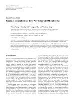
the superimposed training sequence. Figure 1 shows the sim-
ulation results. It is seen that as α decreases (i.e., training
power increases relative to the information sequence power),
one gets better results. Moreover, the proposed method
works with overfitting. Finally, adding nonzero mean (dc off-
set) to additive noise y ielded essentially identical results (dif-
ferences do not show on the plotted curves).
Example 2. Consider (1)withN

=1andL = 2. We simu-
late a random time-and frequency-selective Rayleigh fading
channel following [20]. For different l’s, h(n; l)’s are mutually
independent and for a given l, we follow the modified Jakes’
model [20] to generate h(n; l):
h(n; l)
= X(t)|
t=nT
s
, (57)
where X(t)
= (2/
√
M)

M
i
=1
e
jψ
i
cos(2πf
d
t cos(α
i
)+φ), α
i
=
(2πi−π+θ)/(4M), i = 1, 2, , M, random variables θ, φ,and
ψ

i
are mutually independent (∀i) and uniformly distributed
Jitendra K. Tugnait et al. 7
0 2 4 6 8 10 12 14
20
15
10
5
0
SNR (dB)
Channel MSE (dB)
Power loss = 2dB
Power loss
= 1dB
Power loss
= 0.5dB
Power loss
= 0.2dB
Figure 1: Example 1. Normalized channel MSE (53)basedonT =
140 symbols per run, 100 Monte Carlo runs, QPSK signal, P = 7.
Power loss
=−10 log(α)dBwhereα is as in (55).
over [0, 2π), T
s
denotes the symbol interval, f
d
denotes the
(max.) Doppler spread, and M
=25. For a fixed l,(57)gen-
erates a random process

{h(n; l)}
n
whose power spectrum
approximates the Jakes’ spectrum as M
↑∞. We consider
a system with carrier frequency of 2 GHz, data rate of 40 kB
(kB
= kilo-Bauds), therefore, T
s
= 25 × 10
−6
seconds, and a
varying Doppler spread f
d
in the range 0 Hz to 200 Hz (cor-
responding to a maximum mobile velocity in the range 0 to
108 km/hr). We picked a data record length of 400 symbols
(time duration of 10 msec). For a given Doppler spread, we
pick Q as in Section 1.1 (T
= 400, L = 2in(7)). For the cho-
sen parameters it varies within the values
{1, 3, 5}.Weem-
phasize that the CE-BEM was used only for processing at the
receiver; the data were generated using (57).
We take all sequences (information and training) to
be binary. For superimposed training, we take a p eriodic
(scaled) binary sequence of period P
= 7 with the training-
to-information sequence power ratio (TIR) of 0.3where
TIR

=
σ
2
c
σ
2
b
= α
−1
− 1 (58)
and σ
2
b
and σ
2
c
denote the average power in the information
sequence
{b(n)} and training sequence {c(n)},respectively.
Complex white zero-mean Gaussian noise was added to the
received signal and scaled to achieve a target bit SNR at the
receiver (relative to the contribution of
{s(n)}).
For comparison, we consider conventional time-multi-
plexed training assuming time-invariant channels, as well as
CE-BEM-based periodically placed time-multiplexed train-
ing with and without zero-padding, following [7]. In the for-
mer, the block of data of length 400 symbols was split into
two nonoverlapping blocks of 200 symbols each. Each sub-
block had a training sequence length of 46 symbols in the

middle of the data subblock with 154 symbols for informa-
tion; this leads to a training-to-information sequence power
ratio (over the block length) of approximately 0.3. Assuming
synchronization, time-invariant channels were estimated us-
ing conventional training and used for information detection
via a Viterbi algorithm; this was done for each subblock. In
the CE-BEM set-up, following [7], we took a training block
of length 2L +1
= 5 and a data block of length 17 bits lead-
ing to a frame of length 22 bits. This fr a me was repeated over
the entire record length (22
× 18). Thus, we have a training-
to-information bit ratio of approximately 0.3. Two versions
of training sequences were considered. In one of them zero-
padding was used with a random bit in the middle of the
training block, as in [7]: this leads to a peak-to-average power
ratio (PAR) of 5. In the other version we had a random binary
sequence of length 5 in each training block, leading to a PAR
of 1 (an ideal choice). Assuming synchronization, CE-BEM
channel was estimated using conventional training and used
for information detection via a Viterbi algorithm. We also
considered another variation of zero-padded training with a
training block of length 2L +1
= 5 but a data block of length
50 bits leading to a training-to-information bit ratio of 0.1.
Thus the proposed superimposed training scheme results in a
data transmission rate that is 30% higher than the data trans-
mission rate in all of the time-multiplexed training schemes
considered in this example, except for the last scheme com-
pared to which the data transmission rate is 10% higher.

Figure 2 shows the BER (bit error rate) based on 500
Monte Carlo runs for conventional training based on time-
invariant (TI) modeling, the CE-BEM-based periodically
placed time-multiplexed training for PAR = 5andPAR=
1, the first-order statistics and superimposed training-based
method and the proposed DML approach with two itera-
tions, under varying Doppler spreads f
d
and a bit SNR of
25 dB. It is seen that as Doppler spread f
d
increases beyond
about 60 Hz (normalized Doppler T
s
f
d
of 0.0015), superim-
posed training approach of Section 2 (step (1)) outperforms
the conventional (midamble) training with time-invariant
channel approximation, without decreasing the data trans-
mission rate. Furthermore, the proposed DML enhancement
can lead to a significant improvement with just one iteration.
On the other hand, the CE-BEM-based periodically placed
time-multiplexed training approach of [7] significantly out-
performs the superimposed t raining-based approaches, but
at the cost of a reduction in the data transmission rate.
Figure 3 shows the normalized channel mean-square error
(NCMSE), defined (before averaging over runs) as
NCMSE
=


T
n=1

2
l=0



h(n; l) −h(n; l)


2

T
n
=1

2
l
=0


h(n; l)


2
. (59)
It is seen that the proposed DML enhancement leads to a
significant improvement in channel estimation also with just

one iteration.
8 EURASIP Journal on Applied Signal Processing
0 20 40 60 80 100 120 140 160 180 200
10
6
10
5
10
4
10
3
10
2
10
1
10
0
f
d
(Doppler spread, Hz)
BER
Conv. training, TI model: 46 + 46 bits in the middle
Superimposed training: step 1, TIR
= 0.3
Superimposed training: 1st iteration, TIR
= 0.3
Superimposed training: 2nd iteration, TIR
= 0.3
Conv. training, TV model, PAR
= 5, TIR = 0.1

Conv. training, TV model, PAR
= 5, TIR = 0.3
Conv. training, TV model, PAR
= 1, TIR = 0.3
SISO system; data 400
500; SNR = 25 dB; Viterbi algorithm
Figure 2: Example 2. BER: circle: estimate channel using superimposed training (training-to-information symbol power ratio TIR = 0.3)
and then design a Viterbi detector; square: first iteration specified by step (2) (Section 3); up-triangle: second iteration specified by step
(2) (Section 3); dot-dashed: estimate channel using conventional time-multiplexed training of length 46 bits in the middle of a subblock of
length 200 bits and then design a Viterbi detector; cross: CE-BEM-based periodically placed time-multiplexed training with zero padding
[7], TIR
= 0.3; star: CE-BEM-based periodically placed time-multiplexed training without zero padding, TIR = 0.3; down-triangle: CE-
BEM-based periodically placed time-multiplexed training with zero-padding [7], TIR
= 0.1. SNR = 25 dB. Record length = 400 bits. Results
are based on 500 Monte Carlo runs.
0 20 40 60 80 100 120 140 160 180 200
50
45
40
35
30
25
20
15
10
5
0
f
d
(Doppler spread, Hz)

NCMSE (dB)
Superimposed training: step 1, TIR = 0.3
Superimposed training: 1st iteration, TIR
= 0.3
Superimposed training: 2nd iteration, TIR
= 0.3
Conv. training, TV model, PAR
= 5, TIR = 0.1
Conv. training, TV model, PAR
= 5, TIR = 0.3
Conv. training, TV model, PAR
= 1, TIR = 0.3
SISO system; data 400
500; SNR = 25 dB; Viterbi algorithm
Figure 3: Example 2.AsinFigure 2 except that NCMSE (normalized channel mean-square error) (59) is shown.
Jitendra K. Tugnait et al. 9
0 5 10 15 20 25 30
10
3
10
2
10
1
10
0
SNR (dB)
BER
Superimposed training: 2nd iteration, TIR = 0.3
Conv. training, TV model, PAR
= 5, TIR = 0.1

Conv. training, TV model, PAR
= 5, TIR = 0.3
SISO system; data 400
500; f
d
= 120 Hz; Viterbi algorithm
Figure 4: Example 3. BER for varying SNR with Doppler spread f
d
= 120 Hz: up-triangle: superimposed training, second iteration specified
by step (2) (Section 3), TIR
= 0.3; cross: CE-BEM-based periodically placed time-multiplexed training with zero padding [7], TIR = 0.3;
down-triangle: CE-BEM-based periodically placed time-multiplexed training w ith zero padding [7], TIR
= 0.1. After estimating the channel,
we design a Viterbi detector using the estimated channel. Record length
= 400 bits. Results are based on 500 Monte Carlo runs.
0 5 10 15 20 25 30
16
14
12
10
8
6
4
2
0
2
4
SNR (dB)
NCMSE (dB)
Superimposed training: 2nd iteration, TIR = 0.3

Conv. training, TV model, PAR
= 5, TIR = 0.1
Conv. training, TV model, PAR
= 5, TIR = 0.3
SISO system; data 400
500; f
d
= 120 Hz; Viterbi algorithm
Figure 5: Example 3.AsinFigure 4 except that corresponding NCMSE (normalized channel mean-suare error) (59)isshown.
Example 3. To further compare the relative advantages and
disadvantages of CE-BEM-based superimposed training and
periodically placed time-multiplexed training, we now repeat
Example 2 but with varying SNR; the other details remain
unchanged. Figures 4 and 5 show the simulation results for
a Doppler spread of 120 Hz (normalized Doppler spread of
0.003 for bit duration of T
s
= 25 μs) where we compare
the results of the second iteration of the proposed DML ap-
proach based on superimposed training with that of peri-
odically placed time-multiplexed training. There is an error
floor with increasing SNR which is attributable to modeling
errors in approximating the Jakes’ model with CE-BEM. It is
seen from Figure 4 that our proposed approach outperforms
(better BER) the CE-BEM-based periodically placed time-
multiplexed training approach of [7] for SNRs at or below
10 dB, and underperforms for SNRs at or above 20 dB. There
is also the data transmission rate advantage at al l SNRs.
5. CONCLUSIONS
In this paper we first presented and extended the first-order

statistics-based approach of [17] for time-varying (CE-BEM
10 EURASIP Journal on Applied Signal Processing
based) channel estimation using superimposed training.
Then we extended the first-order statistics-based solution
to an iterative approach to joint channel and information
sequence estimation, based on CE-BEM, using Viterbi de-
tectors. The first-order statistics-based approach views the
information sequence as interference whereas in the itera-
tive joint estimation version it is exploited to enhance chan-
nel estimation and information sequence detection. The re-
sults were illustrated via several simulation examples some of
them involving time-and frequency-selective Rayleigh fading
where we compared the proposed approaches to some of the
existing approaches. Compared to the CE-BEM-based per i-
odically placed time-multiplexed training approach of [7],
oneachievesalowerBERforSNRsatorbelow10dB,and
higher BER for SNRs at or above 20 dB. There is also the
data transmission rate advantage at all SNRs. Further work
is needed to compare the relative advantages and disadvan-
tages of CE-BEM-based superimposed training and periodi-
cally placed time-multiplexed training.
ACKNOWLEDGMENTS
This work was supported by the US Army Research Office
under Grant DAAD19-01-1-0539 and by NSF under Grant
ECS-0424145. Preliminary versions of the paper were pre-
sented in parts at the 2003 and the 2004 IEEE International
Conferences on Acoustics, Speech, Signal Processing, Hong
Kong, April 2003 and Montreal, May 2004, respectively.
REFERENCES
[1] M A. R. Baissas and A. M. Sayeed, “Pilot-based estimation

of time-varying multipath channels for coherent C DMA re-
ceivers,” IEEE Transactions on Signal Processing, vol. 50, no. 8,
pp. 2037–2049, 2002.
[2] I. Barhumi, G. Leus, and M. Moonen, “Time-varying FIR
equalization for doubly selective channels,” IEEE Transactions
on Wireless Communications, vol. 4, no. 1, pp. 202–214, 2005.
[3] B. Farhang-Boroujeny, “Pilot-based channel identification:
proposal for semi-blind identification of communication
channels,” Electronics Letters, vol. 31, no. 13, pp. 1044–1046,
1995.
[4] G. B. Giannakis and C. Tepedelenlioglu, “Basis expansion
models and diversity techniques for blind identification and
equalization of time-varying channels,” Proceedings of the
IEEE, vol. 86, no. 10, pp. 1969–1986, 1998.
[5] G. Leus, “Semi-blind channel estimation for rapidly time-
varying channels,” in Proceedings of the IEEE International
Conference on Acoustics, Speech, and Signal Processing (ICASSP
’05), vol. 3, pp. 773–776, Philadelphia, Pa, USA, March 2005.
[6] X. Ma and G. B. Giannakis, “Maximum-diversity transmis-
sions over doubly selective wireless channels,” IEEE Transac-
tions on Information Theor y, vol. 49, no. 7, pp. 1832–1840,
2003.
[7] X. Ma, G. B. Giannakis, and S. Ohno, “Optimal training
for block transmissions over doubly selective wireless fad-
ing channels,” IEEE Transactions on Signal Processing, vol. 51,
no. 5, pp. 1351–1366, 2003.
[8] X. Meng and J. K. Tugnait, “Superimposed training-based
doubly-selective channel estimation using exponential and
polynomial bases models,” in Proceedings of the 38th Annual
Conference on Information Sciences & Systems (CISS ’04),

Princeton University, Princeton, NJ, USA, March 2004.
[9] A.G.Orozco-Lugo,M.M.Lara,andD.C.McLernon,“Chan-
nel estimation using implicit training,” IEEE Transactions on
Signal Processing, vol. 52, no. 1, pp. 240–254, 2004.
[10] B. Porat, Digital Processing of Random Signals, Prentice-Hall,
Englewood Cliffs, NJ, USA, 1994.
[11] J. G. Proakis, Digital Communications, McGraw-Hill, New
York, NY, USA, 4th edition, 2001.
[12] P. Schniter, “Low-complexity equalization of OFDM in dou-
bly selective channels,” IEEE Transactions on Signal Processing,
vol. 52, no. 4, pp. 1002–1011, 2004.
[13] N. Seshadri, “Joint data and channel estimation using blind
trellis search techniques,” IEEE Transactions on Communica-
tions, vol. 42, no. 2–4, part 2, pp. 1000–1011, 1994.
[14] P. Stoica and R. L. Moses, Introduction to Spectral Analysis,
Prentice-Hall, Englewood Cliffs, NJ, USA, 1997.
[15] M. K. Tsatsanis and G. B. Giannakis, “Modeling and equaliza-
tion of rapidly fading channels,” International Journal of Adap-
tive Control & Signal Processing, vol. 10, no. 2-3, pp. 159–176,
1996.
[16] J. K. Tugnait and W. Luo, “On channel estimation using super-
imposed training and first-order statistics,” IEEE Communica-
tions Letters, vol. 7, no. 9, pp. 413–415, 2003.
[17]
, “On channel estimation using superimposed train-
ing and first-order statistics,” in Proceedings of the IEEE Inter-
national Conference on Acoustics, Speech and Signal Processing
(ICASSP ’03), vol. 4, pp. 624–627, Hong Kong, April 2003.
[18] J. K. Tugnait and X. Meng, “On superimposed training for
channel estimation: performance analysis, training power al-

location, and frame synchronization,” IEEE Transactions on
Signal Processing, vol. 54, no. 2, pp. 752–765, 2006.
[19] J. K. Tugnait, L. Tong, and Z. Ding, “Single-user channel es-
timation and equalization,” IEEE Signal Processing Magazine,
vol. 17, no. 3, pp. 16–28, 2000.
[20] Y. R. Zheng and C. Xiao, “Simulation models with correct sta-
tistical properties for Rayleigh fading channels,” IEEE Transac-
tions on Communications, vol. 51, no. 6, pp. 920–928, 2003.
[21] G. T. Zhou, M. Viberg, and T. McKelvey, “A first-order statis-
tical method for channel estimation,” IEEE Signal Processing
Letters, vol. 10, no. 3, pp. 57–60, 2003.
Jitendra K. Tugnait received the B.S. degree
with honors in electronics and electrical
communication engineering from the Pun-
jab Engineering College, Chandigarh, India,
in 1971, the M.S. and the E.E. degrees from
Syracuse University, Syracuse, NY, and the
Ph.D. deg ree from the University of Illinois
at Urbana-Champaign, in 1973, 1974, and
1978, respectively, all in electrical engineer-
ing. From 1978 to 1982, he was an Assistant
Professor of electrical and computer engineering at the University
of Iowa, Iowa City, Iowa. He was with the Long Range Research Di-
vision of the Exxon Production Research Company, Houston, Tex,
from June 1982 to September 1989. He joined the Department of
Electrical and Computer Engineering, Auburn University, Auburn,
Aa, i n September 1989 as a Professor. He currently holds the title
of James B. Davis Professor. His current research interests are in
statistical signal processing, wireless and wireline digital commu-
nications, multiple-sensor multiple-target tracking, and stochastic

systems analysis. Dr. Tugnait is a past Associate Editor of the IEEE
Transactions on Automatic Control and of the IEEE Tr ansactions
Jitendra K. Tugnait et al. 11
on Signal Processing. He is currently an Editor of the IEEE Transac-
tions on Wireless Communications and an Associate Editor of IEEE
Signal Processing Letters. He was elected Fellow of IEEE in 1994.
Xiaohong Meng was born in Luoyang,
He’nan Province, China, on June 12, 1973.
She received her B.E. degree in 1995 in elec-
trical engineering from Beijing University of
Posts and Telecommunications. From 1995
to 1999, she held the position of Instruc-
tor at He’nan Posts and Telecommunica-
tions School. From September 1995 to June
2001, she studied as a graduate student at
Beijing University of Posts and Telecommu-
nications. From January 2002 to May 2005, she was a Research
Assistant in Electrical and Computer Engineering Department of
Auburn University. She received her Ph.D. degree in electrical en-
gineering in May 2005 and her M.S. degree in mathematics in
May 2006 from Auburn University. She joined MIPS Technologies,
Mountain View, Calif, in March 2006. Her current research inter-
ests include digital signal processing, statistical signal processing,
wireless communications, and semiblind equalization.
Shuangchi He received the B.E. and M.S.
degrees in electronic eng ineering from Ts-
inghua University, Beijing, China, in 2000
and 2003, respectively. He is currently
working towards his Ph.D. degree in electri-
cal engineering at Auburn University. Since

2003, he has been a Graduate Research As-
sistant at the Department of Electrical and
Computer Engineering, Auburn University.
His research interests include channel esti-
mation and equalization, multiuser detection, and statistical and
adaptive signal processing and analysis.