Báo cáo hóa học: " Advanced Integration of WiFi and Inertial Navigation Systems for Indoor Mobile Positioning" doc
Bạn đang xem bản rút gọn của tài liệu. Xem và tải ngay bản đầy đủ của tài liệu tại đây (1.66 MB, 11 trang )
Hindawi Publishing Corporation
EURASIP Journal on Applied Signal Processing
Volume 2006, Article ID 86706, Pages 1–11
DOI 10.1155/ASP/2006/86706
Advanced Integration of WiFi and Inertial Navigation Systems
for Indoor Mobile Positioning
Fr
´
ed
´
eric Evennou and Franc¸ois Marx
Division R&D, TECH/IDEA, France Telecom, 38243 Meylan, France
Received 23 June 2005; Revised 23 January 2006; Accepted 29 January 2006
This paper presents an aided dead-reckoning navigation structure and signal processing algorithms for self localization of an
autonomous mobile device by fusing pedestrian dead reckoning and WiFi signal s trength measurements. WiFi and inertial navi-
gation systems (INS) are used for positioning and attitude determination in a wide range of applications. Over t he last few years,
a number of low-cost inertial sensors have become available. Although they exhibit large errors, WiFi measurements can be used
to correct the drift weakening the navigation based on this technology. On the other hand, INS sensors can interact with the WiFi
positioning system as they provide high-accuracy real-time navigation. A structure based on a Kalman filter and a particle filter
is proposed. It fuses the heterogeneous information coming from those two independent technologies. Finally, the benefits of the
proposed architecture are evaluated and compared with the pure WiFi and INS positioning systems.
Copyright © 2006 Hindawi Publishing Corporation. All rights reserved.
1. INTRODUCTION
Mobile positioning becomes of increasing interest for the
wireless telecom operators. Indeed, many applications re-
quire an accurate location information of the mobile
(context-aware application, emergency situation, etc.). While
many outdoor solutions exist, based on GPS/AGPS, in in-
door environments, the received signals are too weak to pro-
vide an accurate location using those technologies. Currently,
given that many buildings are equipped with WLAN access
points (shopping malls, museums, hospitals, airports, etc.),
it may become practical to use these access points to deter-
mine user location in these indoor environments. Moreover,
new regulations will impose to VoWiFi (voice over WiFi) op-
erators to integrate a positioning solution in their terminals
to comply with the E911 policy [1]. The location technique
is based on the measurement of the received signal strength
(RSS) and the well-known fingerprinting method [2, 3]. The
accuracy depends on the number of positions registered in
the database. Besides, signal fluctuations over time introduce
errors and discontinuities in the user’s trajectory.
To minimize the fluctuations of the RSS, some filtering is
needed. A simple temporal averaging filter does not give sat-
isfying results. Kalman filtering [4, 5] is commonly used in
automatic control to track the trajectory of a target. How-
ever, more information can be used to improve the accu-
racy. In the following sections, we choose to use a map of the
environment. It is used in order to find the most probable
trajectory of the mobile and avoid wall crossings. Including
such information requires new filters as the Kalman filter is
not adapted for this. Particle filters [6–8], based on Monte-
Carlo simulations, are emerging to solve the problems of po-
sition estimation.
Inertial navigation systems (INS) are one of the most
widely used dead-reckoning systems. They can provide con-
tinuous position, velocity, and also orientation estimates,
which are accurate for a short term, but are subject to drift
due to noise of the sensor [9, 10]. Filtering techniques will
limit the effect of the measurement noise and therefore re-
duce this drift. The Kalman filter is already used in many
GPS/INS applications, to reduce the effect of this measure-
ment noise. Merging positioning information from two so
different technologies must lead to very interesting results.
Moreover, the strength of the INS system should annihilate
the weaknesses of WiFi and vice versa. Those heterogenous
but complementary technologies should lead to an enhanced
system in terms of positioning performance as well as avail-
ability of the positioning service over a larger area. Indeed,
when the WiFi positioning is unavailable because of network
uncovered area, the dead-reckoning system can go on and
provide a position estimate which is degraded over the time
but can be reliable over a certain period.
This paper presents in its second section the basic tech-
niques leading to a first estimate of the position of a WiFi
device thanks to the associated network. The third section
introduces a convenient way based on the use of the particle
2 EURASIP Journal on Applied Signal Processing
filtertoreducetheeffect of the WiFi measurement noise and
to integr a te more information such as the map of a building.
Section 4 presents our system based on dead-reckoning nav-
igation, and will use information from a dual axis accelerom-
eter, a gyroscope, and a pressure sensor. The next section
demonstrates the capability of the particle filter to integrate
information of those two different technologies and combine
them efficiently to lead to a more performing system. Finally,
Section 6 gives some information about the performance of
all those different systems, when used separately, and coop-
eratively.
2. BASIC INDOOR MOBILE POSITIONING WITH WIFI
Many outdoor systems are based on time measurements, that
is, the mobile equipment and the network are synchronized.
Thus, the mobile can calculate its distance from the access
point (AP).
However getting this kind of information with off-the-
shelf WiFi equipments is almost impossible. The only avail-
able information is the signal strength received from each AP.
Indeed, the received signal strength is measured and is one of
the outputs of the card. Such information is available because
the APs send beacons periodically. Mobile devices use those
beacons to handle the roaming inside the network. Given this
consideration, it is possible to get a list of the received power
coming from all the APs covering the area where the mobile
is moving.
2.1. Signal strength and propagation model
The reception of a tuple of signal strengths does not lead di-
rectly to the position of the device. A conversion of this tuple
of received signal strengths into a position is required. The
Motley-Keenan propagation model is a convenient propaga-
tion model often used for its simplicity. This model is pre-
sented in [11]; its simplest form is given by
P
received
d
= P
received
d
0
− 10 · α · log
d
d
0
,(1)
where P
received
d
is the signal strength received by the mobile
at distance d, P
received
d
0
the signal strength received at the
known distance d
0
from the AP, and α acoefficient modeling
the radio wave propagation in the environment. For exam-
ple, in free path loss environment, we have α
= 2. In indoor
environments, this factor will be closer to 3 [12].
This model is rather simple and needs only two param-
eters, that is, P
received
d
0
and α. Ranging experiments were
carried out using this propagation model, but a very poor
accuracy was obtained, probably due to the too simple form
of this m odel, in comparison to the complex radio environ-
ment.
Refinements of this model exist. They introduce some
wall attenuation factors, but some extra information is
needed [3] to describe more closely the environment. The
walls’ materials must be characterized, and their properties
must be introduced in the model, leading to the following
approximation [3]:
P
received
(d) = P
received
d
0
−
10 · α · log
d
d
0
+
N
w
i=0
n
i
· ω
i
,
(2)
where N
w
− 1 is the number of walls of different nature, n
i
is the number of walls having an attenuation of ω
i
dB. Such
a propagation model leads to a better estimate of the range
separating the mobile from each AP, but requires more ef-
forts to calibrate. Combining those estimated ranges with a
multilateration algorithm, it is possible to find the position
of the mobile.
Further investigations showed that introducing the es-
timated ranges, obtained with the propagation models de-
scribed above, in a multilateration algorithm leads to a poor
positioning due to the large estimation errors. Those errors
appear because the propagation models are too simple in
comparison to the complex indoor RF propagation.
2.2. WiFi cell ID, signal strength and fingerprinting
The simplest approach for locating a m obile device in a
WLAN environment is to approximate its position by the po-
sition of the access point received at that position with the
strongest signal strength. The major benefit of such a system
is its simplicity, but its main drawback is its large estimation
error. The accuracy is proportional to the density of access
points, which is in the range of 25 to 50 meters for indoor
environments [13]. Reference [2] introduced a different ap-
proach for locating the dev i ce in indoor environments by us-
ing the radio signal strength fingerprinting.
Fingerprinting positioning is a quite different technique.
It consists in having some signal power footprints or sig na-
tures that define a position in the environment. This signa-
ture is made of the received signal powers from different ac-
cess points that cover the environment. A first step, called
training or profiling, is necessary to build this mapping be-
tween collected received signal strength and certain positions
in the building. This leads to a database that is used during
the positioning phase. Building the footprint database can
be done in two ways. A first method is to do on-site mea-
surements for some reference positions in the building with
a user terminal. An alternative approach is based on collect-
ing limited on-site measurements and introducing them in a
tunable propagation model that would use them to fit some
of its parameters. Then, this propagation model gives an ex-
tensive coverage map for each AP. However, the poor results
obtained earlier with the use of the propagation model did
not invite us to focus on such a model. Neural networks are
another learning method for improving propagation mod-
elsovertime[14]. It was decided to carry on with the use
of the data collected to build the database. Ray tracing tools
represent another solution to build such a database, but they
are very complex tools. Moreover, a good knowledge of the
radio environment (knowledge of the presence and position
of all the APs) is needed to cope with the interfering issue.
F. Evennou and F. Marx 3
However, such information is not always available due to the
fast growing emergence of this technology in indoor environ-
ments.
Once this prerequisite step is accomplished, it is neces-
sary to do the reversing operation, which will deliver the po-
sition associated to an instantaneous collected tuple of re-
ceived signal strengths. Different techniques can fit these re-
quirements.
2.2.1. k-closest neighbors fingerprinting
This algorithm goes through the database and picks the k
referenced positions that match best the observed received
signal strength tuple. The criterion that is commonly re-
tained is the Euclidian distance (in signal space) metric. If
Z
=
RSS
1
, ,RSS
M
is the observed RSS vector com-
posed of M received access points at the unknown position
X
= (x, y)andZ
i
the footprint recorded in the database for
the position X
i
=
x
i
, y
i
, then this Euclidian distance is
d
Z, Z
i
=
1
M
·
M
j=1
RSS
j
(x, y) −RSS
j
x
i
, y
i
2
,(3)
where RSS
j
x
i
, y
i
is the mean value recorded in the database
for the access point whose MAC address is noted “ j” at the
position
x
i
, y
i
.
The set N
k
of the database positions having the smallest er-
rors is built with an iterative process as follows:
N
k
=
argmin
X
i
∈L
d
Z, Z
i
\ X
i
/∈ N
k−1
,(4)
where L is the set of positions recorded in the database. This
set contains k positions. Finally, the position of the mobile is
considered to be the barycenter of those k selected positions:
X
=
k
j=1
1/d
Z, Z
i
·
X
j
k
j=1
1/d
Z, Z
i
with X
j
∈ N
k
. (5)
The main advantage of this method is its simplicity to set
it up. However the accuracy highly depends on the granu-
larity of the reference database [15]. A better accuracy can
be achieved with finer grids, but a finer grid means a larger
database that is more time costly.
2.2.2. Probabilistic estimation
The main drawback of the nearest neighbor method is its lack
of accuracy when the size of the database is limited. A prob-
abilistic approach has been proposed in [16, 17]. This ap-
proach is based on an empirical model that describes the dis-
tribution of received signal strength at various locations. The
use of probabilistic models provides a natural way to handle
uncertainty and errors in signal power measurements. Thus,
after the calibration phase, for any given location X,aprob-
ability distribution Pr
Z | X
assigns a probability for each
measured signal vector Z. Applying the Bayes rule leads to
the following posterior distribution of the location [ 16 ]:
Pr
X | Z
=
Pr
Z | X
·
Pr
X
Pr
Z
=
Pr
Z | X
·
Pr
X
X
i
∈L
Pr
Z | X
i
·
Pr
X
i
,
(6)
where Pr
X
is the prior probability of being at location l be-
fore knowing the value of the observation variable, and the
summation goes over the set of possible location values, de-
noted by L.
The prior distribution Pr
X
gives a simple way to incor-
porate background information, such as personal user pro-
files, and to implement tracking. In case neither user profiles
nor a history of measured signal properties allowing track-
ing are available, one can simply use a uniform prior which
introduces no bias towards any particular location. As the de-
nominator Pr
Z
does not depend on the location variable
l, it can be treated as a normalizing constant whenever only
relative probabilities or probability ratios are required.
The posterior distribution Pr
X | Z
can be used to
choose an optimal estimator of the location based on what-
ever loss function is considered to express the desired be-
havior. For instance, the squared error penalizes large errors
more than small ones, which is often useful. If the squared
error is used, the estimator minimizing the expected loss is
the expected value of the location variable:
E
X | Z
=
X
i
∈L
l · Pr
X | Z
(7)
assuming that the expectation of the location variable is well
defined, that is, the location variable is numer ical. Location
estimates, such as the expectation, are much more useful
if they are complemented with some indication about their
precision.
However, in both techniques, the signal strength fluctu-
ations (Figure 1) introduce many unexpected jumps in the
final trajector y. Removing those jumps can be done by us-
ing a filter. Kalman filter and particle filter are often used in
parameter estimating problems and tracking. This last filter
will be introduced in the next section, and the benefits using
such a filter will be presented.
3. IMPROVING WIFI POSITIONING WITH
A PARTICLE FILTER
Nowadays, the maps of all the public or company buildings
are available in digital format (dxf, jpeg, etc.). The key idea is
to combine the motion model of a person and the map infor-
mation in a filter in order to obtain a more realistic trajectory
and a smaller error for a trip around the building. In the fol-
lowing, it will be considered that the map, which is available,
is a bitmap. So no information is available except the pixels
in black and white which model the structure of the build-
ing. The particle filter, based on a set of random weighted
samples (i.e., the particles), represents the density function
of the mobile position. Each particle explores the environ-
ment according to the motion model and map information.
4 EURASIP Journal on Applied Signal Processing
−50−55−60−65−70−75−80−85−90−95
Received power (dBm)
0
0.05
0.1
0.15
0.2
0.25
Probability distribution of RSS
Histogram of t he RSS for 00:06:25:49:A9:07
(a)
−60−65−70−75−80−85−90−95−100−105
Received power (dBm)
0
0.05
0.1
0.15
0.2
0.25
0.3
0.35
Probability distribution of RSS
Histogram of t he RSS for 00:06:25:4A:A2:EF
(b)
Figure 1: Received signal strength variations over time for two dif-
ferent access points and for the same position.
Their weights are updated each time a new measurement is
received. It is possible to forbid some moves like crossing the
walls by forcing the weight at 0 for the particles having such
abehavior.
The particle filter tries to estimate the probability distri-
bution Pr
x
k
| Z
0:k
,wherex
k
is the state vector of the device
at the time step k,andZ
0:k
is the set of collected measure-
ments until the (k + 1)th measurement. When the number of
particles (position x
i
k
,weightw
i
k
) is high, the discrete proba-
bility density function of presence can be assimilated to
Pr
x
k
| Z
0:k
=
N
s
i=1
w
i
k
δ
x
k
− x
i
k
. (8)
This filter comprises two steps:
(i) prediction;
(ii) correction.
3.1. Prediction
During this step, the particles propagate across the building
given an evolution law that assigns a new position for each
particle with an acceleration governed by a random process:
⎡
⎢
⎢
⎢
⎣
x
k+1
y
k+1
v
x
k+1
v
y
k+1
⎤
⎥
⎥
⎥
⎦
=
⎡
⎢
⎢
⎢
⎣
10T
s
0
01 0 T
s
00 1 0
00 0 1
⎤
⎥
⎥
⎥
⎦
⎡
⎢
⎢
⎢
⎣
x
k
y
k
v
x
k
v
y
k
⎤
⎥
⎥
⎥
⎦
+
⎡
⎢
⎢
⎢
⎢
⎢
⎢
⎣
T
2
s
2
000
0
T
2
s
2
00
00T
s
0
000T
s
⎤
⎥
⎥
⎥
⎥
⎥
⎥
⎦
⎡
⎢
⎢
⎢
⎣
η
x
k
η
y
k
η
x
k
η
y
k
⎤
⎥
⎥
⎥
⎦
,
(9)
where
x
k
, y
k
, v
x
k
, v
y
k
T
denotes the state vector associated
to each particle (position and speed), T
s
the elapsed time
between the (k
− 1)th and the kth WiFi measurements.
η
x
k
, η
y
k
, η
x
k
, η
y
k
T
is a random process that simulates the ac-
celeration of the kth particle. This last equation is often called
the prior equation. It has the form of the movement law
(Newton’s laws) given by x
k
= x
k−1
+ v · T
s
+ a ·T
2
s
/2, where
a is the acceleration of the mobile and v its velocity. Here
the particles are given a ra ndom exploration move thanks to
the acceleration random process. It tries to predict a new po-
sition for all the particles. The used process is a zero mean
Gaussian noise whose variance must be realistic of a pedes-
trian movement.
When the new position of a par ticle is known, it is pos-
sible to include the map information, in order to remove the
particles having an impossible move, like crossing a wall. An
algorithm, using the previous known position of the particle,
its new one, plus the map of the building, checks all the pix-
els between those positions to see if a wall has been crossed.
This processing is time consuming as it must be done for each
particle at each time step. When this checking is finished, it
is possible to assign a weight Pr[x
k
| x
k−1
] as follows:
Pr
x
k
| x
k−1
=
⎧
⎨
⎩
P
m
if a particle crossed a wall,
1
− P
m
if a particle did not cross a wall.
(10)
Since crossing a wall is impossible for a normal user, it has
been decided to take P
m
= 0. Then, the particles disappear
when the y cross a wall. A common problem with the par-
ticle filter is the degeneracy phenomenon: after a few iter-
ations, many particles will have a negligible weight. A re-
sampling step will occur when the degeneracy is too severe
(see Section 3.4).
3.2. Correction
When a measurement (tuple of RSS) is available, it must be
taken into account to correct the weight of the particles in
order to approximate Pr
x
k
| Z
0:k
. As the measurement is
made of signal strengths and given that particles are charac-
terized by their position, the RSS tuple must be transformed
F. Evennou and F. Marx 5
into a position. The mapping between the position and the
signal strengths is performed thanks to the empirical fin-
gerprinting database. In fact, the algorithm used in Section
2.2 to find the position of the mobile, given the RSS cov-
erage in the building , is used. Then it is possible to esti-
mate Pr
Z
k
| x
k
. In the case of an indoor movement, the
closest neighbor algorithm returns a position denoted X
z
k
(see Section 2.2.1), which matches the current WiFi mea-
surement. This last position, equivalent to the measurement,
is introduced in the weight of the particles as follows:
Pr
Z
k
| x
i
k
=
1
√
2πσ
exp
−
X
z
k
− X
x
i
k
2
2 · σ
2
(11)
with X
z
k
being the position returned by the database, X
x
i
k
the
position of the ith particle at time step k,andσ the measure-
ment confidence. The smaller σ will be, the more confident
the user is in the measurement. That would mean that there
are very little variations in the measurements for the same
position. Here, σ is chosen depending on the variations of
the RSS. It can be noticed that with this Gaussian law, the
closer the particle is to the position returned by the database,
the higher its Pr
Z
k
| x
k
willbe.Now,havingdefinedallthe
necessary probabilities to update the weight of a particle, we
just need to combine them to find the new posterior distri-
bution.
3.3. Particle update
The weight update equation is given in [6, 7]
w
i
k
= w
i
k
−1
· Pr
x
k
| x
k−1
·
Pr
z
k
| x
k
. (12)
To obtain the posterior density function, it is necessary to
normalize those weights. After a few iterations, when too
many particles crossed a wall, just a few particles will be kept
alive (particles with a nonzero weight). To avoid having just
one remaining particle, a resampling step is triggered.
3.4. Resampling
The resampling is a c ritical point for the filter. The basic idea
behind the resampling step is to move the particles that have
a too low weight, in the area of the map where the high est
weights are. This leads to a loss of diversity because many
sampleswillberepeated.Thecriteriontotriggeraresam-
pling is given by
1
N
s
i=0
w
i
k
2
≤ Threshold. (13)
Various resampling algor ithms were proposed. We did not
choose the simple SIS (sequential importance sampling) par-
ticle filter [6], but the resampling approach presented in [18]:
the regularized par ticle filter (RPF). The RPF adds a regu-
larization step. This approach is more convenient because it
locally introduces a new diversity after the resampling. This
may be useful in extreme situations when all the particles are
trapped in a room; whereas the device is still moving along
a corridor. This method of resampling adds a small noise to
the particle position and avoids this phenomenon.
The main stages of the particle filter used in indoor en-
vironments have been presented. To run it, a large number
of particles must be used. This makes the filter very heavy to
processateachtimestepaseveryparticlemustbechecked
for a wall crossing. Due to the large number of particles, the
algorithm is too complex to be implemented on handheld
devices. A way to cut down this number of particles must be
found. Using a new representation of the building is one of
the solutions. The Voronoi diagram of the building has been
used in [19, 20] to reduce the computation complexity of the
particle filter.
4. POSITIONING WITH INERTIAL
NAVIGATION SENSORS
INSs are self-contained, nonradiating, nonjammable, dead-
reckoning navigation systems which provide dynamic infor-
mation through direct measurements. Fundamentally, gyro-
scopes provide angular rate, and accelerometers provide ve-
locity rate information. Although the information rates are
reliable over long periods of time, they must be integr ated
to provide orientation, linear position, and velocity informa-
tion. Thus, even very small errors in the information rates
can cause an unbounded growth in the error of integrated
measurements. One way of overcoming this problem is to use
inertial sensors in conjunction with other absolute sensing
mechanisms to periodically reset them.
In this experiment, the available sensors are: a gyroscope
that delivers some information about the angular speed of
the mobile; a biaxial accelerometer to count the number of
steps, and to detect if it is moving or not; and the last sensor
is an atmospheric pressure sensor, used in detecting when
the mobile is going from one floor to the other. Other sen-
sors, like magnetometers, could be added. In order to col-
lect some relevant measurements translating the real moves
of the pedestrian, the sensing box needs to b e attached to a
part of the body that is only affected by the moves of the user.
The belt (or the hips) is an interesting part of the body for
collecting information about the behavior of the user.
Interests in such a positioning technolog y increase be-
cause mobile phones start integrating such systems [21].
Users often have their mobile phone at the belt, so it would
be possible to use those sensors in order to get an estimate of
their position.
Here the accelerometer has been used to count the num-
ber of steps the user did during his trajectory. This is possible
because w hen the user is walking the signal fluctuates peri-
odically as long as he keeps moving at the same speed. Using
a thresholding system, it becomes possible to accurately es-
timate the number of steps the user did. Getting an estimate
of the distance is tougher as it requires a calibration step, and
the hypothesis that all the user’s steps stride are always the
same. However, over a certain distance, such an assumption
seems realistic.
To keep track of the rotation around the z-axis, the an-
gular velocity ω sensed by the gyroscope must be integrated.
6 EURASIP Journal on Applied Signal Processing
Defining θ
z
as the current z-axis relative to the original ori-
entation, we have
θ
z
=
T
0
ω
z
dt. (14)
With this information, it becomes possible to predict the po-
sition of the mobile at each time step, given that the initial
position of the mobile is known when the inertial navigation
sensors are powered. This position is given by
x
k
y
k
=
x
k−1
y
k−1
+ v · ΔT ·
cos
θ
k
sin
θ
k
, (15)
where v is the speed of the mobile resulting from the prod-
uct of the step stride and the step frequency, ΔT the elapsed
time between two angular speed measurements. The step fre-
quency is obtained thanks to the data coming from the ac-
celerometer sensor. Future generation of the system should
be able to estimate this parameter on the fly. θ
k
is the rotation
along the z-axis that occurred during the move of the pedes-
trian. This last parameter is obtained from the gyroscope:
θ
k
=
k
t=0
˙
θ
k
−
˙
θ
k−1
ΔT. (16)
However, a more realistic model must take into account
the measurement noise. This noise represents the weakness
of dead-reckoning positioning system. The quality of this
system is related to the quality of the sensors that are inte-
grated. Indeed, the power of this noise is quite important, as
it generates a deviation on the trajectory. This drift needs to
be corrected in order to avoid such errors.
Here a 2D problem has been considered, but it is possible
to get the third coordinate of the mobile. The atmospheric
pressure sensor incorporated in the sensor box can be used
to measure the pressure variations. Pressure variations are
relevant over a short period. It becomes inconsistent over a
long period as the pressure can change naturally due to the
weather. Thus measuring those variations will lead to know
if the mobile is climbing or going down, and it is possible
to know the elevation of the mobile with the equations de-
scribed in [22–24].
Inertial navigation is a dead-reckoning technique, which
suffers from one serious limitation: drift rate errors con-
stantly accumulating over time. Since its drift errors relent-
lessly accumulate, an inertial navigation system that operates
for an appreciable length of time must be updated period-
ically with fresh positioning information. This can be ac-
complished by using an external navigation reference, such
as WiFi positioning.
5. COOPERATION BETWEEN INS NAVIGATION
AND WIFI POSITIONING SYSTEMS
Combination of GPS and inertial navigation sensors is com-
mon in automotive applications in order to extend the cover-
age of GPS, as dead reckoning keeps delivering the position of
the mobile during GPS unavailability periods. For the WiFi
positioning system presented above, the interest is to get a
better knowledge of the behavior of the mobile in order to re-
duce the effect of the WiFi measurement noise, and to guide
the particles in a smarter way. Combining information com-
ing from those two heterogeneous technologies must lead to
performance improvements for the WiFi positioning system
presented in Section 2, as the behavior of the particles could
be refined with the INS sensors measurements. To optimally
combine the redundant INS information, a Kalman filtering
scheme is used whereby WiFi measurements regularly update
the inertial state vector. A system combining the power of
the WiFi positioning system using a particle filter, with the
filtered INS information coming from a Kalman filter used
to track the INS information, can be suitable to improve the
whole positioning of the mobile.
The form of the particle filter is convenient to introduce
the information coming from the INS sensors. This informa-
tion can guide the particles as they are directly related to the
behavior of the user.
On the other hand, the use of a Kalman filter for the INS
sensors information, particularly for the information com-
ing from the gyroscope, makes it possible to reduce the ef-
fect of the noise affecting this sensor, as the trajectory of
the barycentre of the particles (including the map informa-
tion) can be injected in the Kalman filter to correct this drift.
Figure 2 presents the architecture that has been implemented
to realize an indoor WiFi/INS positioning demonstrator.
Here the smoothing filter is the particle filter and the data
filtering box corresponds to the processing that data coming
from the INS sensors undergo. Integrating the information
coming from the inertial navigation sensor inside the par-
ticle filter seems quite easy as it just requires to change the
prediction (9) as follows:
x
k+1
y
k+1
=
10T
s
· cos
θ
k
01T
s
· sin
θ
k
⎡
⎢
⎣
x
k
y
k
v
k
⎤
⎥
⎦
+
⎡
⎢
⎢
⎣
T
2
s
2
0
0
T
2
s
2
⎤
⎥
⎥
⎦
η
x
η
y
(17)
with v
k
the amplitude of the speed estimated thanks to the
data coming from the accelerometer sensor. θ
k
is the angle
returned by the inertial navigation processing unit. This an-
gle is obtained thanks to the Kalman filter that uses the data
coming from the gyroscope and the angle of the trajectory
delivered by the WiFi positioning system. The following set
of equations presents the Kalman filter that is used in this
application to track the rotation of the mobile:
θ
−
k
= θ
k−1
−
˙
θ
k
· ΔT,
P
−
k
= Q + P
k−1
,
K
k
= P
−
k
·
P
−
k
+ R
−1
,
θ
k
= θ
−
k
+ K
k
θ
trajectory
− θ
−
k
,
P
k
=
1 − K
k
· P
−
k
(18)
with
˙
θ
k
being the angular speed returned by the gyroscope,
θ
k−1
the previous predicted angle, ΔT the time between two
F. Evennou and F. Marx 7
Reference
positioning
database
Set of data coming
from the sensors
WiFi RSS
measurement
Matching
algorithm
Smooth tracking
(particle filter)
Data filtering
(Kalman filter)
Traje c tor y
(position)
Trajectory angle
delivered by the
WiFi system
Figure 2: Block diagram of the INS/WiFi mutually correcting architecture.
measurements from the inertial sensors, as well as Q and R
the covariance matrixes of noises affecting the process and
measurement equations, respectively, describing the Kalman
filter. K
k
represents the Kalman gain. P
−
k
and P
k
denote the
error covariance matrixes, and θ
trajectory
is the angle of the
trajectory returned by the particle filter, related to the WiFi
measurements.
This structure enables sensors to correct one another in
a smart manner. However, if a sensor fails (WiFi due to a de-
graded fingerprinting database), then the whole system will
fail to provide a good estimate of the position of the device as
the system is mainly based on the WiFi positioning. On the
other hand, a failure for the INS system will be less stringent.
Data from INS sensors are just used to indicate the behav-
ior that the particle must follow. This will lead to make the
particles moving in the wrong direction, and then the filter
will trigger a resampling step to concentrate the particles in
the most interesting areas where the mobile is standing. Such
a resampling step will be triggered more often than normal.
Thus, failure of the INS system will lead to a degradation of
the positioning, but will not blind the system. If the WiFi sys-
tem fails to give a correct position then the INS system will
notbeabletocorrectthewholesystem.
The next section presents the results that are obtained by
using all these techniques.
6. PERFORMANCE EVALUATION BASED
ON EXPERIMENTAL RESULTS
Experimentations were conducted to get a better idea of
the p erformances that can be awaited from such positioning
techniques. Experimentations were carried out in a 40*40 m
indoor office building. An access point was standing in each
corner of this building. The mobile terminal was a laptop
on which all these algorithms were running. A box contain-
ing all the INS sensors was sending the data frames built
by a microcontroller to the PC via a RS232 interface. This
box was attached to the belt of the pedestrian who needed
his position while moving through the building. The sen-
sors used in our box to collect some user behavioral infor-
mation are: the ADXRS150 to get the angular speed (sen-
sitivity:
±150
◦
/s, rate noise density: 0.05
◦
/s/
√
Hz), the dual
axis ADXL202 to measure the vertical acceleration (detection
if the mobile is moving or not) (range:
±2 g, noise density:
500 μg/
√
Hz), and the MPX4115A barometer sensor measur-
ing the atmospheric pressure (range: 15–115 kPa, sensitivity:
45.9 mV/kPa).
Thesignalstrengthdatabaseisbuiltwithonemeasure-
ment in each room, and a measurement every two meters in
the corridor. The single floor problem is considered. A walk
around the building is taken for the test. Some real measure-
ments are collected along this path and then reused to es-
timate the performances of each technique. WiFi measure-
ments were collected every T
s
= 300ms,andanewINSmea-
surement is available every ΔT
= 40 ms. In all the tests, the
mobile is moving at a regular walking speed of 1 m/s. Higher
speed can be handled by the filter because the speed of the
particles adapts itself over the time given the WiFi measure-
ments. To get an overview of the highest acceptable speed
of the device localized by the system, we must take into ac-
count the range between the elements (center of the rooms,
corridor) of the environment. Here it is about 3 m. As we col-
lect WiFi measurements every 300 ms, we can consider that a
limit speed would be 3/0.3
= 10 m/s.
A first experiment (Figure 3) was carried out to compare
the performances of the two fingerprinting algorithm pre-
sented in Section 2.2.
The vectors on the map represent the instantaneous error
for each position of the trajectory corresponding to a WiFi
measurement. The length of the vectors represents the in-
stantaneous RMS error (comparison with the rebuilt “real”
trajectory obtained assuming that the mobile moves at a con-
stant speed on straight parts of the trajectory). The direction
of the arrow indicates if the estimation was delayed or ad-
vanced in comparison to the real position of the mobile.
8 EURASIP Journal on Applied Signal Processing
Traje c tor y
Closest neighbor algorithm
(a)
Traje c tor y
Statistical algorithm
(b)
Error vectors
Closest neighbor algorithm
(c)
Error vectors
Statistical algorithm
(d)
Figure 3: Trajectories comparison between the closest neighbor algorithm (Section 2.2.1) and the probabilistic position estimation
(Section 2.2.2).
It appears that the performance with the probabilistic ap-
proach leads to slightly more accurate results over the tra-
jectory. This is normal as the information, the probability
distribution function of the RSS that is used, is richer than
the simple mean RSS value. A good point for this method is
that with a sparse database, not following a regular mesh, it
is possible to get a 3-meter accuracy positioning. Other tests
using more access points were carried out. They showed that
the performance could be improved with more access points
in the environment, and the redundancy introduced by those
access points seems to be a good way to fight the error caused
by the radio interferences which could create some identical
footprints if not enough access points are considered.
However, in both techniques, we can notice that some
jumps from one measurement to the other are present on the
trajectory. Applying the particle filter, with 10 000 par ticles,
and combining the map information and the WiFi measure-
ments (Figure 4), reduce the jumps introduced by the noisy
measurements on the one hand, and on the other hand, it
is possible to guess the trajectory of the user when walking
through the building. Indeed, the moves of the user remain
between the walls, and appear to be more realistic. But a little
time delay can be observed on the final trajectory especially
when decisions need to be done when the filter has several
choices (choice between two rooms whose doors are in front
of one another), or when the user abruptly changes his trajec-
tory (entering a room); the filter keeps going ahead without
changing quick enough its parameters. Then the filter’s iner-
tia can be observed and could be a little bit disturbing for the
final user. Using the INS system on its own in indoor envi-
ronments was tested. Figure 5 presents a trajectory through
the corridor that was obtained by just taking into account
the angular velocity and an estimate of the mean distance of
the user’s step. It can be noticed that the trajectory is quite
steady, without any jumps. The true direction changes are
clearly detected, and seem to be well estimated. But during
straight moves, the noise affecting the sensors seems to be
damageable. Indeed, an important drift is present and needs
to be corrected prior to final implementation. However, the
sensors seem to be quite accurate, especial ly when estimating
the angular speed of the mobile. It is possible to estimate the
angle the user turned within some few degrees. Thus com-
bining this system with the particle filter should improve the
estimation of the user’s position.
Thesametrajectorieswerefollowed,butthistimeboth
navigation systems were enabled (Figure 6). The left column
F. Evennou and F. Marx 9
Traje c tor y
Trajectory along the corridor
(a)
Traje c tor y
Trajectory with a stop in a room
(b)
Error vectors
Trajectory along the corridor
(c)
Error vectors
Trajectory with a stop in a room
(d)
Figure 4: Trajectories obtained with a particle filter fed by some WiFi measurements. Pictures on the left present a trajectory along the
corridor, and pictures on the right present the results for a trajectory in the corridor with a stop in a room.
35302520151050−5−10
40
35
30
25
20
15
10
5
0
−5
Start
Finish
Traje c tor y
Figure 5: Trajectory obtained when just using dead-reckoning sen-
sors.
contains the results of a trajectory in the corridor; whereas
the right column contains the trajectory with a stop in a
room. In this last simulation, the accelerometer and the gy-
roscope are both used to guide the particles through the
building Figure 6. It can be noticed that this combination
of the WiFi positioning system with the data coming from
the INS sensors seems to greatly improve the aspect of the
final trajectory as merging those two techniques completely
removes the wall crossings that were still a little bit visible
when just positions from the WiFi positioning system were
delivered.
Figure 7 proposes a performance comparison between all
those positioning techniques. This figure presents the cu-
mulative distributions of the instantaneous error that oc-
curred after the filtering operations on the different data.
These curves present the performances of the different sys-
tems, tried out to localize a mobile in our environment. It can
be noticed that merging those two technologies enhanced the
quality of the positioning results. This performance improve-
ment mainly occurs when the filter has different choices es-
pecially at the end of a corridor. Delays appear in such a
situation when just the WiFi positioning is used, but they
are reduced when the particle filter has its particles guided
with data coming from INS sensors. In fact, taking a deci-
sion in ambiguous situations is easier with the information
coming from the INS sensors. Even though, all the indoor
techniques prove to be relatively accurate depending on their
complexity, but a 3-meter accuracy can be obtained for the
10 EURASIP Journal on Applied Signal Processing
(a) Trajectory along the corridor.
(b) Trajectory with a stop in a room.
Figure 6: Result of the fusion of the particle filter for the WiFi po-
sitioning and the inertial navigation system.
simplest ones, and a meter accuracy can be obtained for the
most complex techniques (particle filter fusing information
from a WiFi network and INS sensors). Those performances
(Table 1) using such technologies seem very interesting as
they can be applied and used in many applications, and the
separation between accuracy and room correctness that ex-
isted in the first version of indoor WiFi positioning systems,
starts disappearing when merging those relevant and simple
information.
Tables 1 and 2 give a brief overview of the performances
obtained with different indoor positioning systems. Filtering
techniques implemented in our system allow a gain of 1.32 m
for a Kalman filter and 2.02 m with a particle filter when
just the WiFi measurements can be used for the position-
ing operation. Fusing INS information in the particle filter
brings another improvement as the RMS error is then 1.53 m
(compared to the 3.88 m presented in [25]). Fusing INS in-
formation in a WiFi system has several advantages. First, it
improves the performances of the whole system in terms of
positioning, and then it allows the device to be tracked when
WiFi is unavailable (dead-reckoning navigation).
7. CONCLUSIONS
Indoor positioning based on WiFi infrastructure delivers in-
teresting results with a low density of access points in the en-
vironments. Regarding to the performances that are awaited
109876543210
Error (m)
0
0.1
0.2
0.3
0.4
0.5
0.6
0.7
0.8
0.9
1
Pr[e < error]
Database model
Statistical fingerprinting
Kalman filter
Particle filter
WiFi + INS
Cumulative distribution function of the instantaneous error
Figure 7: Trajectory obtained when just using dead-reckoning sen-
sors.
Table 1: Comparison of the performances of the different systems
for a trajector y in the corridor (use of 4 Access Points, located at
each corner in the building, for the WiFi positioning).
Closest Statistical Kalman Particle
Particle
neighbor method filter filter
filter
+INS
Mean
3.32 2.88 2.56 1.86 1.53
error (m)
Table 2: Positioning performances from other systems [25].
Closest
Propagation
Propagation Trilateration
neighbor
model
model + (simple
(RADAR) RADAR model)
Mean
3.88 4.91 3.88 5.73
error (m)
from the technology, different techniques can be applied. For
the most complex one, fusing information from the WiFi
network, with information coming from inertial navigation
sensors, it is possible to get performances close to the me-
ter accuracy. This emerging technology is investing the cur-
rent market, and such a positioning system should be avail-
able in the coming years on the mass market. However, the
fingerprinting technique requires a received signal strength
database which is time consuming to obtain for large build-
ing. Future work will consist in reducing the time process to
build the database. Inertial navigation and the par ticle filter
should be two key elements of the future system which will
enable to build the database on the fly, assuming that an old
database could be available or a very sparse database.
F. Evennou and F. Marx 11
REFERENCES
[1] “Breaking news: Canada mandates 911 for VoIP,” telecomweb,
April 2005, />.htm.
[2] P. Bahl and V. N. Padmanabhan, “RADAR: an in-building RF-
based user location and t racking system,” in Proceedings of 19th
Annual Joint Conference of the IEEE Computer and Communi-
cations Societies (INFOCOM ’00), vol. 2, pp. 775–784, Tel Aviv,
Israel, March 2000.
[3] Y. Chen and H. Kobayashi, “Signal s trength based indoor ge-
olocation,” in Proceedings of the IEEE International Conference
on Communications (ICC ’02), vol. 1, pp. 436–439, New York,
NY, USA, April-May 2002.
[4] G. Welch and G. Bishop, “An introduction to the kalman fil-
ter,” Tech. Rep., University of North Carolina, Chapel Hill, NC,
USA, 2001.
[5] R. E. Kalman, “A new approach to linear filtering and pre-
diction problems,” Transactions of the ASME—Journal of Basic
Engineering, vol. 82, pp. 35–45, 1960.
[6] M. S. Arulampalam, S. Maskell, N. Gordon, et al., “A tutorial
on particle filters for online nonlinear/non-Gaussian Bayesian
tracking,” IEEE Transactions on Sig nal Processing, vol. 50, no. 2,
pp. 174–188, 2002.
[7] F. Gustafsson, F. Gunnarsson, N. Bergman, et al., “Particle fil-
ters for positioning, navigation, and tr acking,” IEEE Transac-
tions on Signal Processing, vol. 50, no. 2, pp. 425–437, 2002.
[8] A. Doucet, N. de Freitas, and N. Gordon, Sequential Monte-
Carlo Methods in Practice, Statistics for Engineering and Infor-
mation Science, Springer, New York, NY, USA, 2001.
[9] P Y. Gilli
´
eron, D. Buchel, I. Spassov, et al., “Indoor navigation
performance analysis,” in Proceedings of the 8th European Nav-
igation Conference (GNSS ’04), Rotterdam, The Netherlands,
May 2004.
[10] P Y. Gilli
´
eron and B. Merminod, “Personal navigation system
for indoor applications,” in Proceedings of the 11th IAIN World
Congress, B erlin, Germany, October 2003.
[11] A. J. Motley and J. M. P. Keenan, “Personal communication
radio coverage in buildings at 900 MHz and 1700 MHz,” Elec-
tronics Letters, vol. 24, no. 12, pp. 763–764, 1988.
[12] R. Vaughan and J. B. Andersen, Channels, Propagation and An-
tennas for Mobile Communications,ElectromagneticWavesSe-
ries 50, The Institution of Electrical Engineers, London, UK,
2003.
[13] A. Smailagic and D. Kogan, “Location sensing and privacy in a
context-aware computing environment,” IEEE Wireless Com-
munications, vol. 9, no. 5, pp. 10–17, 2002.
[14] R. Battiti, T. L. Nhat, and A. Villani, “Location-aware comput-
ing: a neural network model for determining location in wire-
less LANs,” Tech. Rep., Department of Information and Com-
munication Technology, University of Trento, Trento, Italy,
February 2002.
[15] A. Hatami and K. Pahlavan, “A comparative performance eval-
uation of RSS-based positioning algorithms used in WLAN
networks,” in Proceedings of the IEEE Wireless Communications
and Networking Conference (WCNC ’05), vol. 4, pp. 2331–
2337, New Orleans, La, USA, March 2005.
[16] T.Roos,P.Myllym
¨
aki, H. Tirri, P. Misikangas, and J. Siev
¨
anen,
“A probabilistic approach to WLAN user location estimation,”
International Journal of Wireless Information Networks, vol. 9,
no. 3, pp. 155–164, 2002.
[17] T. Roos, P. Myllym
¨
aki, and H. Tirri, “A statistical modeling
approach to location estimation,” IEEE Transactions on Mobile
Computing, vol. 1, no. 1, pp. 59–69, 2002.
[18] C. Musso, N. Oudjane, and F. L. Gland, “Improving regu-
larized particle filters,” in Sequential Monte Carlo Methods in
Practice
, chapter 12, Statistics for Engineering and Informa-
tion Science, pp. 247–271, Springer, New York, NY, USA, 2001.
[19] F. Evennou, F. Marx, and E. Novakov, “Map-aided indoor mo-
bile positioning system using particle filter,” in Proceedings of
the IEEE Wireless Communications and Networking Conference
(WCNC ’05), vol. 4, pp. 2490–2494, New Orleans, La, USA,
March 2005.
[20] L. Liao, D. Fox, J. Hightower, et al., “Voronoi tracking: location
estimation using sparse and noisy sensor data,” in Proceeding
of the IEEE/RSJ International Conference on Intelligent Robots
andSystems(IROS’03), vol. 1, pp. 723–728, Las Vegas, Nev,
USA, October 2003.
[21] Samsung, “Samsung introduces world’s first “3-dimensional
movement recognition” phone,” Website, January 2005.
[22] J. V. Iribarne, Atmospheric Thermodynamics,chapterVII,
D.Reidel, Dordrecht, Holland, 1973.
[23] A. Beiser, Earth Sc iences, chapter 2, McGraw-Hill, New York,
NY, USA, 1975.
[24] “Atmospheric pressure,” />ticles/wwwatm.html.
[25] M. Robinson and I. Psaromiligkos, “Received signal strength
based location estimation of a wireless LAN client,” in Pro-
ceedings of the IEEE Wireless Communications and Networking
Conference (WCNC ’05), vol. 4, pp. 2350–2354, New Orleans,
La, USA, March 2005.
Fr
´
ed
´
eric Evennou receivedaDiplomafrom
INSA of Rennes (Institut National des Sci-
ences Appliqu
´
es) in 2002. He is pursuing
his Ph.D. degree at IMEP in Grenoble and
at France Telecom R&D. His recent research
has been focused on indoor geolocation and
tracking techniques. He is involved in Euro-
pean collaborative research projects, like the
IST LIAISON project.
Franc¸ois Marx graduated from Ecole Poly-
technique and f rom ENST in 1999 and
2001, respectively. Since 2001, he has been
an R&D Engineer with France Telecom
R&D and currently leads R&D effort on
software and cognitive radio as a Project
Leader. His main activity is in digital signal
processing for wireless systems and indoor
geolocation. He is involved in a number of
European and French collaborative research
projects.